
Mapping Croplands in the Granary of the Tibetan Plateau Using All Available Landsat Imagery, A Phenology-Based Approach, and Google Earth Engine

 , , , , , and
Abstract
:
1. Introduction
2. Materials and Methods
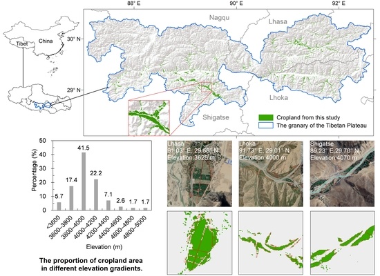
2.1. Study Area
2.2. Data
2.2.1. Landsat Data and Pre-Processing
2.2.2. Ground Truth Data
2.2.3. Other Data
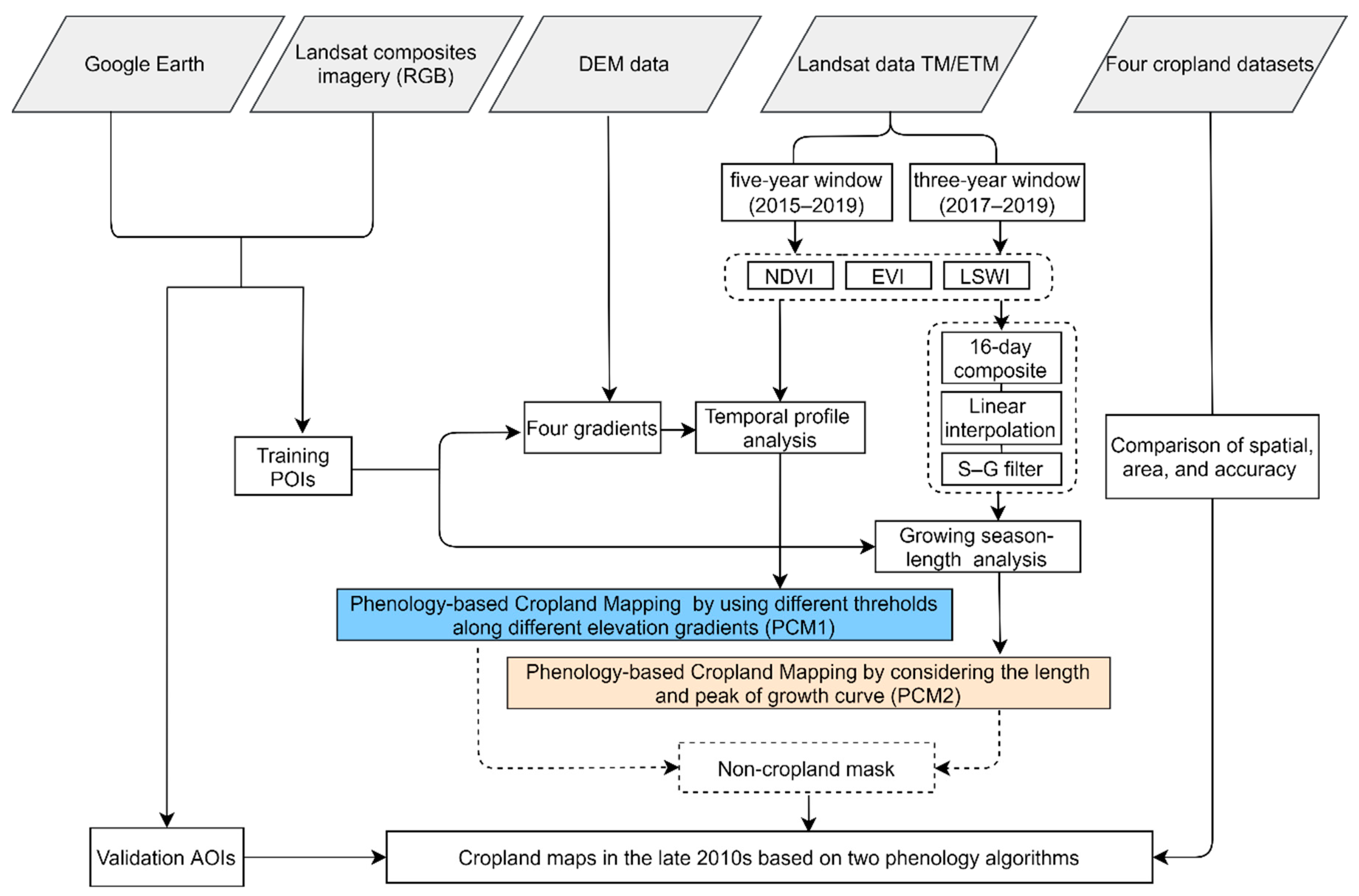
2.3. Methods
2.3.1. The First Phenology-Based Cropland Mapping (PCM1)
2.3.2. The Second Phenology-Based Cropland Mapping (PCM2)
2.3.3. Accuracy Assessment of Cropland Maps and Comparison with Existing Maps
3. Results
3.1. Accuracy Assessment
3.2. Cropland Map of BRTT in 2017–2019
3.3. Comparison of Penology-Based Map with Other Four Cropland Datasets
4. Discussion
4.1. Phenology-Based Approaches for Mapping Croplands in the Mountainous Area
4.2. Uncertainty and Implications
5. Conclusions
Supplementary Materials
Author Contributions
Funding
Data Availability Statement
Conflicts of Interest
References
- Zhang, G.; Dong, J.; Zhou, C.; Xu, X.; Wang, M.; Ouyang, H.; Xiao, X. Increasing cropping intensity in response to climate warming in Tibetan Plateau, China. Field Crop. Res. 2013, 142, 36–46. [Google Scholar] [CrossRef]
- Gong, J.; Li, J.; Yang, J.; Li, S.; Tang, W. Land Use and Land Cover Change in the Qinghai Lake Region of the Tibetan Plateau and Its Impact on Ecosystem Services. Int. J. Environ. Res. Public Health 2017, 14, 818. [Google Scholar] [CrossRef] [PubMed]
- Bai, W.; Yao, L.; Zhang, Y.; Wang, C. Spatial-temporal Dynamics of Cultivated Land in Recent 35 Years in the Lhasa River Basin of Tibet. J. Nat. Resour. 2014, 29, 623–632. [Google Scholar]
- Liu, X.D.; Chen, B.D. Climatic warming in the Tibetan Plateau during recent decades. Int. J. Climatol. 2000, 20, 1729–1742. [Google Scholar] [CrossRef]
- Cui, X.; Graf, H.-F.; Langmann, B.; Chen, W.; Huang, R. Climate impacts of anthropogenic land use changes on the Tibetan Plateau. Glob. Planet. Chang. 2006, 54, 33–56. [Google Scholar] [CrossRef] [Green Version]
- Li, S.; Yang, P.; Gao, S.; Chen, H.; Yao, F. Dynamic Changes and Developmental Trends of the Land Desertification in Tibetan Plateau over the Past 10 Years. Adv. Earth Sci. 2004, 19, 63–70. [Google Scholar]
- Zhao, Y.-Z.; Zou, X.-Y.; Cheng, H.; Jia, H.-K.; Wu, Y.-Q.; Wang, G.-Y.; Zhang, C.-L.; Gao, S.-Y. Assessing the ecological security of the Tibetan plateau: Methodology and a case study for Lhaze County. J. Environ. Manag. 2006, 80, 120–131. [Google Scholar] [CrossRef] [PubMed]
- Wang, X.; He, K.; Dong, Z. Effects of climate change and human activities on runoff in the Beichuan River Basin in the northeastern Tibetan Plateau, China. Catena 2019, 176, 81–93. [Google Scholar] [CrossRef]
- Galford, G.L.; Mustard, J.F.; Melillo, J.; Gendrin, A.; Cerri, C.C. Wavelet analysis of MODIS time series to detect expansion and intensification of row-crop agriculture in Brazil. Remote Sens. Environ. 2008, 112, 576–587. [Google Scholar] [CrossRef]
- Lu, M.; Wu, W.; Zhang, L.; Liao, A.; Peng, S.; Tang, H. A comparative analysis of five global cropland datasets in China. Sci. China Earth Sci. 2016, 59, 2307–2317. [Google Scholar] [CrossRef]
- Zhou, Y.; Dong, J.; Liu, J.; Metternicht, G.; Shen, W.; You, N.; Zhao, G.; Xiao, X. Are There Sufficient Landsat Observations for Retrospective and Continuous Monitoring of Land Cover Changes in China? Remote Sens. 2019, 11, 1808. [Google Scholar] [CrossRef] [Green Version]
- Zhang, M.; Chen, F.; Tian, B.; Liang, D.; Yang, A. High-Frequency Glacial Lake Mapping Using Time Series of Sentinel-1A/1B SAR Imagery: An Assessment for the Southeastern Tibetan Plateau. Int. J. Environ. Res. Public Health 2020, 17, 1072. [Google Scholar] [CrossRef] [PubMed] [Green Version]
- Ma, Q.; You, Q.; Ma, Y.; Cao, Y.; Zhang, J.; Niu, M.; Zhang, Y. Changes in cloud amount over the Tibetan Plateau and impacts of large-scale circulation. Atmospheric Res. 2021, 249. [Google Scholar] [CrossRef]
- Wang, X.; Zheng, D.; Shen, Y. Land use change and its driving forces on the Tibetan Plateau during 1990–2000. Catena 2008, 72, 56–66. [Google Scholar] [CrossRef]
- Li, S.; Zhang, Y.; He, F. Reconstruction of cropland distribution in Qinghai and Tibet for the past one hundred years and its spatiotemporal changes. Prog. Geogr. 2015, 34, 197–206. [Google Scholar]
- Li, S.; Wang, Z.; Zhang, Y. Crop cover reconstruction and its effects on sediment retention in the Tibetan Plateau for 1900–2000. J. Geogr. Sci. 2017, 27, 786–800. [Google Scholar] [CrossRef]
- Luo, J.; Chen, Q.; Liu, F.; Zhang, Y.; Zhou, Q. Methods for reconstructing historical cropland spatial distribution of the Yellow River-Huangshui River valley in Tibetan Plateau. Prog. Geogr. 2015, 34, 207–216. [Google Scholar]
- Jia, K.; Liang, S.; Wei, X.; Yao, Y.; Su, Y.; Jiang, B.; Wang, X. Land Cover Classification of Landsat Data with Phenological Features Extracted from Time Series MODIS NDVI Data. Remote Sens. 2014, 6, 11518–11532. [Google Scholar] [CrossRef] [Green Version]
- Dan, L. Study on Spatio-Temporal Variations of Crop Planting Areas in the Valley of Brahmaputra and Lhasa River and Nian-Chu River, Tibet, China. Master’s Thesis, Southwest University, Chongqing, China, 2017. [Google Scholar]
- Chu, D.; Shrestha, B.; Wang, W.; Zhang, Y.; Liu, L.; Pradhan, S. Land Cover Mapping in the Tibet Plateau Using MODIS Imagery. Resour. Sci. 2010, 32, 2152–2159. [Google Scholar]
- Leroux, L.; Jolivot, A.; Bégué, A.; Seen, D.L.; Zoungrana, B. How Reliable is the MODIS Land Cover Product for Crop Mapping Sub-Saharan Agricultural Landscapes? Remote Sens. 2014, 6, 8541–8564. [Google Scholar] [CrossRef] [Green Version]
- Wulder, M.A.; Masek, J.G.; Cohen, W.B.; Loveland, T.R.; Woodcock, C.E. Opening the archive: How free data has enabled the science and monitoring promise of Landsat. Remote Sens. Environ. 2012, 122, 2–10. [Google Scholar] [CrossRef]
- Roy, D.P.; Wulder, M.; Loveland, T.R.; Woodcock, C.; Allen, R.; Anderson, M.; Helder, D.; Irons, J.; Johnson, D.; Kennedy, R.; et al. Landsat-8: Science and product vision for terrestrial global change research. Remote Sens. Environ. 2014, 145, 154–172. [Google Scholar] [CrossRef] [Green Version]
- Zhong, L.; Gong, P.; Biging, G.S. Efficient corn and soybean mapping with temporal extendability: A multi-year experiment using Landsat imagery. Remote Sens. Environ. 2014, 140, 1–13. [Google Scholar] [CrossRef]
- Dong, J.; Xiao, X.; Menarguez, M.A.; Zhang, G.; Qin, Y.; Thau, D.; Biradar, C.; Moore, B. Mapping paddy rice planting area in northeastern Asia with Landsat 8 images, phenology-based algorithm and Google Earth Engine. Remote Sens. Environ. 2016, 185, 142–154. [Google Scholar] [CrossRef] [PubMed] [Green Version]
- Gao, F.; Anderson, M.C.; Zhang, X.; Yang, Z.; Alfieri, J.G.; Kustas, W.P.; Mueller, R.; Johnson, D.M.; Prueger, J.H. Toward mapping crop progress at field scales through fusion of Landsat and MODIS imagery. Remote Sens. Environ. 2017, 188, 9–25. [Google Scholar] [CrossRef] [Green Version]
- Wang, J.; Xiao, X.; Liu, L.; Wu, X.; Qin, Y.; Steiner, J.L.; Dong, J. Mapping sugarcane plantation dynamics in Guangxi, China, by time series Sentinel-1, Sentinel-2 and Landsat images. Remote Sens. Environ. 2020, 247, 16. [Google Scholar] [CrossRef]
- Xiao, X.; Boles, S.; Frolking, S.; Li, C.; Babu, J.Y.; Salas, W.; Moore, B. Mapping paddy rice agriculture in South and Southeast Asia using multi-temporal MODIS images. Remote Sens. Environ. 2006, 100, 95–113. [Google Scholar] [CrossRef]
- Griffiths, P.; Nendel, C.; Hostert, P. Intra-annual reflectance composites from Sentinel-2 and Landsat for national-scale crop and land cover mapping. Remote Sens. Environ. 2019, 220, 135–151. [Google Scholar] [CrossRef]
- Song, X.-P.; Potapov, P.V.; Krylov, A.; King, L.; Di Bella, C.M.; Hudson, A.; Khan, A.; Adusei, B.; Stehman, S.V.; Hansen, M.C. National-scale soybean mapping and area estimation in the United States using medium resolution satellite imagery and field survey. Remote Sens. Environ. 2017, 190, 383–395. [Google Scholar] [CrossRef]
- Ding, M.; Chen, Q.; Xin, L.; Li, L.; Li, X. Spatial and temporal variations of multiple cropping index in China based on SPOT-NDVI during 1999-2013. Acta Geogr. Sinica 2015, 70, 1080–1090. [Google Scholar]
- Zhang, G.L. Response and Adaption of Agro-Ecosystem to Climate Warming in the Region Of Brahmaputra River and Its Two Tributaries in Tibet. Ph.D. Thesis, Institute of Geographic Sciences and Natural Resources Research, Chinese Academy of Sciences, Beijing, China, 2011. [Google Scholar]
- Cheng, M.; Jin, J.; Zhang, J.; Jiang, H.; Wang, R. Effect of climate change on vegetation phenology of different land-cover types on the Tibetan Plateau. Int. J. Remote Sens. 2018, 39, 470–487. [Google Scholar] [CrossRef]
- Diao, C.; Wang, L. Incorporating plant phenological trajectory in exotic saltcedar detection with monthly time series of Landsat imagery. Remote Sens. Environ. 2016, 182, 60–71. [Google Scholar] [CrossRef]
- Wang, J.; Xiao, X.; Qin, Y.; Dong, J.; Geissler, G.; Zhang, G.; Cejda, N.; Alikhani, B.; Doughty, R.B. Mapping the dynamics of eastern redcedar encroachment into grasslands during 1984–2010 through PALSAR and time series Landsat images. Remote Sens. Environ. 2017, 190, 233–246. [Google Scholar] [CrossRef] [Green Version]
- Zhang, G.; Biradar, C.; Xiao, X.; Dong, J.; Zhou, Y.; Qin, Y.; Zhang, Y.; Liu, F.; Ding, M.; Thomas, R.J. Exacerbated grassland degradation and desertification in Central Asia during 2000–2014. Ecol. Appl. 2018, 28, 442–456. [Google Scholar] [CrossRef] [Green Version]
- Zhang, G.; Xiao, X.; Dong, J.; Kou, W.; Jin, C.; Qin, Y.; Zhou, Y.; Wang, J.; Menarguez, M.A.; Biradar, C. Mapping paddy rice planting areas through time series analysis of MODIS land surface temperature and vegetation index data. ISPRS J. Photogramm. Remote Sens. 2015, 106, 157–171. [Google Scholar] [CrossRef] [Green Version]
- Piao, S.; Friedlingstein, P.; Ciais, P.; Viovy, N.; Demarty, J. Growing season extension and its impact on terrestrial carbon cycle in the Northern Hemisphere over the past 2 decades. Glob. Biogeochem. Cycles 2007, 21, 11. [Google Scholar] [CrossRef]
- Dong, J.; Xiao, X.; Kou, W.; Qin, Y.; Zhang, G.; Li, L.; Jin, C.; Zhou, Y.; Wang, J.; Biradar, C.; et al. Tracking the dynamics of paddy rice planting area in 1986–2010 through time series Landsat images and phenology-based algorithms. Remote Sens. Environ. 2015, 160, 99–113. [Google Scholar] [CrossRef]
- Griffiths, P.; Kuemmerle, T.; Baumann, M.; Radeloff, V.C.; Abrudan, I.V.; Lieskovsky, J.; Munteanu, C.; Ostapowicz, K.; Hostert, P. Forest disturbances, forest recovery, and changes in forest types across the Carpathian ecoregion from 1985 to 2010 based on Landsat image composites. Remote Sens. Environ. 2014, 151, 72–88. [Google Scholar] [CrossRef]
- Paltridge, N.; Tao, J.; Unkovich, M.; Bonamano, A.; Gason, A.; Grover, S.; Wilkins, J.; Tashi, N.; Coventry, D. Agriculture in central Tibet: An assessment of climate, farming systems, and strategies to boost production. Crop. Pasture Sci. 2009, 60, 627–639. [Google Scholar] [CrossRef]
- Anders, A.M.; Roe, G.H.; Hallet, B.; Montgomery, D.R.; Finnegan, N.J.; Putkonen, J. Spatial patterns of precipitation and topography in the Himalaya. In Tectonics, Climate, and Landscape Evolution; Geological Society of America: Boulder, CO, USA, 2006; Volume 398, pp. 39–53. [Google Scholar]
- Tashi, N.; Yanhua, L.; Partap, T. Making Tibet Food Secure: Assessment of Scenarios; International Centre for Integrated Mountain Development: Kathmandu, Nepal, 2002; p. 171. [Google Scholar]
- Wei, X.; Yang, P.; Dong, G. Agricultural Development and Farmland Desertification in Middle “One River and Its Two Branches” River Basin of Tibet. J. Desert Res. 2004, 24, 196–200. [Google Scholar]
- Ping, L.I.; Gaihe, Y.; Yongzhong, F. Analysis of the structure of compound agriculture-herding ecological system in the YLN Region of Tibet. Agric. Res. Arid Areas 2007, 25, 180–184. [Google Scholar]
- Roy, D.; Kovalskyy, V.; Zhang, H.; Vermote, E.; Yan, L.; Kumar, S.; Egorov, A. Characterization of Landsat-7 to Landsat-8 reflective wavelength and normalized difference vegetation index continuity. Remote Sens. Environ. 2016, 185, 57–70. [Google Scholar] [CrossRef] [Green Version]
- Zhu, Z.; Wang, S.; Woodcock, C.E. Improvement and expansion of the Fmask algorithm: Cloud, cloud shadow, and snow detection for Landsats 4–7, 8, and Sentinel 2 images. Remote Sens. Environ. 2015, 159, 269–277. [Google Scholar] [CrossRef]
- Zhu, Z.; Woodcock, C.E. Object-based cloud and cloud shadow detection in Landsat imagery. Remote Sens. Environ. 2012, 118, 83–94. [Google Scholar] [CrossRef]
- Tucker, C.J. Red and photographic infrared linear combinations for monitoring vegetation. Remote Sens. Environ. 1979, 8, 127–150. [Google Scholar] [CrossRef] [Green Version]
- Huete, A.; Didan, K.; Miura, T.; Rodriguez, E.P.; Gao, X.; Ferreira, L.G. Overview of the radiometric and biophysical performance of the MODIS vegetation indices. Remote Sens. Environ. 2002, 83, 195–213. [Google Scholar] [CrossRef]
- Xiao, X.; Boles, S.; Liu, J.; Zhuang, D.; Frolking, S.; Li, C.; Salas, W.; Moore, B. Mapping paddy rice agriculture in southern China using multi-temporal MODIS images. Remote Sens. Environ. 2005, 95, 480–492. [Google Scholar] [CrossRef]
- Xiao, X.; Hagen, S.; Zhang, Q.; Keller, M.; Moore, B. Detecting leaf phenology of seasonally moist tropical forests in South America with multi-temporal MODIS images. Remote Sens. Environ. 2006, 103, 465–473. [Google Scholar] [CrossRef]
- Kandasamy, S.; Baret, F.; Verger, A.; Neveux, P.; Weiss, M. A comparison of methods for smoothing and gap filling time series of remote sensing observations—Application to MODIS LAI products. Biogeosciences 2013, 10, 4055–4071. [Google Scholar] [CrossRef] [Green Version]
- Ma, X.; Chen, S.; Deng, J.; Feng, Q.; Huang, X. Vegetation phenology dynamics and its response to climate change on the Tibetan Plateau. Acta Pratacult. Sin. 2016, 25, 13–21. [Google Scholar]
- Lehner, B.; Verdin, K.; Jarvis, A. New Global Hydrography Derived From Spaceborne Elevation Data. Eos Trans. Am. Geophys. Union 2008, 89, 93–94. [Google Scholar] [CrossRef]
- Liu, J.; Kuang, W.; Zhang, Z.; Xu, X.; Qin, Y.; Ning, J.; Zhou, W.; Zhang, S.; Li, R.; Yan, C.; et al. Spatiotemporal characteristics, patterns, and causes of land-use changes in China since the late 1980s. J. Geogr. Sci. 2014, 24, 195–210. [Google Scholar] [CrossRef]
- Chen, J.; Chen, J.; Liao, A.P.; Cao, X.; Chen, L.J.; Chen, X.H.; He, C.Y.; Han, G.; Peng, S.; Lu, M.; et al. Global land cover mapping at 30m resolution: A POK-based operational approach. ISPRS J. Photogramm. Remote Sens. 2015, 103, 7–27. [Google Scholar] [CrossRef] [Green Version]
- Yu, L.; Wang, J.; Gong, P. Improving 30 m global land-cover map FROM-GLC with time series MODIS and auxiliary data sets: A segmentation-based approach. Int. J. Remote Sens. 2013, 34, 5851–5867. [Google Scholar] [CrossRef]
- Sulla-Menashe, D.; Gray, J.; Abercrombie, S.P.; Friedl, M.A. Hierarchical mapping of annual global land cover 2001 to present: The MODIS Collection 6 Land Cover product. Remote Sens. Environ. 2019, 222, 183–194. [Google Scholar] [CrossRef]
- Xue-Yong, Z.; Sen, L.; Chun-Lai, Z.; Guang-Rong, D.; Yu-Xiang, D.; Ping, Y. Desertification and control plan in the Tibet Autonomous Region of China. J. Arid. Environ. 2002, 51, 183–198. [Google Scholar] [CrossRef]
- Olofsson, P.; Foody, G.; Herold, M.; Stehman, S.V.; Woodcock, C.E.; Wulder, M.A. Good practices for estimating area and assessing accuracy of land change. Remote Sens. Environ. 2014, 148, 42–57. [Google Scholar] [CrossRef]
- Chicco, D.; Jurman, G. The advantages of the Matthews correlation coefficient (MCC) over F1 score and accuracy in binary classification evaluation. BMC Genom. 2020, 21, 13. [Google Scholar] [CrossRef] [Green Version]
- Olofsson, P.; Foody, G.; Stehman, S.V.; Woodcock, C.E. Making better use of accuracy data in land change studies: Estimating accuracy and area and quantifying uncertainty using stratified estimation. Remote Sens. Environ. 2013, 129, 122–131. [Google Scholar] [CrossRef]
- Zhang, R.; Ouyang, Z.-T.; Xie, X.; Guo, H.-Q.; Tan, D.-Y.; Xiao, X.-M.; Qi, J.-G.; Zhao, B. Impact of Climate Change on Vegetation Growth in Arid Northwest of China from 1982 to 2011. Remote Sens. 2016, 8, 364. [Google Scholar] [CrossRef] [Green Version]
- Chandrasekar, K.; Sai, M.V.R.S.; Roy, P.S.; Dwevedi, R.S. Land Surface Water Index (LSWI) response to rainfall and NDVI using the MODIS Vegetation Index product. Int. J. Remote Sens. 2010, 31, 3987–4005. [Google Scholar] [CrossRef]
- Gao, F.; Masek, J.; Schwaller, M.; Hall, F. On the blending of the Landsat and MODIS surface reflectance: Predicting daily Landsat surface reflectance. IEEE Trans. Geosci. Remote Sens. 2006, 44, 2207–2218. [Google Scholar] [CrossRef]
- Niu, Z.; Wu, M.; Wang, C. Use of MODIS and Landsat time series data to generate high-resolution temporal synthetic Landsat data using a spatial and temporal reflectance fusion model. J. Appl. Remote Sens. 2012, 6, 13. [Google Scholar] [CrossRef]
- Knauer, K.; Gessner, U.; Fensholt, R.; Forkuor, G.; Kuenzer, C. Monitoring Agricultural Expansion in Burkina Faso over 14 Years with 30 m Resolution Time Series: The Role of Population Growth and Implications for the Environment. Remote Sens. 2017, 9, 132. [Google Scholar] [CrossRef] [Green Version]
- Gao, F.; Hilker, T.; Zhu, X.; Anderson, M.; Masek, J.; Wang, P.; Yang, Y. Fusing Landsat and MODIS Data for Vegetation Monitoring. IEEE Geosci. Remote Sens. Mag. 2015, 3, 47–60. [Google Scholar] [CrossRef]
- Gong, P.; Wang, J.; Yu, L.; Zhao, Y.; Zhao, Y.; Liang, L.; Niu, Z.; Huang, X.; Fu, H.; Liu, S.; et al. Finer resolution observation and monitoring of global land cover: First mapping results with Landsat TM and ETM+ data. Int. J. Remote Sens. 2013, 34, 2607–2654. [Google Scholar] [CrossRef] [Green Version]
- Ding, M.; Zhang, Y.; Sun, X.; Liu, L.; Wang, Z.; Bai, W. Spatiotemporal variation in alpine grassland phenology in the Qinghai-Tibetan Plateau from 1999 to 2009. Chin. Sci. Bull. 2013, 58, 396–405. [Google Scholar] [CrossRef] [Green Version]
- Waldner, F.; Schucknecht, A.; Lesiv, M.; Gallego, J.; See, L.; Pérez-Hoyos, A.; D’Andrimont, R.; de Maet, T.; Bayas, J.C.L.; Fritz, S.; et al. Conflation of expert and crowd reference data to validate global binary thematic maps. Remote Sens. Environ. 2019, 221, 235–246. [Google Scholar] [CrossRef]
- Peña-Barragán, J.M.; Ngugi, M.K.; Plant, R.E.; Six, J. Object-based crop identification using multiple vegetation indices, textural features and crop phenology. Remote Sens. Environ. 2011, 115, 1301–1316. [Google Scholar] [CrossRef]
- Yin, H.; Prishchepov, A.V.; Kuemmerle, T.; Bleyhl, B.; Buchner, J.; Radeloff, V.C. Mapping agricultural land abandonment from spatial and temporal segmentation of Landsat time series. Remote Sens. Environ. 2018, 210, 12–24. [Google Scholar] [CrossRef]


| Product | Satellite Sensor | Spatial Resolution (m) | Periods | Class |
|---|---|---|---|---|
| CLUDs | Landsat TM/ETM+ | 100 | 2015 | 25 |
| GlobeLand30 | Landsat/TM, HJ/CCD | 30 | 2020 | 10 |
| FROM-GLC | Landsat TM | 30 | 2017 | 10 |
| MCD12Q1 | Terra/Aqua | 500 | 2019 | 17 |
| Methods | Class | PA | Adjusted PA | UA | Adjusted UA | OA | Adjusted OA | Area | Estimated Area |
|---|---|---|---|---|---|---|---|---|---|
| (%) | (km2) | ||||||||
| PCM1 | Cropland | 85.4 | 62.2 | 92.6 | 92.6 | 98.0 | 98.4 | 1724 | 2565 ± 94 |
| Noncropland | 99.3 | 99.8 | 97.4 | 98.5 | |||||
| PCM2 | Cropland | 92.5 | 81.8 | 90.8 | 90.8 | 98.8 | 99.2 | 1782 | 1979 ± 52 |
| Noncropland | 99.3 | 99.7 | 99.4 | 99.4 | |||||
| PCM2 | CLUDs | GlobeLand 30 | FROM-GLC | MCD12Q1 | |
|---|---|---|---|---|---|
| Adjusted OA (%) | 98.8 | 98.8 | 97.4 | 95.1 | 94.5 |
| MCC | 0.911 | 0.898 | 0.798 | 0.505 | 0.413 |
| Adjusted Commission error (%) | 9.2 | 5.1 | 20.1 | 2.3 | 7.1 |
| Adjusted Omission error (%) | 18.2 | 20.6 | 28.3 | 86.6 | 85.9 |
Publisher’s Note: MDPI stays neutral with regard to jurisdictional claims in published maps and institutional affiliations. |
© 2021 by the authors. Licensee MDPI, Basel, Switzerland. This article is an open access article distributed under the terms and conditions of the Creative Commons Attribution (CC BY) license (https://creativecommons.org/licenses/by/4.0/).
Share and Cite
Di, Y.; Zhang, G.; You, N.; Yang, T.; Zhang, Q.; Liu, R.; Doughty, R.B.; Zhang, Y. Mapping Croplands in the Granary of the Tibetan Plateau Using All Available Landsat Imagery, A Phenology-Based Approach, and Google Earth Engine. Remote Sens. 2021, 13, 2289. https://doi.org/10.3390/rs13122289
Di Y, Zhang G, You N, Yang T, Zhang Q, Liu R, Doughty RB, Zhang Y. Mapping Croplands in the Granary of the Tibetan Plateau Using All Available Landsat Imagery, A Phenology-Based Approach, and Google Earth Engine. Remote Sensing. 2021; 13(12):2289. https://doi.org/10.3390/rs13122289
Chicago/Turabian StyleDi, Yuanyuan, Geli Zhang, Nanshan You, Tong Yang, Qiang Zhang, Ruoqi Liu, Russell B. Doughty, and Yangjian Zhang. 2021. "Mapping Croplands in the Granary of the Tibetan Plateau Using All Available Landsat Imagery, A Phenology-Based Approach, and Google Earth Engine" Remote Sensing 13, no. 12: 2289. https://doi.org/10.3390/rs13122289
APA StyleDi, Y., Zhang, G., You, N., Yang, T., Zhang, Q., Liu, R., Doughty, R. B., & Zhang, Y. (2021). Mapping Croplands in the Granary of the Tibetan Plateau Using All Available Landsat Imagery, A Phenology-Based Approach, and Google Earth Engine. Remote Sensing, 13(12), 2289. https://doi.org/10.3390/rs13122289