An Analysis of Bare Soil Occurrence in Arable Croplands for Remote Sensing Topsoil Applications

Abstract

A better comprehension of soil properties and processes permits a progress in agricultural management effectiveness, together with a diminution of environmental damage and more beneficial use of resources. This research investigated the usage of multispectral (Sentinel-2 MSI) satellite data at the farm/regional level, for the identification of agronomic bare soil presence, utilizing bands of the spectral range from visible to shortwave infrared. The research purpose was to assess the frequency of cloud-free bare soil time-series images available during the year in typical agricultural areas, needed for the development of digital soil mapping (DSM) approaches for agricultural applications, using hyperspectral satellite missions such as current PRISMA and the planned EnMAP or CHIME. The research exploited the Google Earth Engine platform, by processing all available cloud-free Sentinel-2 images throughout a time span of four years. Two main results were obtained: (i) bare soil frequency, indicating where and when a pixel (or an agricultural field) was detected as bare surface in three representative agricultural areas of Italy, and (ii) a temporal sensitivity analysis, providing the acquisition frequency of useful bare soil images applicable for the retrieval of soil variables of interest. It was shown that, in order to provide for an effective agricultural soil monitoring capability, a revisit frequency in the range of five to seven days is required, which is less than the planned specifications e.g., of PRISMA or CHIME hyperspectral missions, but could be addressed by combining data from the two sensors.

1. Introduction

Soil is a highly dynamic and vulnerable ecosystem, and preserving its quality is essential for sustainable agriculture production and viable food security [1,2]. However, anthropic activities such as agricultural practices [3] and urbanizations [4] and poor soil management have caused degradation of soil structure, erosion, poor chemical and physical properties [1,3], and thus, reduced the arable soil areas. Holistic management of many agro-engineering activities such as irrigation and crop monitoring [5], fertilizer application [6], and land use planning [7] depends on the explicit spatial information of soil properties and variability. These reasons motivate an increasing necessity of affordable, consistent, large-scale, full exposure soil data [2].

From the first world soil map in 1981 by the Food and Agriculture Organization (FAO), researches have been employing different methodology to develop soil maps on a coarse spatial resolution on a global scale (e.g., the Harmonized World Soil Database [8], the European Soil Database [9]) or finer resolution in nationwide or regional surveys (e.g., the American Web Soil Survey [10] and the Soil Survey Geographic Data Base [11]). Nevertheless, the spatial resolution of existing soil maps, even of on-going global or continental digital soil mapping efforts such as SoilGrids [12], can be of insufficient detail to expose local-scale soil variability and lack temporal resolution due to the expense and labor required to update the underlying information layers [13].

Achieving higher comprehension of soil, its characteristics, processes, and functions, require an advancement of the effective methodologies to quantify and surveil it at diverse spatial and temporal levels. Traditional laboratory techniques used to analyze soil properties are mostly impracticable in this context, being time-consuming and costly [14].

Remote sensing is nowadays a well-developed discipline that has been largely used for developing several crop-dependent datasets (e.g., [15,16]) and improving spatiotemporal variability of the remotely sensed datasets using fusion techniques (e.g., [17,18]). Given these potentials in using the space-based Earth Observation (EO), similar frameworks could be adapted and combined with available soil mapping methods to increase the temporal and spatial resolution of soil data in a cost-effective way and a global coverage [2]. Nevertheless, satellite EO information, along with ground-based measurements and modelling have been marginally used in an operational way by national and international entities in charge of mapping, surveying and reporting on soils. With the advance of operating EO systems, e.g., Copernicus, the free and open-access earth observation data policy as well as cloud-based access and processing (e.g., DIAS), an earth observation-based Soil surveying System becomes feasible nowadays [19]. This is made even more possible by the forthcoming availability of high signal-to-noise ratio space-borne imagery spectrometers in addition to PRISMA, such as EnMAP [20], HISUI [21], SHALOM [22], NASA-SBG (Surface Biology and Geology), HySpex2 [23] and the Sentinel-10/CHIME (Copernicus Hyperspectral Imaging Mission for the Environment) [24].

The use of optical sensors for agricultural soil monitoring and mapping, however, relies on the availability of exposed bare soil, preferably at seedbed conditions, to minimize the influence of confounding factors such as vegetation residues and soil roughness. The accessible bare soil areas, needed for the mapping of the soil properties from remote sensing, changes depending on the acquisition dates because of crop rotations. Besides, in the available bare soil scenes, topsoil state changes, principally regarding soil humidity and roughness following tillage processes [25].

Over the years, novel methodologies related to bare soil exposure detection have been proposed, progressing into multi-temporal methodologies for higher coverage of bare topsoil [13,26,27,28,29,30]. In agricultural areas, with crop rotations or bare/ vegetated states alternation, multi-temporal images present a solution to increase the surface of detected bare soil [31,32,33]. Diek et al. [33] suggested a multi-temporal composite imagery method delivered from the Airborne Prism Experiment (APEX) for soil surveying. The authors merged three airborne images from similar plots at different collection dates, doubled the number of bare soil pixels, and enhanced the spatial representation of the soil area. Demattê et al. [29,34] established a methodology for detecting contiguous surfaces of soil exposure by fusing numerous scenes collected at precise dates of the agricultural season when soil exposure was relevant. The mentioned strategy is based on a linear spectral mixture model to distinguish between soils and vegetation [27], followed by a series of image-processing steps using NDVI and band combinations to specify the real nature of the pixel. In their research, the surface’ bare soil coverage increased from 36% (one image) to 75% (for the fused image) and allowed the mapping of the surface soil texture. Diek et al. [26] achieved a 90% coverage for the Swiss Plateau (Switzerland) from five years of Landsat images and the Barest Soil Composite methodology. Rogge et al. [13] modelled the Soil Composite Mapping Processor (SCMaP) as a strategy to overcome restricted soil exposure and map soil properties in Germany.

In this research, we hypothesize that monthly-basis agricultural bare soil occurrence is effective for topsoil applications and a moderate satellite revisit frequency (less than or at the range of five to seven days) is required for soil studies. To verify this hypothesis, we carried out a temporal sensitivity analysis. All available Sentinel-2 scenes between 2016 and 2019 were utilized, from the Google Earth Engine (GEE) platform, to maximize the bare soil cover across a large farming region. To demonstrate the functionality of the work, we present a case study for Italy. We obtained the exposed bare soil frequency maps for some typical agricultural areas of the Northern, Central and Southern Italy from the bare soil index. The research provides three primary product levels which comprise: (i) the temporal distribution of bare agricultural soils; (ii) a statistical evaluation of the temporal occurrence of bare soils; and, (iii) temporal sensitivity analysis of cloud-free bare soil image frequency.

2. Materials and Methods

In this research, a novel strategy was developed to use per-pixel bare soil surface exposure detection. The approach is based on multiple Sentinel-2 scenes to design a frequency map of exposed soils. The method presented here differs from the references mentioned above for several points. Primarily, the main objective of the mentioned references [13,26,35] was to develop exposed soil composites, i.e., a static product, whereas we were more interested in assessing the seasonal occurrence of bare soil frequency in arable croplands, thus investigating the dynamic and temporal aspect rather more. Secondly, temporal sensitivity analysis can be used to guide bare soil image acquisitions with hyperspectral sensors. The higher revisit time provided helps to detect changes in soil variability and increase the number of pixels with bare soil, which can influence the spatial predictions of soil properties. The evaluation of revisit time (temporal sensitivity analysis) forms a critical component of the soil studies. Thirdly, the dynamics of bare soil area reflectance could be examined by using multiple bare soil acquisition dates, rather than with a static bare soil composite. This could allow studying the soil surfaces dynamic changes across the years.

2.1. Study Area

Three study areas have been selected for the bare soil frequency demonstration in Italy, specifically in representative sites of variable intensive arable agricultural systems in Northern, Central, and Southern Italy (Figure 1).

The experimental field area representative of the North of Italy comprises the Province of Ferrara in the Po-plain, which is the most intensive agricultural area of Italy. The climate in the region is warm and temperate (Köppen–Geiger classification). The annual mean precipitation is 691 mm (late spring and autumn peaks), and the annual mean temperature is 13.6 °C. The soil textures are mainly clayey and silty. Based on the Italian Institute for Statistics (ISTAT), the overall agricultural area englobes the following crop classes: arable land, permanent tree orchards, and permanent pastures. The “arable land” class is the sum of cereals, legumes, tubers, fresh vegetables and industrial crops. Fruit plantations, vineyards and olive orchards characterize the “permanent tree crops” class. For each crop class, the category of arable land covers 93% of the total agricultural area, while trees and forages represent 7% and 1%, respectively. The principal crops grown in the area are winter wheat followed by maize, durum wheat, soybeans and lucerne. These crop categories designate two main crop growth seasons, i.e., from February to April for winter-spring crops, e.g., wheat and soybeans, and from June to August for summer crops, e.g., maize.

For the Centre of Italy, the area under investigation is the Province of Rome in the Lazio region. The climate of the area is categorized by mild springs and autumns, monthly maximum temperatures in summer (26.0–29.6 °C, June–August) and monthly minimum temperatures in winter (3.1–4.4 °C, December–February) (CRA-CMA, 1981–2010). The main soil characteristics variability are as follow: organic carbon density (299–606 [g/dm³]); soil organic carbon (28–107 [t/ha]); bulk density (83–142 [g/cm³]); clay content (125–521 [g/kg]); coarse fragments (49–319 [cm³/dm³]); cation exchange capacity at pH 7 (184–438 [mmol(C)/kg]); nitrogen (188–844 [cg/kg]); and soil organic carbon (234–1362 [dg/Kg]) [36]. The main soil classes according to the World Reference Base [37] are Fluvisols, Cambisols, Luvisols, Vertisols, and Acrisols. The main crops cultivated in this area are olives followed by lucerne, durum wheat and wine grapes. For each crop class, the category of arable land covers 45% of the total agricultural area, while trees and pastures represent 22% and 33%, respectively.

Capitanata is the investigated area in Southern Italy, with an area of 720,000 ha. It extends over the Province of Foggia, in the Apulia Region. The climate is “accentuated thermomediterranean” (Unesco-FAO classification), having temperature values below 0 °C (till −10 °C) in winter [38] and up to 40 °C in summer. Precipitation is unequally distributed over the year and is typically intense in the winter, with a long-term annual average of 550 mm. Generally, the soils are deep, clay/silty-clay, and Vertisol of alluvial origin. The area is an intensive cultivation area, predominantly cultivated with durum wheat. Capitanata is among the main areas in Italy in terms of the production of durum wheat and tomato, as well as for permanent crops as olives and grapes. For each crop category, the arable land class covers 64% of the total agricultural area, while trees and pastures represent each one 18%.

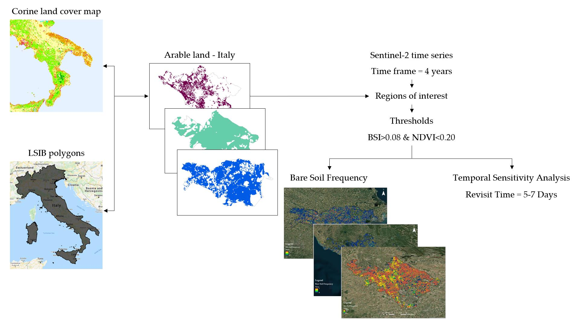
The delineation of the country and Province borders in the Google Erath Engine platform was done with the Large-Scale International Boundary (LSIB) Polygons of the United States Department of State (USDOS).

2.2. Methodology for Exposed Bare Soil Occurrence

The generating of the exposed bare soil frequency is illustrated in Figure 2, and hereafter, the steps followed are described. These include: (A) the satellite data pre-processing stages (Section 2.2.1); (B) the production of the exposed bare pixels maps (Section 2.2.2), (C) the explanation of the utilized bare soil indices (Section 2.2.3) and (D) the creation of the bare soil frequency maps, together with the definition of the thresholds (Section 2.2.4).

2.2.1. Pre-Processing of Satellite Data

For this study, all available Sentinel-2 imagery covering the three study sites were selected on the Google Earth Engine (GEE) platform, for the time interval from 1 January 2016 to 31 December 2019 (for a total of 2130). Sentinel-2 data used in this study included the 13 spectral bands of the MSI (443–2190 nm), with a swath width of 290 km and a pixel size of 10 m (four visible and near-infrared channels), 20 m (six red edge and shortwave infrared channels) and 60 m (three atmospheric correction channels). We selected only the bands in the visible (Vis), near- (NIR) and shortwave- (SWIR) infrared range (

Table 1. Selected Sentinel-2 satellite bands used in this study.

	Sentinel-2
	Wavelength (nm)	Resolution (m)	Band Number
Blue	490	10	2
Green	560	10	3
Red	665	10	4
NIR	842	10	8
SWIR1	1610	20	11

), even though Sentinel-2 sensors deliver other bands. These spectral ranges are recognized as efficient for soil characteristics studies [26,39]. Subsequently, the remaining spectral bands were excluded. Pre-processing included the exclusion of the cloudy images. A maximum of 45% cloud presence was set.

2.2.2. Exposed Bare Pixels Detection

The agricultural areas chosen for the current work were firstly classified into (I) arable land area and (II) non-arable land area. The arable area was outlined using the Corine Land Cover (CLC) 2012 map [40]. The basic technical parameters of CLC are 44 classes, 25 hectares minimum mapping unit (MMU), and 100 m minimum mapping width. The CLC classes include artificial surfaces, forest and semi-natural areas, wetlands, agricultural areas and water bodies. For our study we only selected the arable area including the classes non-irrigated arable land (land cover class value = 211) and permanently irrigated land (land cover class value = 212). The other classes of the Corine map were not considered.

2.2.3. Bare Soil Indices

Cropland can present zones of exposed soil for short time periods due to agricultural operations. These zones alternate from exposed soil to active vegetation areas, theoretically more than once every year. The methodology employed acknowledges this fact, developing a bare soil mask that is obtained by the use of a vegetation index (NDVI) that differentiates evidently green vegetation (high NDVI values) from dry vegetation or bare soil (low NDVI values).

Given that the areas covered by water, forests and urban areas were excluded from the study, the use of the minimum normalized difference vegetation index NDVI [41,42] presents either bare soil or crop residues. The NDVI was employed to the discriminate vegetation cover from bare soil areas and the combination of soil and dead vegetation [28,43]. The NDVI index uses the Red (band 4) and NIR (band 8) channels of Sentinel-2, which are valuable in efficiently distinguishing photosynthetic vegetation from other land covers. Fusing the NDVI index together with a bare soil index can provide a good way to further identify bare soil and was already attempted by numerous researchers [44,45,46,47].

$$\mathrm{NDVI}=\frac{\mathrm{NIR}-\mathrm{Red}}{\mathrm{NIR}+\mathrm{Red}}$$

(1)

NDVI does not present unique spectral information that can be employed to differentiate soils from all other land covers. Therefore, to overcome this limitation we also included a bare soil index (BSI) to extract exposed soil pixels. Rikimaru et al. [44] proposed the bare soil index (BSI [–]) (Equation (2)). The BSI is a combination of the NDVI and the Normalized Difference Built-up Index (NDBI) [47]. BSI is a spectral index that strengthens the detection of exposed soil surfaces and uncultivated areas [48] relying on soil characteristics. In this case we used the original BSI based on the SWIR1 reflectance:

$$\mathrm{BSI}=\frac{\left(\mathrm{SWIR}1+\mathrm{Red}\right)-\left(\mathrm{NIR}+\mathrm{Blue}\right)}{\left(\mathrm{SWIR}1+\mathrm{Red}\right)+\left(\mathrm{NIR}+\mathrm{Blue}\right)}$$

(2)

Values range between −1 and 1, where a high value designates the barest soil.

This index has been mostly employed in forest studies to separate between bare soil and other cover classes [49,50]. It was also employed to map and survey bare soil land [51,52]. Another benefit of the BSI is the separation of the vegetation cover from the rest of the background types (entirely bare, sparse canopy or dense canopy) [53,54]. Practice and prior acquaintance of the study area are critical for the definition of the optimal threshold values for identifying bare soil. Diek et al. [26] specified that the BSI performed significantly better than the minimum NDVI with regards to the discrimination of tree shadows, cloud shadows and low hanging clouds.

For all the studied agricultural area, the cloud-free BSI and NDVI values were calculated based on the months January to December to extract the exposed bare soil areas in the Sentinel-2 time series. Non-agricultural areas and other excluded pixels were not used in any further analysis.

The success of the methodology is the definition of relevant thresholds for bare soil discrimination. Different agricultural fields were chosen in the three study sectors to identify these thresholds, which should also be generally valid over the whole study region and over different study periods. Soils are likely to have relatively small NDVI values, around 0.1 to 0.2 [55]. We have identified a threshold of 0.20 for NDVI, and all pixels above this range were considered as non-bare soil.

The BSI threshold was calculated taking into consideration reference information. We delineated a number of agricultural fields of the Northern, Central, and Southern study areas in different parts of Italy (Ferrara (n = 5), Rome (n = 4), Capitanata (n = 4)) on the Sentinel-2 time series. The samples were selected on the basis of (i) the diversity of soil properties and texture, and (ii) having different vegetation responses. From inspection of the Sentinel-2 data, we classified the agricultural area into bare and non-bare soil, by setting a BSI threshold of 0.08. All pixels with BSI values above this threshold were classified as bare soil. This threshold was chosen as follow: we examined, over the agricultural years (2016–2019), the time series of the BSI for all the selected agricultural fields under each area. For each region (Ferrara, Rome and Capitanata), a time series chart was plotted separately. The threshold of 0.08 was chosen by considering the time trends over the three areas and the known crop rotations of the fields. To assess the accuracy of the classification performed using these criteria, we computed the error matrix, to determine the user’s and producer’s accuracy of the bare soil class, as described in Section 2.3.

2.2.4. Bare Soil Frequency

Regarding the exposed Bare Soil frequency, we considered only arable land agricultural areas. For this land use, we identified all pixels with a BSI and NDVI values, respectively, above and below the selected thresholds. The frequency of bare soil occurrence was estimated from the number of times a pixel was assigned to the bare soil class, divided by the total number of cloud-free images available in the same period.

From the monthly bare soil frequency maps of each year, we obtained the monthly average bare soil frequency maps over the four years. Furthermore, we calculated the percentage of pixels of bare soil frequency classes for the monthly-average over the four years falling into five classes (centered on 0%, 25%, 50%, 75%, 100%).

2.3. Validation

For the validation of the bare soil classification accuracy, we computed the user’s and producer’s accuracy of the exposed bare soil frequency, and the total accuracy. For this purpose, 500 points were randomly selected for each study area separately, and only in arable land agricultural soils (1500 points in total). These 500 random sample points were chosen through random classification by means of ArcGIS. Each sample point represents one pixel. Subsequently, these samples were compared with high-resolution scenes from Google Earth Pro.

During the validation process, we selected the Sentinel-2 images with acquisition dates close to Google Earth Pro images acquisitions. This was done to examine, for each of the 500 points, the correspondence between known ground cover data (ground truth) and the related results of the bare soil mapping. A common method for assessing classification accuracy is the formulation of a classification error matrix.

The overall accuracy was calculated by dividing the entire number of properly classified pixels by the entire number of reference pixels. The producer accuracy resulted from dividing the number of properly classified pixels in each class by the number of training set pixels used for that class. This shows how well pixels of a specified class in the training set are classified. The user’s accuracy was calculated by dividing the number of properly classified pixels in each class by the total number of pixels that were classified in that class. This is an assessment of the commission error and illustrates the probability that a pixel of a specified class truly represents that class on the ground.

2.4. Temporal Sensitivity Analysis

A temporal sensitivity analysis considering all the bare soil frequency maps for topsoil properties and mapping applications was carried out. Both cloud cover as well as the yearly occurrence of bare soil were considered during the temporal sensitivity analysis. The temporal sensitivity analysis, relative to the acquisition frequency of current or forthcoming satellite hyperspectral imagers, was performed on the three test areas of Ferrara, Rome and Capitanata.

Using a Google Earth Engine (GEE) script, we extracted the BSI and NDVI time series of Sentinel-2 images for the time interval starting from January 2016 to December 2019, for the agricultural arable lands of the three areas: Ferrara (five experimental plots), Rome (four experimental plots) and Capitanata (four experimental plots). A condition was set for the dates whose correspondent Bare Soil Index BSI (by pixel) is higher than 0.08 and Normalized Difference Vegetation Index NDVI is lower than 0.20. The periods for which this criterion was true were selected. For each two successive selected dates, the difference of days in between was calculated. Average per days per year, per area was computed.

Furthermore, we downloaded from the Nasa Earth Observations NEO [56], the monthly cloud fraction from January to December (2016, 2017, 2018, and 2019). The monthly data is retrieved from the product “Cloud fraction 1-month TERRA/MODIS data”.

For the selection of the best revisit time of the satellite, we calculated the total number of images that would be available for the research period considering the cloud fraction. The test was carried out hypothesizing five revisit times: 30 days, 15 days, 10 days, 7 days, and 5 days, using the equation:

$$\mathrm{N}.\mathrm{of}\mathrm{available}\mathrm{images}\mathrm{per}\mathrm{month}=\frac{\mathrm{N}.\mathrm{of}\mathrm{days}\mathrm{per}\mathrm{month}}{\mathrm{n}-\mathrm{days}}\ast \left(1-\mathrm{cloud}\mathrm{fraction}\right)$$

(3)

where n-days = 30, 15, 10, 7 or 5.

We then calculated the probability of cloud-free bare soil frequency occurrence, by multiplying the annual probability of bare soil frequency above 75% (calculated from the four year averages of the bare soil pixel fractions as described in Section 2.2.4), and the average number of the four years available cloud-free images expected as a function of satellite revisit time (RT) for the three areas.

3. Results and Discussion

In this section we present the results of the pre-processing of the Sentinel-2 images (Section 3.1); the production of the exposed bare pixels detection including the selected bare soil indices as well as the definition of the thresholds (Section 3.2); the validation of the exposed bare soil prediction on the basis of the selected bare soil thresholds (Section 3.3); and the results of the production of the Bare Soil Frequency (Section 3.4). Finally, we show the temporal sensitivity analysis (Section 3.5).

3.1. Cloud-Free Sentinel-2 Data Availability

Figure 3 shows the monthly number of cloud-free Sentinel-2 scenes existing for the three study sites. The availability of the satellite data shows fluctuations resulting from cloud cover presence, which is frequently the case in winter. Additionally, the number of available images changed over the years. The period of 2016 to 2017 could only rely on Sentinel 2A data, clearly providing a reduced dataset. The periods of 2017 to 2019 could exploit both Sentinel 2A and 2B data. The results presented, for some typical cropland areas of Italy, Sentinel-2 data offered detailed (10 m spatial resolution) soil data among 2016 and 2019.

The methodology adopted in this work, is based on the four-years’ time range to produce the different bare soil frequency maps. The four years’ period choice was based principally on supplying sufficient scenes to detect exposed bare soil pixels with high spatial resolution. Additionally, four years presented an adequate amount of data for statistical analysis. Nevertheless, the availability of images throughout the season can change among different regions of Italy, which may influence the number of times in which bare soil images would be available. In the four years considered, the number of cloud-free images available was higher for the Central Italy study area, with a mean annual value of 164, followed by the South of Italy with an annual mean of 82, whereas on average the number of images available for the North Italy study area was of 38.

The possible changes of surface soil conditions are also an important factor to take into account when selecting the time range. Since the pedology will be invariant, any variations in the topsoil during or across the four-years’ time interval will be brought about by other factors associated to (i) small scale change in humidity or farming practices (e.g., spreading of organic fertilizers, tillage); (ii) land cover/land use variations (e.g., grassland to cropland); or (iii) soil degradation and/or soil erosion caused by natural (e.g., flooding, long-term large scale climatic changes) or anthropogenic variations.

3.2. Thresholding of the Chosen Indices

Figure 4, Figure 5 and Figure 6 present (A) the BSI and (B) the NDVI for the pixels in the set of selected agricultural fields of the agricultural areas of Ferrara, Rome, and Capitanata, respectively. From Figure 4A, Figure 5A, and Figure 6A, the BSI time trend provides an indication on when agricultural fields are bare, how frequently and for what length of time. Ferrara agricultural area growing season is extended from October to July. The moment of maximum bare soil occurrence (August and September) is an indication of when crops were sown and harvested. It is possible to classify the crops on the area as relatively winter crops as they have a long growth season and an NDVI reaches a maximum in early summer. Rome and Capitanata agricultural areas are presenting the same results with a bare area time interval starting from July to September, which reveals a growth season starting in October and ending in June.

In croplands, the extraction of bare soil surfaces is not always well-defined. It could be, for example, fallow (unmanaged bare soil), or cultivated under crop rotation with various degrees of crop residues or sparse vegetation cover. According to the application, this could influence the results. In our case, we defined two thresholds 0.08 for the BSI and 0.20 for the NDVI. The bare soil frequency can be computed across any area and time interval with an adequate availability of Sentinel-2 scenes. On the basis of the hypothesis that the fluctuation between bare soil and vegetation reveals crop rotations, it is possible to differentiate between cropland and pasture within an agricultural region (i.e., a field is classified as cropland if it has at least one bare soil occurrence in the selected period). This is important for land resources modelling, especially in cases where these information are not publicly accessible [57].

3.3. Validation

Table 2. Retrieved dates related to the comparable images between Google Earth Pro and Sentinel-2 bare soil frequency mapping.

Ferrara Area
	Google Earth	Sentinel-2
Dates	22-04-2017	19-04-2017
	26-03-2018	24-03-2018
	28-09-2018	30-09-2018
Rome area
	Google Earth	Sentinel-2
Dates	28-10-2016	02-11-2016
	15-03-2017	15-03-2017
	24-06-2017	03-06-2017
	07-07-2017	08-07-2017
Capitanata area
	Google Earth	Sentinel-2
Dates	29-06-2016	02-07-2016
	27-08-2017	26-08-2017

presents the dates of the images used for the validation step. The source of reference data are the Google Earth Pro available images (reference data) for the three areas (Ferrara, Rome and Capitanata) at different dates. The classification test data are bare soil maps obtained from the Sentinel-2 images closest to the Google earth satellite images.

The error matrix in

Table 3. Error matrix generated from a classification of the training set pixels over the study areas.

Ferrara Area
		Training Set Data
		Bare Soil	Non-Bare Soil	Row Total
Classification data	Bare soil	108	1	109
	Non-bare soil	9	382	391
	Column total	117	383	500
Producer’s accuracy Bare soil = 92% Non-bare soil = 99%			User’s accuracy Bare soil = 99% Non-bare soil = 98%
Overall accuracy = 98%
Rome area
		Training set data
		Bare soil	Non-Bare soil	Row total
Classification data	Bare soil	41	2	43
	Non-bare soil	3	454	457
	Column total	44	456	500
Producer’s accuracy Bare soil = 93% Non-bare soil = 99%			User’s accuracy Bare soil = 95% Non-bare soil = 99%
Overall accuracy = 99%
Capitanata area
		Training set data
		Bare soil	Non-Bare soil	Row total
Classification data	Bare soil	362	8	370
	Non-bare soil	6	124	130
	Column total	368	132	500
Producer’s accuracy Bare soil = 98% Non-bare soil = 94%			User’s accuracy Bare soil = 98% Non-bare soil = 95%
Overall accuracy = 97%

shows an overall accuracy of 98%, 99%, and 97%, respectively, from the Northern to the Central, followed by the Southern study areas. However, producer’s accuracies, relative to the North of Italy area of Ferrara, range from 92% (“bare soil”) to 99% (“non-bare soil”) and user’s accuracies vary from 98% (“non-bare soil”) to 99% (“bare soil”). Furthermore, for the Central Italy Rome area, producer’s accuracies range from 93% (“bare soil”) to 99% (“non-bare soil”) and user’s accuracies vary from 95% (“bare soil”) to 99% (“non-bare soil”). In addition, for the Southern Italy experimental region Capitanata, the producer’s accuracies range from 94% (“non-bare soil”) to 98% (“bare soil”) and user’s accuracies vary from 95% (“non-bare soil”) to 98% (“bare soil”).

The thresholds used for the bare soil indices were derived from an investigation in some typical agricultural areas, selected as illustrative of the different areas of Italy. The results presented by validation (Table 3) suggest that it would be conceivable to scale up and employ general thresholds resulting from a subset of the whole study areas. This was confirmed for Italy, but using this method it would be required to optimize the thresholds for other countries.

In this study, the combination of NDVI and BSI was revealed to deliver good discrimination between bare soil and other conditions for Italy. These indices based on the short-wave infrared bands have the ability to advance the overall discrimination of bare soils. However, in different parts of the world, different indices, or a combination of indices, can be more suitable.

Information on the BSI trends over time provided information on the frequency of bare soil occurrence in croplands and its duration. The moment of bare soil and the time trends of the NDVI gave us evidence on when crops were seeded and harvested. With relatively straightforward considerations, it is conceivable to identify winter crops, summer crops and permanent crops such as pastures. Summer crops have a short growing season; NDVI peak in late summer, are sown in spring, and harvested in autumn. Winter crops have a longer growing season; NDVI reaches a maximum in early summer, are planted in autumn, and reaped in late summer. Permanent crops are likely to have a more prolonged vegetation period and have smaller fluctuations in NDVI.

The current research suggested the use of designated products of a complete satellite time series, in the present case, the use of Sentinel-2A provided the temporal frequency of bare soil coverage. This information might also be provided to future soil degradation studies, expanding the comprehension of the relationships between remote sensing-based information and soil characteristics [58].

3.4. Bare Soil Frequency Mapping

Figure 7, Figure 8 and Figure 9 show bare soil frequency maps for the month of September calculated as the average over the four years. The figures for all months are provided in the Supplementary Materials. The figures highlight the large variability in the spatial and temporal distribution of bare soil areas that exists across some representative agricultural areas of Italy.

The bare soil frequency maps illustrate that the agricultural study areas have a highly variable frequency of bare soil occurrence. This appears visibly for the investigated areas, which provide a high differentiation in terms of spatial extent, field size, distribution, soil exposure frequency, and change.

The Ferrara area (Figure 7) is within the most productive and intensive agricultural regions in Italy. The monthly bare soil frequency mapping for the agricultural years 2016 to 2019 showed that non-bare soil prevailed all over the Ferrara area from November to February (Supplementary material, Figures S1–S12). This period of the year presents the growing season of the winter wheat crop. The results are in agreement with the statistics published on the Italian National Institute of Statistics (ISTAT) revealing that winter wheat is the main crop cultivated in the region [59]. The absence of exposed soil areas in winter for all the Ferrara region confirms the importance of the cultivation of this crop in the region. Fields that would be allocated to spring sown crops, such as maize (second main crops cultivated in the region), are typically covered by crop residues and weeds in winter, since seedbed preparation is usually carried out in spring. The presence of abundant bare soil areas in the Ferrara site starts in May, mainly concentrated on the East of Ferrara and then extends to the whole region by the summer season period. We can conclude that the months of July and August, corresponding to the dry season, frequently matching with the practice of winter cereals harvest and subsequent soil tillage, are those in which bare soil exposure prevails. Areas showing non-bare soil plots in the summer season, from May to July, are those in which summer crops such as maize, highly cultivated on the Ferrara region, are actively growing. The September to October period in the region showed a high bare soil frequency all over the region, coinciding with the practice of seedbed preparation for winter cereals.

The differentiation between the monthly maps over each year of the bare soil frequency for the period from 2016 up to 2019, were in agreement with the statistical results of the Italian National Institute of Statistics. The results indicated no change between the cultivated area all over the years.

In Central Italy, represented by the Rome arable land area, the bare soil areas also appeared mostly in the summer season. The bare soil covered areas started in June in the center and coastal areas and extended in July to August to the whole region. The scarcity of bare soil covered areas in the period November to May is indicative of the growing season of winter crops. Based on the cultivated crops on the region, we can confirm that the winter crop corresponds mainly to durum and winter wheat. The study area in the Rome Province shows concurrently low soil exposure and change, which is coherent with the mixture of cropland and permanent vegetation cropland. As for the Northern part of Italy, no differentiation was detected between the yearly bare soil frequency mapping results. The results are in agreement with the ISTAT results showing no differentiation between the years in terms of productive areas.

For the southern part of Italy represented by the Capitanata region, the results were as follows: the absence of bare soil areas in some fields for the period March to June are indicative of the cultivation of summer crops. The remaining fields that presented for the same period bare soil areas are indicative of harvest and tillage activities following durum wheat crops. Additionally, non-bare soil areas start in December and ends in February, for the whole arable land area of the Capitanata district. The same period corresponds to the durum wheat growing season, which is the most cultivated crop in the Capitanata region. The time interval of June to October is characterized by an accentuate bare soil frequency all over the arable land area, corresponding to the winter cereals seedbed preparation activities and the harvest of the tomato crop and the subsequent tillage.

The percentage of pixels of bare soil frequency classes for the monthly-average over the four years of Ferrara, Rome and Capitanata regions are presented in Tables S1–S3 (Supplementary material).

A summary figure of the bare soil frequency, crop management and growth cycle throughout the monthly average of the four years for each region, is presented on Figure 10.

Bare soil frequency maps can have many applications, such as for prediction of soil properties, land management modelling and policymaking. It is possible to upscale this data to national, European, or even global level, thanks to datasets availability in the Google Earth Engine platform. Such an upscaling to the European level was lately carried out for Barest Pixel and Bare Soil Composites for Europe [26,60]. Similarly, upscaling to global scale was also lately completed for forests and for surface water [60]. The principal constraint is that croplands are only bare in the period after harvest and primary tillage to shortly after sowing, which may not be the case in all arable cropping systems, e.g., in case pluriannual forage crops are grown. Other supplementary information used in this research is needed for masking forest, urban, water and natural zones. At an European level, the suitable information layers are the Hansen Global Forest Change dataset [61] for forest and water, wetlands, pasture and urban areas, and it is conceivable to use information from the Copernicus Land Monitoring Service, respectively, the Permanent Water Bodies dataset, the Wetlands dataset, the Natural Grassland dataset, and the Imperviousness dataset. These datasets are accessible at 20 and 100 m resolution. At global level, the similar information can be applied to mask forests. Regarding water, the JRC Global Surface Water Mapping Layers [62] are accessible and for urban areas the Global Urban Footprint [63]. The HGSPD is among the global datasets employed to generate the Harmonized World Soil Database HWSD [64] and comprises 10,250 soil profiles, through 47,800 horizons, from 149 countries. The dataset comprises, however, numerous extended zones with missing data or a very low sampling density and the profiles are not uniformly sampled, labelled, and analyzed, but change according to methodologies and standards used in the contributing countries.

3.5. Temporal Resolution

The time interval (expressed in days) between the Sentinel-2 dates that are subject to the threshold mentioned in the methodology is reported in

Table 4. Temporal sensitivity analysis: average number of cloud-free bare soil images available per season for Ferrara, Rome, and Capitanata.

	2016
	Spring	Summer	Autumn	Winter
Ferrara area	0	4	0	0
Rome area	2	7	9	0
Capitanata area	0	6	3	0
	2017
	Spring	Summer	Autumn	Winter
Ferrara area	0	0	0	0
Rome area	4	2	5	0
Capitanata area	4	4	6	0
	2018
	Spring	Summer	Autumn	Winter
Ferrara area	0	3	3	0
Rome area	0	3	3	0
Capitanata area	0	5	3	0
	2019
	Spring	Summer	Autumn	Winter
Ferrara area	3	2	0	0
Rome area	3	3	2	0
Capitanata area	5	5	5	3

. The table below represents the average number of cloud-free bare soil images available per season, for the selected fields per area for each agricultural year.

Considering a monthly cloud fraction from January to December for each of the four years (2016, 2017, 2018, and 2019), for the three experimental areas of Ferrara, Rome, and Capitanata, we present in

Table 5. Total number of yearly available cloud-free images expected as a function of satellite revisit time (RT) for the three areas Ferrara, Capitanata, and Rome.

		30 Days RT	15 Days RT	10 Days RT	7 Days RT	5 Days RT
Ferrara area	2016	5	9	14	20	28
	2017	6	11	17	24	34
	2018	5	10	15	22	31
	2019	5	10	15	21	30
	Mean	5	10	15	22	31
Rome area	2016	6	12	19	27	37
	2017	7	14	21	30	42
	2018	6	12	18	25	35
	2019	6	12	18	26	36
	Mean	6	13	19	27	38
Capitanata area	2016	5	10	14	21	29
	2017	6	12	19	27	37
	2018	4	9	13	19	26
	2019	6	12	17	25	35
	Mean	5	11	16	23	32

the possible available cloud-free images considering the 30, 15, 10, 7, and 5 days satellite revisit time.

By combining the information on (i) bare soil frequency higher than 75% classes over the four years (Tables S1–S3) and (ii) the yearly average available cloud-free images expected as a function of satellite revisit time (RT) for the three areas (Table 5), we calculated the probability of cloud-free bare soil frequency occurrence as a function of satellite revisit time (

Table 6. Probability of cloud-free bare soil frequency occurrence as a function of satellite revisit time (RT) for the three areas Ferrara, Capitanata, and Rome.

	30 Days RT	15 Days RT	10 Days RT	7 Days RT	5 Days RT
Ferrara area	0	1	1	2	2
Rome area	0	0	1	1	1
Capitanata area	1	3	4	6	8

).

According to the analysis over the years shown in Table 6, a revisit time of five to seven days presents at least three cloud-free bare soil available imagery over the year, for soil monitoring and management applications, for the three regions. Considering a revisiting time of 15 days, only one image per year (or even none) would have been acquired over the studied areas, which is not sufficient in supporting agricultural monitoring and practices. According to the analysis considering a revisiting time of 10 days, i.e., close to the CHIME revisiting time planned at 12 days [65], only two images (on average) per year would have been acquired over the study areas. Taking into account the requirements for the agricultural monitoring and to support agro-practices, the planned revisit time of CHIME is most likely not sufficient to have the chance of acquiring data with different soil surface conditions, e.g., in terms of tillage or soil moisture [66]. Therefore, a constellation of several satellites, is required to increase the revisiting time and satisfy requirements for agriculture purposes. Moreover, synergies with other hyperspectral sensors (e.g., PRISMA or EnMAP missions, …) could represent another solution.

Revisit time is a critical parameter to establish possible applications for a sensor in studying soil characteristics. Additionally, the divergence between revisiting capabilities and real usable data availability must be taken into consideration, given the atmospheric and aerosol perturbations. Phenomena with no major change for 15 days or more might consequently characterize pertinent applications. In bare areas, this revisit time allows applications associated to the evaluation of soil characteristics. Gholizadeh et al. [67] reported that a higher temporal and spatial resolution are likely to contribute positively to the collection of high-quality data on the change in soil organic carbon (SOC) and clay content of bare soils. Angelopoulou et al. [68] confirmed that a remarkable improvement was provided when advanced information mining practices were applied to maximize the bare soil detection by leveraging the high temporal resolution of available multispectral spaceborne sensors. Zizala et al. [55] concluded in his study that the short revisit time is considered one of the main advantages of Sentinel-2, in comparison to current hyperspectral sensors, and that it permits the assembly of large time-series databases of Sentinel-2 images for the production of soil reflectance composite as a substitute to using single images.

This approach was demonstrated on three regions from the North, Center, and South of Italy, but it should be tested to other regions that have different cropping patterns and cloud frequencies. In particular, for areas with intensive farming activities where soils become uncovered periodically during the year, or across several years. Applying this methodology to additional areas will necessitate for the assumed area to take into account the properties of the regional climate, vegetation, and pedology.

4. Conclusions

A procedure for bare soil occurrence temporal frequency mapping was implemented with Sentinel-2 data for three representative agricultural areas of Italy over four years. The results have confirmed the capability of the technique to allow (1) advantageous added-value data on the spatial distribution of the bare soils, and (2) soil frequency reflectance imagery of high spatial resolution. The results offer an initial indication of the ability of the procedure, which can be used for several objectives associated to the monitoring and mapping of soils.

The first requirement of this research was the need to generate a simple but reliable technique to discriminate bare soil surfaces from those covered by active or dead vegetation in arable lands. A combination of NDVI and BSI using Sentinel-2 data proved to provide an excellent discrimination capability. NDVI and BSI were able to differentiate between other land covers and bare soil with a confidence level of 95%.

As numerous of these zones comprise intensive agriculture, sustained monitoring of the underlying soils is critical to evaluate soil degradation and to attain sustainable productivity and eventually food security. The basis of the method is the possibility to identify appropriate bare soil indices thresholds for a particular region. As imagery from Sentinel-2 have global spatial and multi-temporal coverage and are free of charge and accessible to the public, the methodology is especially suitable to detect bare soils for numerous regions around the globe.

The key goal of the research is providing a temporal sensitivity analysis for the occurrence of cloud-free bare soil images in agricultural areas, in the context of management applications such as precision farming. Already launched or planned new generation satellite hyperspectral missions, such as PRISMA, EnMAP or CHIME, have the potential to provide an effective EO soil monitoring system for agricultural applications, if they meet the users requirements also in terms of data availability throughout the year. Our analysis showed that a revisit time on the range of five to seven days is required in order to have the chance of providing at least three images per year. However, it should be noted that the yearly distribution of high bare soil frequency is concentrated in a few months, which for the agricultural areas considered, mainly occurred in the late summer. Considering the revisit frequency of Sentinel-2, i.e., five days, in our test areas, a minimum of one to a maximum of eight cloud-free bare soil images were acquired per year, in the four years tested. Obviously, the higher cloud frequency of some areas, in our case the Northern Italy test area, would limit the chances of obtaining useful data. Considering that the specifications of current and forthcoming new generation satellite hyperspectral sensors is in the order of a revisit frequency of 10 to 12 days [65], our results suggest that, in order to provide soil monitoring capability for agricultural applications it would be necessary to develop a multi-sensor EO soil observation system, combining data from more hyperspectral sensors.