Abstract
Monitoring shoreline change is one of the essential tasks for sustainable coastal zone management. Due to its wide coverage and relatively high spatiotemporal monitoring resolutions, satellite imagery based on synthetic aperture radar (SAR) is considered a promising data source for shoreline monitoring. In this study, we developed a robust shoreline detection method based on satellite SAR imagery using an artificial neural network (NN). The method uses the feedforward NN to classify the pixels of SAR imagery into two categories, land and sea. The shoreline location is then determined as a boundary of these two groups of classified pixels. To enhance the performance of the present NN for land–sea classification, we introduced two different approaches in the settings of the input layer that account not only for the local characteristics of pixels but also for the spatial pixel patterns with a certain distance from the target pixel. Two different approaches were tested against SAR images, which were not used for model training, and the results showed classification accuracies higher than 95% in most SAR images. The extracted shorelines were compared with those obtained from eye detection. We found that the root mean square errors of the shoreline position were generally less than around 15 m. The developed method was further applied to two long coasts. The relatively high accuracy and low computational cost support the advantages of the present method for shoreline detection and monitoring. It should also be highlighted that the present method is calibration-free, and has robust applicability to the shoreline with arbitrary angles and profiles.
1. Introduction
Monitoring shoreline change is an essential task for sustainable coastal zone management. A number of studies have focused on shoreline monitoring based on various data sources such as beach surveys, video images, aerial photographs, and other satellite images [1]. In recent decades, the satellite image has become one of the preferred data sources for shoreline monitoring because of the significant exploitation of its observation capabilities. Compared with the other techniques, satellite-based shoreline monitoring requires less human power, equipment, and costs, and provides an advantage in large-scale monitoring [2]. Although the satellite imagery based on optical sensors enables us to intuitively detect shoreline locations, the shoreline location can be obtained only in images captured during the daytime with little cloud coverage around the coast. Optical images may, therefore, be unsuitable for frequent and periodic monitoring of shoreline locations. For example, optical images may hardly observe the shoreline in rainy and cloudy seasons.
Satellite imagery based on synthetic aperture radar (SAR) benefits frequent and periodic shoreline monitoring because SAR-based observation is not affected either by cloud coverage or by sunlight. Such frequent monitoring, for example, enables us to capture dynamic morphology changes around the shore [3]. Many studies, therefore, attempt to apply SAR images for shoreline monitoring as outlined in the following paragraphs [3,4,5,6,7,8,9,10,11,12,13,14,15,16,17]. In general, SAR receives a signal with higher backscattering intensity from the land surface with higher roughness than the one from the sea surface with lower roughness. The shoreline location can, therefore, be detected as the boundary between the domains with relatively high and low backscattering intensities. However, SAR imagery contains speckle noise, and such noise with significantly high or low intensities reduces image quality [4]. Moreover, the signal reflected from a sandy beach with a relatively smooth surface can have lower intensity than that from the sea surface under certain conditions [5]. These features complicate the automatic detection of the shoreline location with acceptable accuracy.
Several studies have focused on the feasibility of shoreline detection using satellite-based SAR imagery. For example, Wu et al. [6] investigated the influence of the observational conditions and the natural environment on the spatial distributions of backscatter intensity around the shoreline based on 340 L-band and 4 X-band SAR images. According to Wu et al. [6], a clear boundary between beach and sea is more likely observed when: (i) the image is obtained by horizontal transmit and horizontal receive (HH) polarization; (ii) the incident observation angle is between 30 to 50 degrees; (iii) the coast is observed in the direction from the sea to the land; (iv) the beach material has relatively large grain sizes; (v) the sea surface is calm at the time of observation. Following this study, Tajima et al. [7] proposed a parameter for the evaluation of the suitability of SAR images for shoreline detection. The parameter indicates how likely it is that the backscatter from the beach is higher than that from the sea surface, and is determined as functions of various factors such as observation angle, grain size of beach materials, and nearshore wave heights. The proposed parameter is useful for the effective selection of SAR images suitable for shoreline detection.
As pointed out by Wu et al. [6], the land-sea boundary can be easily determined if the land-sea boundary has a steep slope (e.g., sea cliff and seawall) or if the land surface has high roughness (e.g., a beach covered by rocks or by vegetations). Challenges in robust and automatic SAR-based shoreline detection methods are, therefore, mostly for sandy or gravel beaches. In addition, these sandy or gravel beaches dominantly experience frequent and seasonal shoreline changes.
A number of studies, therefore, have focused on the shoreline detection of sandy or gravel beaches, and have proposed methodologies for automatic or semi-automatic shoreline detection based on SAR images. These methodologies can be classified into two categories in terms of their approaches. The first approach is based on the edge detection technique [7,8,9,10,11]. In this approach, the edge is detected at the location where the spatial distribution of the pixel intensity shows a sharp discontinuity. One of the drawbacks of the edge detection technique is that it focuses on the local horizontal distribution of pixel intensity but not the spatial patterns of the surrounding pixels. For example, wave crest lines clearly appear in some SAR images under certain conditions [6] and these lines may also be detected as edges. Post-processing may be required to remove these detected edges not along the shoreline. Sheng et al. [12] noted that the line obtained by the edge detection technique sometimes fails to accurately represent shoreline locations.
The second approach is based on the image segmentation technique, in which all the observed pixels are first classified into two types, land and sea, and then the shoreline is extracted along the boundary between these two domains [13,14,15,16,17]. This segmentation technique is based on the assumption that pixels in each segment are similar to each other. Heterogeneous patterns, often observed both in the land and sea domains of SAR imagery, may deteriorate the accurate segmentation skill of SAR images. Fuse and Ohkuma [17] noted this problem and proposed applying an image decomposition technique to remove small-scale inhomogeneous patterns from the original SAR imagery. Moreover, the segmentation technique generally needs to specify pixels that represent each of these domains. This requirement may also be a disadvantage for automatic shoreline detection from arbitrary images. Liu and Jezek [8] found that the segmentation technique requires a longer processing time for the determination of a reliable threshold value for segmentations.
In this study, we also focused on the development of a new method for the automatic detection of shorelines of sandy or gravel beaches from arbitrary SAR imagery. Although our method also applies the concept of the segmentation technique, it differs from the existing methods in that an artificial neural network (NN) is used for land–sea classification of image pixels. The input data of the present NN account for both the local and broad spatial variations in the pixel intensity. As such, the capability of land–sea classification is not significantly affected by local patterns such as wave crest lines and speckle noise in the image. The present method also emphasizes robust applicability to arbitrary SAR images with various shoreline angles and profiles.
The remainder of this manuscript is structured as follows: Section 2 describes the pre-processing of SAR imagery for shoreline detection. Section 3 discusses and develops the NN-based method for land–sea classification of image pixels and shoreline extraction. Section 4 investigates the performance and reliability of the developed NN, followed by the conclusion in Section 5.
2. Preprocessing of SAR Data for NN-Based Land–Sea Classification
We used 98 scenes recorded by the Phased-Array-type L-band Synthetic Aperture Radar (PALSAR) mounted on the Advanced Land Observing Satellite-2 (ALOS-2). The revisit time of ALOS-2 was 14 days. Among different products of ALOS-2 PALSAR, we adopted SAR scenes of level 1.1, HH polarization, and ultra-fine observation mode. Although the pixel size of the level 1.1 image slightly varied in each image at different locations, the average pixel size of images used in this study was around 1.4 m in azimuth direction and 1.9 m in range direction, respectively. Each SAR scene covers an area of around 50 × 70 km (range by azimuth) along the Fuji, Hikari, and Seisho coasts in Japan.
For the analysis, 135 images with a size of 512 × 512 pixels were extracted from the original SAR scenes. For example, the red rectangular box shown in Figure 1 indicates a domain corresponding to an image with 512 × 512 pixels extracted from SAR scenes along the Fuji coast. Notably, the side length of this rectangular box is different in the azimuth and range directions because the pixels in the SAR scenes have different horizontal intervals in each direction.
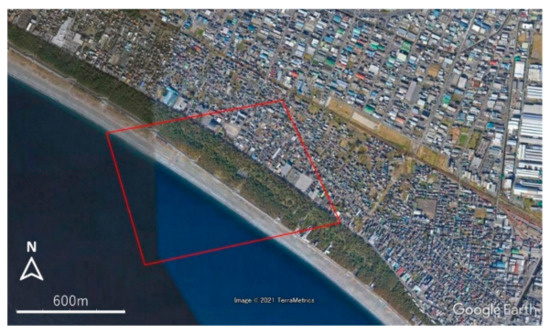
Figure 1.
An example of one of the target sites along the Fuji coast. The background image was obtained from Google Earth. The red rectangular frame indicates the area shown in Figure 2.
The present NN-based land–sea classification method uses the non-dimensional pixel value, Ci,j, obtained from the backscattering coefficient, B0,i,j, of the original SAR images. Here, i and j indicate the pixel coordinates of each image in the azimuth and range directions, respectively. Procedures for computation of Ci,j from B0,i,j are outlined as follows: first, the normalized backscattering coefficient, Bi,j, is determined as a function of B0,i,j by:
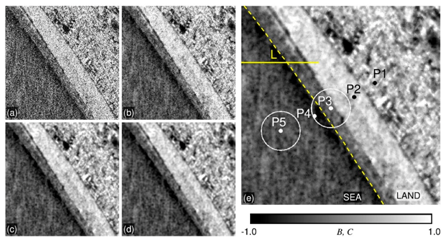
where ⟨B0⟩ and σB0 are the average and the standard deviation of B0 over each image, respectively. Figure 2a shows an example of the spatial distribution of the obtained Bi,j of the image along the Fuji coast, corresponding to the red rectangular domain shown in Figure 1. As seen in Figure 2a, we can distinguish the domains of sea and land, while both domains contain speckle noise. To remove the influence of this speckle noise and to highlight the contrast between sea and land, we applied the following bilateral filter [18] to obtain the pixel value, Ci,j:
where the weight on each pixel is determined by Gaussian kernels in the domains of the pixel coordinates and by the intensity difference of Bi,j with the corresponding scaling parameters σ1 and σ2. The bilateral filter effectively smooths the noise but preserves the edge of the image features. The relative importance of each Gaussian kernel is determined by the relative magnitude of σ1 and σ2. A larger σ1 smooths the larger features in space, while a larger σ2 enhances the relative smoothing effect of the intensity difference of the surrounding Bi,j. We applied σ1 = 3.0 pixels and investigated how the filtering characteristics depend on the quantity of σ2.
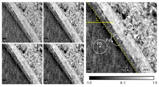
Figure 2.
Examples of modified SAR images of (a) normalized backscattering coefficient, B; (b–d) transferred C values with σ2 = 1, 3, and 10, respectively. (e) The enlarged image of (c) with indications of the shoreline (dashed line), line L, and points P1, P2, P3, P4, and P5. The area of the image is indicated by a rectangular frame in Figure 1.
Figure 2a shows the spatial distribution of B while Figure 2b–d shows those of C when σ2 = 1, 3, and 10, respectively. Figure 2e is the enlarged image of Figure 2c, with an indication of the shoreline; five referring points, P1, P2, P3, P4, and P5; and the line L, which are discussed later. Compared with the distribution of B shown in Figure 2a, the distribution of C with σ2 = 1 is slightly smoothed but contains a number of small black dots due to speckle noise. These black dots are mostly removed in Figure 2c,d with a larger σ2, but the sharpness of the image around the edge of the land–sea boundary appears to be deteriorated in Figure 2d when σ2 = 10.
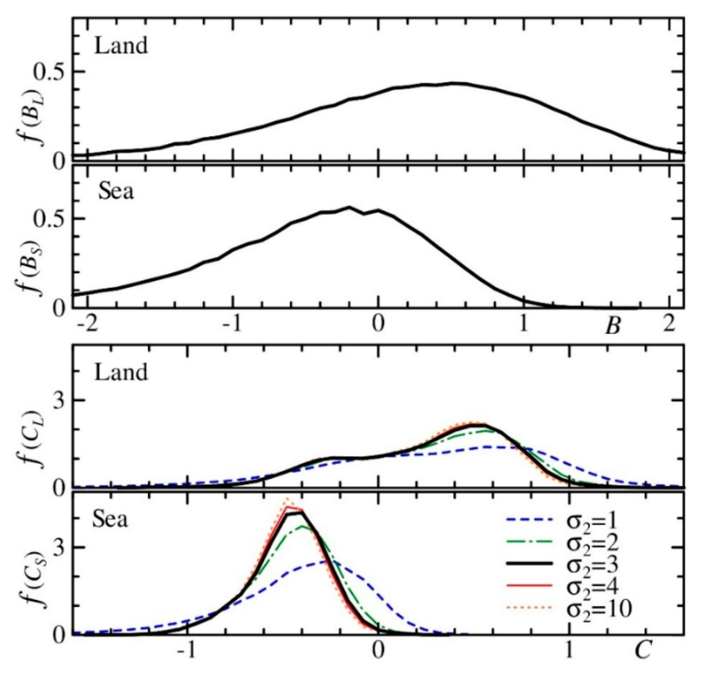
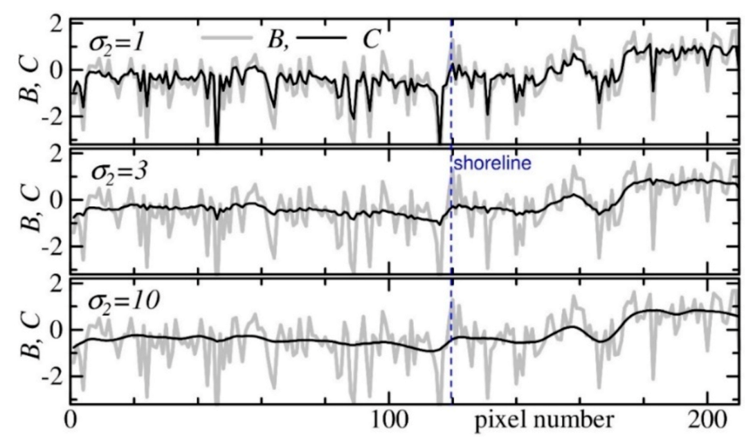
Figure 3 compares the probability distribution function of B and C on the land and the sea, f(BL), f(BS), f(CL), and f(CS), where L and S indicate the pixels on the land and sea domains, respectively. As seen in Figure 3, f(BL) and f(BS), shown in the top two panels, have broader profiles compared with f(CL) and f(CS), shown in the bottom two panels. Whereas the profile of f(BS) is located in the lower values of B compared with that of f(BL), these two profiles overlap with each other in a broad range of B. In contrast, the profile of f(CS) is much narrower than that of f(BS), and this narrower profile significantly decreases the range of overlap between f(CS) and f(CL). This feature clearly enhances the contrast between land and sea, indicating the advantage of the proposed bilateral filter for land–sea classification. The profile of f(CS) narrows with a larger σ2, but it tends to converge when σ2 is greater than three. Figure 4 compares B and C along the line L indicated in Figure 2e when σ2 = 1, 3, and 10. Figure 4 also shows the location of the shoreline along the line L. The distribution of B, shown in thick grey lines, shows noisy fluctuation, and these noises are smoothed in C. This smoothing effect also increases with σ2, and the variation in C across the shoreline also decreases with σ2. Based on these comparisons, we applied σ1 = σ2 = 3, which reasonably removed noise, but still preserved the clear change in C across the land–sea boundary.
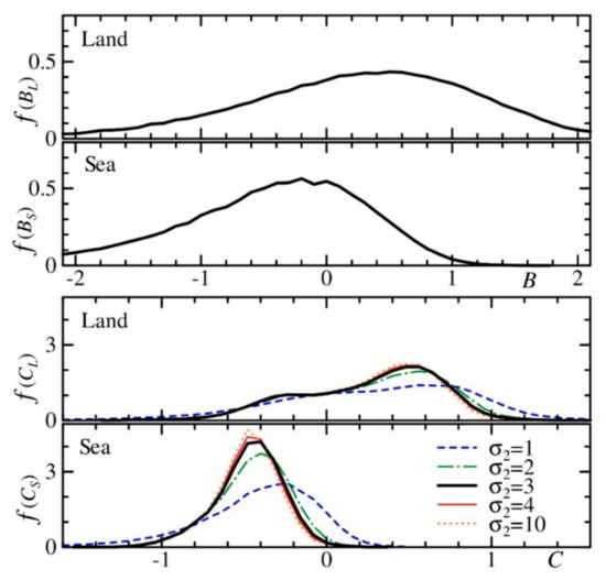
Figure 3.
Probability distribution function of B (top two panels) and C (bottom two panels) of pixels on land and sea.
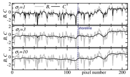
Figure 4.
Distribution of B (thick grey lines) and C (thin black lines) along the line L shown in Figure 2e. The top, middle, and the bottom panels show the same B but different C with σ2 = 1, 3, and 10, respectively.
3. Development of the NN-Based Land–Sea Classification Method
In this section, we describe the development of our NN-based method for land–sea classification of SAR images. A four-layer feedforward NN model, shown in Figure 5, was constructed for land–sea classification of the processed SAR imagery, with pixel values determined by C with σ1 = σ2 = 3. The input layer is determined by C values at the target pixel and the other surrounding pixels. We tested two different sets of input layers, which are introduced later. Through trial and error, the number of nodes of the two hidden layers was set to 50 and 20, and ReLU was applied as an activation function for both of the hidden layers. The NN outputs a single scalar. If the quantity of the output scalar is closer to unity than zero, then the target pixel is classified as a pixel on the land domain, and vice versa on the sea domain.
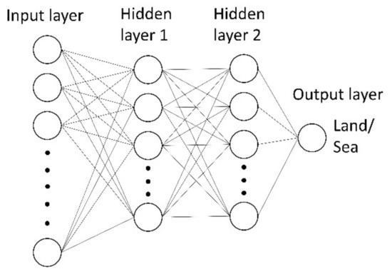
Figure 5.
Structure of the present neural network model.
3.1. Input Layer
This section describes how the input layer should be prepared for the present NN-based system. To investigate the characteristics of C values, two target pixels at P3 and P5, shown in Figure 2e, were selected, and the C values of the pixels surrounding each P3 and P5 were compared. These pixels at P3 and P5 have a similar C value though they are located on the land and sea, respectively. Figure 6 compares the C values of the pixels around P3 and P5.
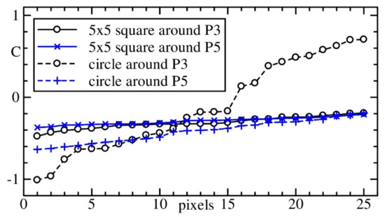
Figure 6.
Distributions of C values of 25 pixels in a 5 × 5 square and a circle around the target pixels, P3 and P5.
In Figure 6, solid lines show the distribution of C-values of 25 pixels within a 5 × 5 square, whose center corresponds to either P3 or P5. In Figure 6, a black line with a blank circle indicates the data around P3, while a blue line with a symbol of a diagonal cross indicates the data around P5. Here, the obtained 25 C values around each pixel were sorted in ascending order. The profiles of these lines are nearly identical to each other, suggesting that using C values of 25 pixels adjacent to the target pixel is not sufficient for reliable land–sea classification.
The dashed lines show the similar distributions of C values of the 25 pixels but along the circle with a radius of 50 pixels either from P3 or P5. Here, 25 pixels were selected along the circumference of the circle, shown in Figure 2e, with a constant interval, and the obtained C values were also sorted in ascending order. In contrast with solid lines, the dashed lines show clear differences between P3 and P5. These features suggest that the C values of pixels located at a certain distance from the target pixel provide important information for land–sea classification. The optimum radius of the circle around the target point may depend on the distance of the point from the land–boundary; thus, the use of multiple circles with different radii may enhance the robustness of the present NN-based land–sea classification method. Notably, the present method should be applicable to various images with arbitrary shoreline angles.
Taking these features into account, we tested two different methods, A and B, for the determination of the input layer of the proposed NN-based system. Both A and B consist of a single column of data of the C values of different pixels. In both A and B, the first 25 C values were extracted from the pixels within a 5 × 5 square with its center corresponding to the target pixel. The C value of the target pixel was placed at the top of the column and the C values of the remaining 24 pixels were placed after the first datum in ascending order. These 25 C values should represent the local features in the vicinity of the target pixel. The data, except for the target pixel, were sorted so that the prepared input layer would be independent of the shoreline angle in different images or rotation angles of the image. The first 25 data of the input layer were identical in both A and B. The two methods differ from each other in the later part of the input layer, which was extracted from the pixels along the circumference of concentric circles with the center at the target pixel and with different radii R of 3, 5, 7, 9, 10, 30, 50, 70, and 90 pixels.
In Method A, C values along each circle were sorted in ascending order and the values of the top 10%, 20%, 50%, 80%, and 90%, and their mean were placed. The total number of C values used for the input layer in Method A was, therefore, N = 25 + 6 × 9 = 79. Since all these data were sorted in each group of pixels of each concentric circle, the obtained layer was not affected by the shoreline angle of each image. However, Method A loses the information about the actual distribution of C values along the circumference of each circle.
To preserve the information of the actual distribution of C values, Method B applied the following procedures:
- Extract 60 C values of pixels in equal intervals along the circumference of the largest circle with the radius of R = 90 pixels, Ck, with k = 1,2, …60.
- Determine ⟨Ck⟩ as a moving average of Ck with a weight of a Gaussian kernel along the circumference of the circle.
- Find the point k, where the obtained ⟨Ck⟩ yields the maximum value along the circumference of the circle.
- Determine the initial angle as the angle between the northward direction and the direction from the center of the circle to the above-mentioned point.
- Use this initial angle to determine the initial point along each circle with different R.
- Extract the C values of the pixel along the circumference of each circle starting from the initial point in the clockwise direction in constant intervals.
- Place groups of these C values of each circle in ascending order of R.
Here, the number of C values extracted from each circle depended on R. We extracted 18, 30, 42, and 54 C values from circles with R = 3, 5, 7, and 9 pixels, respectively, and 60 C values from circles with R more than nine pixels. The total number of C values used in Method B was therefore N = 469.
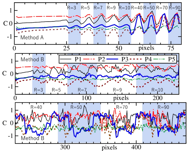
Figure 7 shows examples of the extracted input layer data at points, P1, P2, P3, P4, and P5, which are indicated in Figure 2e. Due to the sorting process, the input layer data in Method A show more systematic patterns than those in Method B. The data at P3 and P4, which are located at about the same distance from the shoreline boundary, significantly differ from each other in the first 25 pixels and in the data with lower R, but they are similar to each other with larger R. However, the input layer data at P3 and P5 are similar in the first 25 pixels and those with lower R, but they are clearly different in those with larger R. These contrasting differences and similarities in near and far fields of the target pixels should provide important information for the present land–sea classification method.
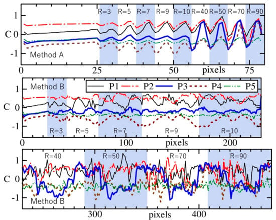
Figure 7.
Examples of the extracted data sequence of the input layer in Methods A and B at five different points, P1, P2, P3, P4, and P5, which are shown in Figure 2e. Legends of different lines are both for Methods A and B. P1, P2, and P3 are on the land, and P4 and P5 are on the sea. Shaded rectangles behind the figure indicate the range of the data extracted from different circles with different radius.
3.2. Training Samples
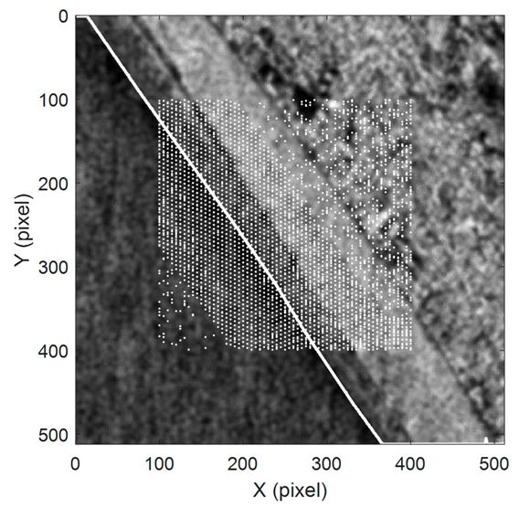
This section describes how the training samples were extracted from square grayscale images of Ci,j. Figure 8 shows an example of the distribution of the selected pixels, indicated by white dots in the image. As shown in Figure 8, training samples were extracted from the 300 × 300 square domains in the middle of 512 × 512 images because the input data for the proposed NN-based system require the pixel information not only at the target pixel but also for the pixels a certain distance away from the target pixel. First, 60 lines parallel to the eye-detected shoreline were selected in each image. These parallel lines were placed on both sides of the shoreline with an interval of 5 pixels in the shore-normal direction. Along each line, the target pixels were also selected with an interval of 5 pixels. This minimum distance, 5 pixels, was determined so that the sampling points were away from the land-sea boundary since the error of eye-detected shoreline location may result in wrong land-sea classification in the vicinity of the land-sea boundary. Additional pixels were randomly selected within the 300 × 300 domain to ensure that the number of pixel samples in each image, 3660, was identical to each other. Through these procedures, in total, we obtained 264,523 samples from the land and 229,577 samples from the sea.
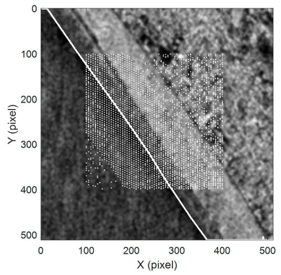
Figure 8.
Distribution of training samples, shown in white dots, on an example image of the Fuji coast.
3.3. Training Procedures
Training data were obtained from 97 images, which is about 72% of the entire 135 images used in this study. These training images were randomly selected from all the images. We applied Adam as the optimization algorithm with a batch size of 1000 and adopted the early stopping method to avoid overfitting. Through the training, we confirmed that the computed cross-entropy loss was quickly reduced with the increase in epoch number and converged to a sufficiently low quantity, 0.03, in both Methods A and B. The accuracy of land-sea classification, defined as the rate of correctly classified pixels over the entire number of pixels, was also as high as 0.99 in both cases.
3.4. Testing Results
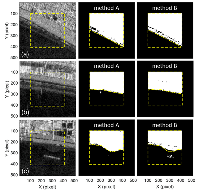
The developed NN model was tested using the remaining 38 images. Figure 9 shows examples of the classification results. These panels show that most of the pixels were correctly classified into land and sea, and the land–sea boundary was easily detected from these binarized images. However, these images still contain a certain number of pixels that were misclassified as a pixel in the sea while it was on land. In both methods, such misclassification of land pixels appeared for relatively dark pixels, i.e., low C value. The shoreline in Figure 9c has a convex profile behind a detached breakwater. In this image, the result of Method A, shown in the middle panel, exhibits better performance in land-sea classification around the tip of the convex beach shape.
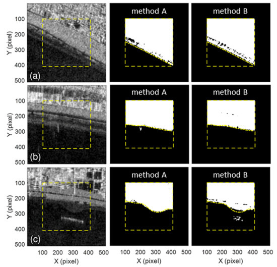
Figure 9.
Examples of the classification results produced by the proposed NN model. Panels in the left column show the modified SAR image with a square frame with a yellow dashed line indicating a 310 × 310 square domain in which the proposed NN model was applied. The panels in the middle and right columns show the results of land (white) and sea (black) classification using Methods A and B, respectively. Yellow curved lines in these panels indicate the eye-detected shoreline. Pixel size is around 1.4 m in the Y (azimuth) direction and 1.9 m in the X (range) direction.
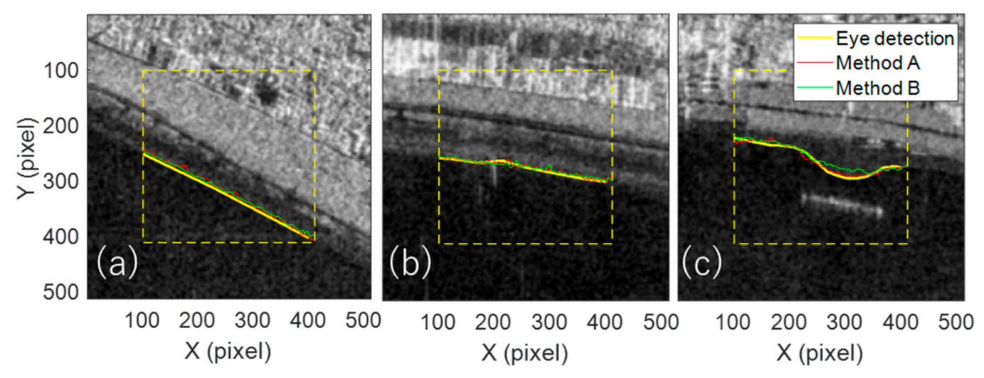
Since the final goal of the proposed NN-based method is the extraction of shoreline locations, the performance of the system was also tested through comparisons of extracted shorelines. We applied the edge detection technique presented by Tajima et al. [7], based on the two-dimensional horizontal wavelet obtained as a product of the Haar function in the cross-shore direction and the Gaussian-type weight function in the alongshore direction. Figure 10 shows examples of the extracted shorelines from the binarized images shown in Figure 9 for both Methods A (red) and B (green). For comparison, Figure 10 also shows the eye-detected shoreline using a yellow solid line.
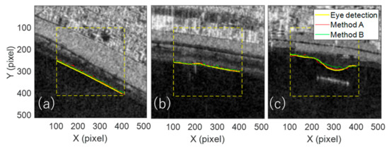
Figure 10.
Comparisons of shoreline locations extracted through the proposed NN-based model and through eye detection. Three images, (a–c), correspond to those shown in Figure 9.
The eye-detected shoreline was obtained through the following procedures. First, the image with a size of 25 × 25 cm was displayed on the computer monitor. The pixel size of the displayed image was about 0.5 mm on the monitor. In this image, pixel coordinates of the shoreline were detected by eye as a boundary between the brighter land domain and the darker sea domain. Tajima et al. [7] conducted the same procedures to obtain the eye-detected shoreline, and showed that the eye-detected shoreline agreed well with the measured shoreline within the error of 5 m. It should be noted that all the eye detections in this study and in Tajima et al. [7] were conducted by the same person.
Overall, as seen in these figures in Figure 10, the shoreline extracted from the binarized images agrees well with the eye-detected shoreline. The extracted shoreline in Figure 10c based on Method B is located away from the eye-detected shoreline in the landward direction around the tip of the convex profile of the shoreline. This is because the proposed NN model with Method B misclassified land pixels as sea pixels around the tip of the convex profile.
It should also be noted that the shoreline locations obtained either by the present NN-based method or by the above-mentioned eye-detection are the ones for the seawater level at the time of satellite observation. The shoreline location at the specified sea level, such as the mean sea level, can be estimated by the information of the cross-shore bed slope around the shoreline and the seawater level at the time of observation. Tajima et al. [7] showed that the increasing number of shoreline observations significantly reduce the error of the estimated shoreline location at the specified sea level. This feature also highlights the advantage of the frequent monitoring enabled by the present shoreline detection technique based on SAR imagery.
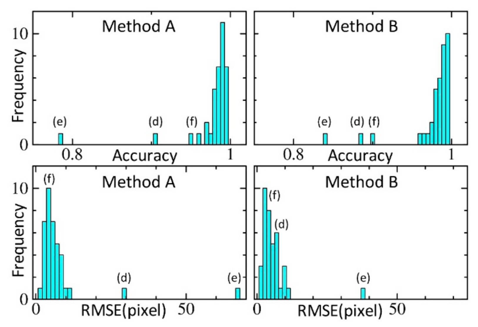
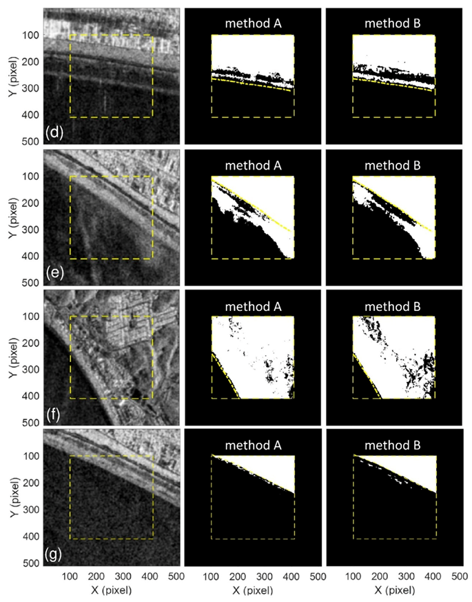
Finally, a similar comparison was performed for all the 38 test images. Figure 11 shows the histograms of the accuracy of land–sea classification and the root mean square errors (RMSEs) between the estimated and eye-detected shoreline locations for both Methods A and B. In both Methods A and B, accuracy was higher than 0.95 in 35 of 38 images. Figure 9a–c shows images with high accuracy. Figure 12 shows the classification results of three images, (d), (e) and (f), with relatively low accuracy. In images (d) and (f), for example, most of the misclassified pixels are on land, where the value of C is relatively low. These misclassifications are away from the shoreline, and thus have little influence on the extracted shoreline positions. In Figure 12, image (f), for example, the RMSEs of the shoreline location are 6.3 and 5.1 pixels in Methods A and B, respectively. These RMSEs are within the range of RMSEs of the other images, which yielded higher accuracy than 0.95. In Figure 12, image (d), some pixels are also misclassified as sea pixels in the vicinity of the shoreline with Method A. This misclassification clearly increases the RMSE in Method A, as seen in Figure 11. In Figure 12, image (d), a darker area is observed just on the land side of the shoreline. Under this condition, the relative importance of the spatial distribution information of C values, omitted in Method A, may be of importance.

Figure 11.
Histogram of the accuracy of land–sea classification (top) and RMSE of the extracted shoreline position (bottom) for Method A (left) and Method B (right). In the figure, (d), (e) and (f) indicate the accuracy and RMSE of images (d), (e) and (f) shown in Figure 12.
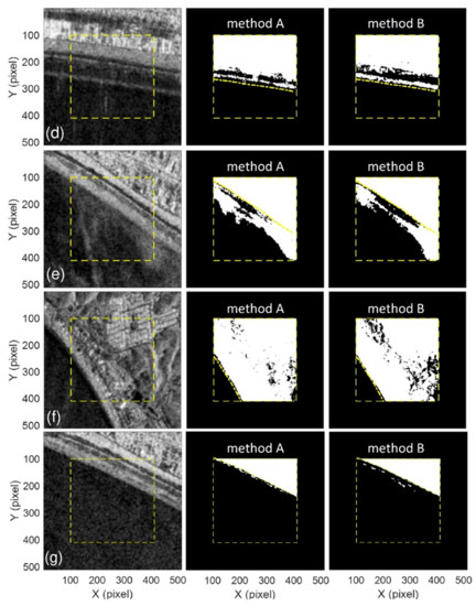
Figure 12.
Examples of the classification results produced by the proposed NN model. The definitions of these panels are the same as those in Figure 9, but these panels are for different images, (d–f), which yielded relatively low-accuracy land–sea classification, as indicated in Figure 11. The image (g) is extracted from the same site as (e), but at a different observation time.
In Figure 12, image (e), both Methods A and B misclassify pixels in the sea as a land pixel near the shore. As seen in Figure 12, image (e), relatively high C values are recorded near the shore. These high C values on the sea surface may be because the sea surface was rough when this SAR image was recorded. Figure 12, image (g) shows the same classification results but for the different images at the site same as (e) but at different observation times. Accuracies of the classification of this image (g) were 0.99 for both Methods A and B, and RMSEs of detected shoreline location were 3.9 and 1.5 for Methods A and B. Clearly, the proposed system showed different classification performance of the images along the same coast recorded at different times. As discussed by Wu et al. [6] and Tajima et al. [7], the selection of images appropriate for land–sea classification considering the influence of the sea surface condition at the time of satellite observation is one of important procedures for reliable shoreline extraction from SAR scenes.
4. Application of the Present System to the Other Coasts
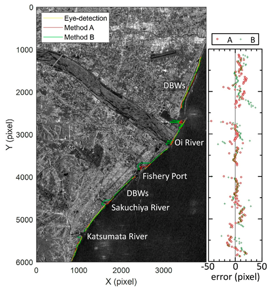
This section describes our application of the developed NN-based land–sea classification method to two other coasts in Japan, which were not used for the training of the proposed NN model: the Suruga coast in the Shizuoka prefecture and the Shirimi-hama coast located in the Mie prefecture. Both coasts have long and mildly curving beaches. The left panels of Figure 13 and Figure 14 show the grayscale images based on the original SAR scenes for both coasts with three solid lines in different colors indicating the shoreline extracted from eye-detection (yellow), and from the proposed method with input layers based on Method A (red) and B (green). Note that these two coasts face eastward, whereas all the coasts used for training faced southward or southwestward. The right panels of Figure 13 and Figure 14 show the alongshore distributions of the differences in the shoreline locations in the shore-normal direction between the one based on eye-detection and the others extracted from the present system with Methods A (red circle) and B (green cross). In the panel, the vertical axis is pixel coordinates in the north–south direction, corresponding to that of the left panel. The horizontal axis is the difference in the shoreline location in the shore-normal direction with the unit of pixels.
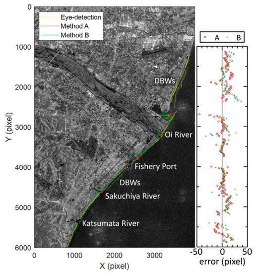
Figure 13.
Grayscale image of the Suruga coast with extracted shorelines (left) and differences in the shoreline position between that extracted from eye-detection and the others from the NN models (right).
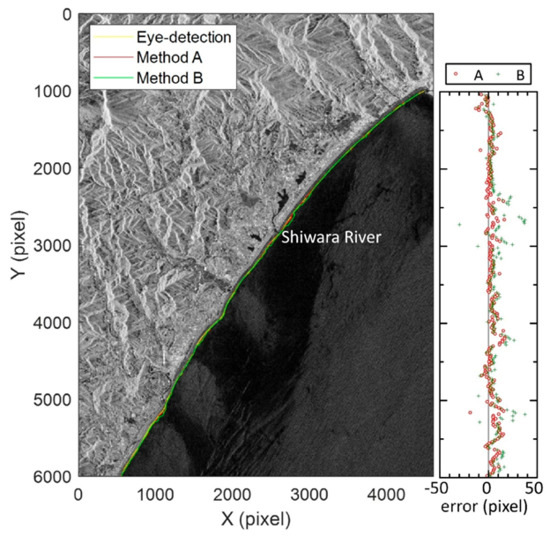
Figure 14.
Grayscale image of the Shirimi-hama coast with extracted shorelines (left) and the differences in the shoreline position between the eye-detected one and those from the NN models (right).
The coastal area shown in Figure 13 has a number of detached breakwaters (DBWs), a fishery port, the Oi River mouth, and two other small river mouths. The proposed NN-based system successfully extracted the shoreline behind the DBWs with both Methods A and B. The system also extracted the shoreline of the sand spit developed at the Oi River mouth, but it partially failed to detect the shoreline around the north tip of the sand spit. Method B also failed to detect a part of the shoreline around the river mouth and a fishery port where relatively dark pixels were partially distributed on the land. Method A performed relatively better in shoreline detection around these river mouths and fishery port.
In contrast with the Suruga coast, the Shichirimi-hama coast, shown in Figure 14, has no coastal structures and has less-complex patterns of C values on the land. The proposed NN-based system, therefore, showed fairly accurate shoreline extraction performance using both Methods A and B. The difference in the shoreline position between eye-detection and the proposed system was less than 10 pixels along most of the coast. A relatively large difference was found using Method B at around Y = 2700 and 5200 pixels, which have a lagoon and estuary near the shore, respectively.
These results support the reasonable applicability of the proposed NN-based system for relatively accurate shoreline detection based on SAR images that were not used for the training of the system. The system can be applied to arbitrary SAR images without site-specific information and calibration parameters. In addition, the model can be further trained through the accumulation of accurate and reliable training data.
Due to the limited number of tests, it is difficult to conclude the relative merits of these two methods. Overall, Method A requires less input layer data, and is thus slightly more efficient in computation. Method A appears to yield slightly more accurate detection results of the shoreline location, while Method B shows higher accuracy behind the detached breakwaters at around Y = 1700 pixels in Figure 13.
5. Conclusions
In this study, we developed an automatic NN-based shoreline detection method based on SAR images. The proposed NN model first classifies the pixels into land and sea. The feedforward NN model consists of four layers: an input layer, two hidden layers, and an output layer. The input layer is based on the pixel values of the SAR image. The backscattering coefficients of original SAR images are transferred to C values after normalization and application of a bilateral filter. We confirmed that the present bilateral filter reasonably removes speckle noise and enhances the contrast of pixels between land and sea. Based on the obtained C values, the input layer was prepared using two different methods, A and B. In both methods, the C values of the 25 pixels closest to the target pixel were first placed in ascending order. The two methods differed from each other in the later part of the input layer. Ignoring the spatial distribution of C values, Method A used the sorted representative C values along the circumference of several concentric circles with its center at the target circle. Method B uses the same concentric circles, and simply extracts the C values along each circumference in uniform intervals in the clockwise direction. In this manner, the input layer of Method B is lengthy but preserves the spatial distribution information of the C values.
Both Methods A and B showed good classification accuracy, higher than 0.95, in most of the test images; we found that the accuracy deteriorated under certain conditions such as rough sea surface and distribution of relatively low C values on the land due to a very smooth ground surface or inland waters such as estuaries and lagoons. Finally, the edge detection technique based on the two-dimensional horizontal wavelet of the product of Haar and Gaussian functions was applied to binary images obtained through the proposed NN-based model. The obtained shoreline location was then compared with the one obtained by eye detection. We found that the RMSEs of the shoreline position were generally less than 10 pixels using both Methods A and B. The performance of the two methods is nearly the same but Method A is simpler and shows slightly better extraction skill when relatively low C values are distributed on the land due to the existence of ports, estuaries, and lagoons. Method B shows slightly better performance behind detached breakwaters. Further model tests using different SAR scenes are necessary for the evaluation of the relative merits of these two methods. Overall, however, the relatively high accuracy and low computational cost support the advantages of the proposed method for shoreline detection and monitoring.
Author Contributions
Conceptualization, Y.T.; methodology, Y.T. and L.W.; validation, L.W. and K.W.; investigation, Y.T. and L.W.; resources, Y.T. and K.W.; writing—original draft preparation, Y.T.; writing—review and editing, Y.T. and L.W.; visualization, Y.T. and L.W.; supervision, Y.T. All authors have read and agreed to the published version of the manuscript.
Funding
A part of this study was supported by the “Grant for R&D on River and Sabo Engineering Technologies, 2016–2017” provided by the Ministry of Land, Infrastructure, Transport and Tourism (MLIT), Japan.
Data Availability Statement
Data sharing is not applicable to this article due to privacy.
Conflicts of Interest
The authors declare no conflict of interest.
References
- Boak, E.H.; Turner, I.L. Shoreline definition and detection: A review. J. Coast. Res. 2005, 21, 688–703. [Google Scholar] [CrossRef]
- Mentaschi, L.; Vousdoukas, M.I.; Pekel, J.-F.; Voukouvalas, E.; Feyen, L. Global long-term observations of coastal erosion and accretion. Sci. Rep. 2018, 8. [Google Scholar] [CrossRef] [PubMed]
- Hussain, M.A.; Tajima, Y.; Gunasekara, K.; Rana, S.; Hasan, R. Recent coastline changes at the eastern part of the Meghna Estuary using PALSAR and Landsat images. IOP Conf. Ser. Earth Environ. Sci. 2014, 20, 012047. [Google Scholar] [CrossRef]
- Lee, J.S.; Grunes, M.R.; de Grandi, G. Polarimetric SAR speckle filtering and its implication for classification. IEEE Trans. Geosci. Remote Sens. 1999, 37, 2363–2373. [Google Scholar] [CrossRef]
- Mason, D.C.; Davenport, I.J. Accurate and efficient determination of the shoreline in ERS-1 SAR images. IEEE Trans. Geosci. Remote Sens. 1996, 34, 1243–1253. [Google Scholar] [CrossRef]
- Wu, L.H.; Tajima, Y.; Yamanaka, Y.; Shimozono, T.; Sato, S. Study on characteristics of synthetic aperture radar (SAR) imagery around the coast for shoreline detection. Coast. Eng. J. 2019, 61, 152–170. [Google Scholar] [CrossRef]
- Tajima, Y.; Wu, L.H.; Fuse, T.; Shimozono, T.; Sato, S. Study on shoreline monitoring system based on satellite SAR imagery. Coast. Eng. J. 2019, 61, 401–421. [Google Scholar] [CrossRef]
- Liu, H.; Jezek, K.C. Automated extraction of coastline from satellite imagery by integrating canny edge detection and locally adaptive thresholding methods. Int. J. Remote Sens. 2004, 25, 937–958. [Google Scholar] [CrossRef]
- Wang, Y.; Allen, T.R. Estuarine shoreline change detection using Japanese ALOS PALSAR HH and JERS-1 L-HH SAR data in the Albemarle-Pamlico sounds, North Carolina, USA. Int. J. Remote Sens. 2008, 29, 4429–4442. [Google Scholar] [CrossRef]
- Buono, A.; Nunziata, F.; Mascolo, L.; Migliaccio, M. A multipolarization analysis of coastline extraction using X-band COSMO-SkyMed SAR Data. IEEE J. Sel. Top. Appl. Earth Obs. Remote Sens. 2014, 7, 2811–2820. [Google Scholar] [CrossRef]
- Al Fugura, A.; Billa, L.; Pradhan, B. Semi-automated procedures for shoreline extraction using single RADARSAT-1 SAR image. Estuar. Coast. Shelf Sci. 2011, 95, 395–400. [Google Scholar] [CrossRef]
- Sheng, G.F.; Yang, W.; Deng, X.P.; He, C.; Cao, Y.F.; Sun, H. Coastline detection in synthetic aperture radar (SAR) images by integrating watershed transformation and controllable Gradient Vector Flow (GVF) snake model. IEEE J. Ocean. Eng. 2012, 37, 375–383. [Google Scholar] [CrossRef]
- Zhang, D.; Vangool, L.; Oosterlinck, A. Coastline detection for SAR images. In Proceedings of the IEEE International Symposium on Geoscience and Remote Sensing, Pasadena, CA, USA, 8–12 August 1994; IEEE: New York, NY, USA, 1994; Volumes 1–4, pp. 2134–2136. [Google Scholar]
- Ding, X.W.; Li, X.F. Coastalline detection in SAR images using multiscale normalized cut segmentation. In Proceedings of the IEEE International Symposium on Geoscience and Remote Sensing, Quebec City, QC, Canada, 13–18 July 2014. [Google Scholar]
- Nunziata, F.; Buono, A.; Migliaccio, M.; Benassai, G. Dual-polarimetric C- and X-Band SAR data for coastline extraction. IEEE J. Sel. Top. Appl. Earth Obs. Remote Sens. 2016, 9, 4921–4928. [Google Scholar] [CrossRef]
- Vandebroek, E.; Lindenbergh, R.; van Leijen, F.; de Schipper, M.; de Vries, S.; Hanssen, R. Semi-automated monitoring of a mega-scale beach nourishment using high-resolution TerraSAR-X satellite data. Remote Sens. 2017, 9, 653. [Google Scholar] [CrossRef]
- Fuse, T.; Ohkura, T. Development of shoreline extraction method based on spatial pattern analysis of satellite SAR images. Remote Sens. 2018, 10, 1361. [Google Scholar] [CrossRef]
- Tomasi, C.; Manduchi, R. Bilateral filtering for gray and color images. In Proceedings of the 6th International Conference on Computer Vision, Bombay, India, 7 January 1998; pp. 839–846. [Google Scholar] [CrossRef]
Publisher’s Note: MDPI stays neutral with regard to jurisdictional claims in published maps and institutional affiliations. |
© 2021 by the authors. Licensee MDPI, Basel, Switzerland. This article is an open access article distributed under the terms and conditions of the Creative Commons Attribution (CC BY) license (https://creativecommons.org/licenses/by/4.0/).


