Article

Monitoring Wet Snow Over an Alpine Region Using Sentinel-1 Observations

1
Univ. Grenoble Alpes, Université de Toulouse, Météo-France, CNRS, CNRM, Centre d’Études de la Neige, 38000 Grenoble, France
2
Météo-France, DirOP, Cellule Montagne Nivologie, 38400 Saint Martin d’Heres, France
3
Centre Nat. d’Etudes Spatiales, 31400 Toulouse, France
4
Université de Toulouse, CNRS/CNES/IRD/INRA/UPS, 31400 Toulouse, France
*
Author to whom correspondence should be addressed.
Remote Sens. 2021, 13(3), 381; https://doi.org/10.3390/rs13030381
Submission received: 23 December 2020 / Revised: 12 January 2021 / Accepted: 19 January 2021 / Published: 22 January 2021
(This article belongs to the Special Issue Advances in Spaceborne SAR – Technology and Applications)

Abstract

:
The main objective of this study was to monitor wet snow conditions from Sentinel-1 over a season, to examine its variation over time by cross-checking wet snow with independent snow and weather estimates, and to study its distribution taking into account terrain characteristics such as elevation, orientation, and slope. One of our motivations was to derive useful representations of daily or seasonal snow changes that would help to easily identify wet snow elevations and determine melt-out days in an area of interest. In this work, a well-known approach in the literature is used to estimate the extent of wet snow cover continuously over a season and an analysis of the influence of complex mountain topography on snow distribution is proposed taking into account altitude, slope, and aspect of the terrain. The Sentinel-1 wet snow extent product was compared with Sentinel-2 snow products for cloud free scenes. We show that while there are good agreements between the two satellite products, differences exist, especially in areas of forests and glaciers where snow is underestimated. This underestimation must be considered alongside the areas of geometric distortion that were excluded from our study. We analysed retrievals at the scale of our study area by examining wet snow Altitude–Orientation diagrams for different classes of slopes and also wet snow Altitude–Time diagrams for different classes of orientations. We have shown that this type of representation is very useful to get an overview of the snow distribution as it allows to identify very easily wet snow lines for different orientations. For an orientation of interest, the Altitude–Time diagrams can be used to track the evolution of snow to locate altitudes and dates of snow loss. We also show that ascending/descending Sentinel-1 image time series are complementary to monitor wet snow over the French alpine areas to highlight wet snow altitude ranges and identify melt-out days. Links have also been made between Sentinel-1 responses (wet snow) and snow/meteorological events carefully listed over the entire 2017–2018 season.

Graphical Abstract

1. Introduction

In alpine regions, monitoring the spatial and temporal variations of snow conditions is a key element for many applications such as hydrology, mountain ecosystems, meteorological, and avalanche forecasting. Mapping wet snow is a critical input for wet snow avalanche forecasts. Wet snow avalanches occur when melt water or rain penetrate the snowpack, leading to increased instability of the snowpack, but are difficult to predict and estimate, even a posteriori [1]. Furthermore, assessing the amount of snow, its evolution over time, and particularly the start date of snowmelt is critical to optimize hydro-power production and to anticipate flood risk. The melt-out date of the seasonal snow cover plays an important role in mountain ecosystems [2].
Remote sensing allows monitoring of seasonal snow everywhere and as often as possible according to the observation constraints of satellite sensors, although specific challenges need to be addressed such as separating the contributions of snow and canopy in forests, the need for adequate pre-processing of observations in complex terrain and the requirements for satellite product evaluation through in situ observations [3]. Sentinel-1 satellites provide C-band synthetic aperture radar (SAR) data at unprecedented temporal and spatial resolutions and are able to detect the presence of wet snow [4,5,6]. This makes it possible to contribute to monitoring seasonal snow in the mountains at high resolution [7]. Sentinel-1 observation time series were studied by [8] to infer information about snowmelt dynamics. These data were also used by [9] to map snow depth in the Northern Hemisphere mountains at 1 km 2 resolution using change detection method. In the study of [10], the authors evaluated backscatter numerical simulations at C-band over mountains using a chain of models composed of the SAFRAN meteorological reanalysis, the Crocus snowpack model, and the radiative transfer model Microwave Emission Model for Layered Snowpacks (MEMLS3&a). The authors showed that there is good agreement between Sentinel-1 observations and simulations under snow-free or dry snow conditions. Under wet snow conditions, a bias between observations and simulations was noted although the changes in time and space are well correlated. A review about snow retrievals from SAR data is given in [11]. For C-band co-polarized measurements, there is low absorption or scattering of the signal by dry snow, whereas the signal undergoes high absorption and reflection by wet snow. In the study of [12], the authors have shown that polarimetric information from multi-frequency (L- and C-bands) and multi-temporal SAR data can be successfully used to map the extent of dry snow in alpine areas. For a wet snowpack, surface refreezing would result in a strong volumetric scattering of the coarse grains of the refrozen layer and therefore an increase in backscattering ([13]). Snow volume scattering is more noticeable in cross-polarization with a gradual increase in backscatter with snow accumulation, a decrease in backscatter is generally observed for wet snow probably caused by absorption and reflection processes ([9]). Wet snow detection methods usually rely on change detection approach using an image ratio to compare two images (wet snow backscatters are generally lower than dry snow or soil backscatters). The ratio between two images with and without snow is computed for the same study area and a threshold is applied to derive a snow mask [14]. Algorithmic improvements have been designed [5,7] to better account for minimum and maximum values of snow backscatter and for an optimized choice of reference images. In addition to snow parameters, surface roughness and local incidence angle also contribute to the complex relationship between backscatter and snow, resulting in positive or negative correlations depending on the situation ([13,15,16]). The relationship between incidence angles and co/cross polarizations at C-band was investigated [17] in order to identify wet snow-covered surfaces. The wet snow and soil separation was shown to be easiest with incidence angle values close to 45 [18]. The study of [4] used Sentinel-1 images with a −2 dB threshold by combining the two available VV and VH polarizations. A stochastic approach was used [19] to map wet snow probability occurrences. Data fusion methods have also been used to combine snow information from optical images and from SAR images ([20,21]).
The main objective of this study was to monitor wet snow conditions from Sentinel-1 over a season, to examine its variation over time by cross-checking wet snow with independent snow and weather estimates, and to study its distribution taking into account terrain characteristics such as elevation, orientation, and slope. One of our motivations was to derive useful representations of daily or seasonal snow changes that would help to easily identify wet snow elevations and determine melt-out days in an area of interest.
This article relies on the method described in [4] and combines Sentinel-1 VV/VH polarizations to monitor wet snow in a steep alpine mountainous area during a 7 month period (62 Sentinel-1 scenes with ascending and descending modes). The study of [4] uses 3 Sentinel-1 descending orbit images (of June 2015) to derive wet snow maps. The robustness of the wet snow retrieval approach is studied by evaluating the performances of the wet snow detection method taking into account terrain characteristics (elevation, slopes, aspects) and meteorological events during the time period of December 2017 to June 2018 over an alpine area. The studied season is characterized by exceptional snow cover following extremely heavy precipitation events associated with temperatures significantly below average, except in January, exceptionally warm. Snow conditions were quite variable depending on the altitude with ordinary snow conditions below 1200 m, remarkable snow conditions from 1500 m, and exceptional snow conditions from 1800 m approximately [22]. Whenever possible, comparisons between Sentinel-1 and Sentinel-2 snow products were also performed.
Data and models used in this study are described in Section 2. Results are provided in Section 3, while Section 4 provides discussion and conclusion statements.

2. Data and Method

2.1. Location and Time Period

The area under investigation is located in the French Alps, as shown on Figure 1. This figure also shows the elevation, aspect, and slope distribution of the study area. The spatial coverage of relevant Sentinel-1 orbits for our study area is also plotted. Our area is a quite heterogeneous alpine zone with complex topography and with terrain mainly dominated by north/south aspects. It has an area of 2310 km 2 with several land cover types including forests, bare ground, glaciers, and wetlands (as shown on Figure 1 using 25 m resolution land cover products from the CORINE Land Cover (CLC) European database). The time period of this study ranges from December 2017 to June 2018. This corresponds to highly disturbed meteorological and snow conditions in the European Alps and particularly the French Alps [22,23].

2.2. Sentinel-1 Data

We use backscatter coefficients at C-band from SAR observations on board Sentinel-1 missions launched by the European Space Agency (ESA) within the Copernicus Program. Sentinel-1 mission consists of a constellation of two satellites, Sentinel-1A and Sentinel-1B, which are 180 orbit apart, which allow continuous observations of the French Alps every 6 days. Sentinel-1A and Sentinel-1B were launched in April 2014 and April 2016 respectively. Sentinel-1 has a side-looking imaging geometry, so that images are subject to geometry-induced radiometric distortions (shadow, layover, and foreshortening effects). In case of foreshortening, mountain slopes facing the sensor are compressed in a few image pixels which appear bright. Layover effect, it is an extreme case of foreshortening; it occurs in cases where the top of the mountain is closer to the sensor than the bottom. Shadow areas correspond to the hidden parts of the radar beam. This phenomenon occurs when the target is obscured by an obstacle. Layover, foreshortening, and shadow regions are usually simulated using digital elevation models and sensor acquisition parameters (see for instance [24,25]).
We used Level-1 Ground Range Detected (GRD) products available from the ESA web site (https://scihub.copernicus.eu/dhus/). Sentinel-1 data have a spatial resolution of 20 m in both VV and VH polarizations. We use Sentinel-1 relative orbits A161 (ascending) and D139 (descending), which are relevant for our test site and study period. SAR data have been processed using the ESA Sentinel-1 Toolbox (SNAP). For preprocessing SAR data, the following SNAP software operators are used in the following order: (1) “Apply orbit file” to updated orbit metadata with a more precise orbit file, (2) “GRD border noise removal”, to remove low intensity noise and invalid data on scene edges, (3) “Thermal noise removal” to help reducing noise effects a noise look-up table, (4) “Radiometric calibration” to compute backscatter intensity using sensor calibration parameters in the GRD metadata, (5) “Speckle Filtering” to reduce the data inherent salt and pepper like textures (using refined Frost filter [26]), and (6) “Terrain correction” to convert data from ground range geometry to sigma0 using the National Institute for Geographic and Forestry Information (IGN) 25 m Digital elevation model. Areas of shadow, layover, and foreshortening areas were identified for each orbit using the SNAP module “SAR Simulation Terrain Correction”. Since no specific corrections have been made to correct or attenuate layover/foreshortening effects (see for instance methods proposed by [27,28]), shadow, layover, foreshortening areas have been excluded. Note that the use of such methods would correct the geometry of the scene as well as its radiometry by normalizing the backscatter to the local illuminated area as seen by the sensor without using an ellipsoid-model-based incidence angle as we get from terrain correction. A series of 62 Sentinel-1 images from ascending and descending orbits were used, and are listed in Table 1 and Table 2. We use the Theia snow products derived from Sentinel-2 data when available over our test zone (cloud free situations) [29]. The Sentinel-2 mission developed by the European Space Agency (ESA) is composed of two satellites (Sentinel-2A and Sentinel-2B) operating in the same orbit (786 km) launched in 2015 and in 2017, respectively. These snow retrieval products are developed by CNES and CESBIO and are available from the Theia website (https://theia.cnes.fr). Sentinel-2 snow retrieval products used in this study are listed in Table 1 and Table 2. Sentinel-2 snow retrieval products are used as a reference to evaluate Sentinel-1 derived wet snow maps. We would like to emphasize that the Sentinel-2 snow retrievals refer to snow extent whereby dry versus wet is not distinguished, while Sentinel-1 only detects wet snow, so the comparison is not between two identical snow retrievals. In addition, significant differences between the two snow products could be caused by the different satellite overpass times.

2.3. Methods

Several Sentinel-1 pre-processing steps are necessary before computing wet snow maps. A workflow within the ESA SNAP toolbox has been designed to automatically process all Sentinel-1 scenes (data of each orbit tracks has been processed separately). The workflow includes precise orbit data update, calibration of images, the speckle reduction using Frost filter, co-registration of images and terrain correction. For each orbit track, a summer image was selected as a master scene (24–25 August 2017 for D139 and A161, respectively). SAR local incidence angles as well as shadow/layover/foreshortening binary masks were computed using the IGN 25 m DEM. Backscatter ratio values of the winter image versus the reference one were computed for tracks D139 and A161 for the VV and the VH polarizations. We then merged VV and VH ratio to compute a combined single channel Rc using values of the local incidence angle following the method described in [4]:
R c = W R v h + ( 1 W ) R v v
where W varies with respect to the local incidence angle. Rvv is VV-polarized ratio between snow image and the summer reference. Rvh is VH-polarized ratio between snow image and the summer reference. A threshold of −2 dB was then applied to compute ascending/descending wet snow maps. Sentinel-1 wet snow products were also filtered to reduce single outlayer pixels. Ascending and descending products were used separately or merged (called S1 Combined hereafter) to observe different sides of mountains. The wet snow binary images from the descending orbit of day D and the ascending orbit of day D + 1 were combined into a single wet snow product, preserving wet snow detection information regardless of orbit direction. The combined product is binary and contains the following values: 0 if bare ground or dry snow, 1 if wet snow is detected within 48 h by one or both orbits. Note that all our images are perfectly co-located and have the same number of pixels.

2.4. Elements About Snow and Meteorological Conditions

S1 observations are sensitive to the amount of liquid water in the seasonal snowpack, whose variations in time and space are particularly difficult to quantify (e.g., [30]). Specific situations of interest for the evaluation of S1 observations in this respect, thus include rain events reaching above the snowline (Rain-On-Snow events: ROSE) ([31]), and melt events (ME) [32]), when liquid water forms close to the snow surface due to the surface energy balance. While ROSE are affected by spatial variations in precipitation and rain/snow transition, melt is much controlled by slope aspect, inclination and elevation in link with incoming short wave radiation and orographic gradients. While the penetration of liquid water in a dry snowpack is rapid and highly heterogeneous ([33]), both along slope-parallel and slope-perpendicular dimensions ([34]), this small-scale heterogeneity lowers when the snowpack is wet. As a result of spring diurnal cycles, wet surface snow layers or thin snowpacks can also refreeze over night (20 to 40 cm of total refreezing is common in one night, especially at an early stage of humidification). Thus, a thin or only moderately wet snowpack may be dry or wet for the same day depending on the time of observation.
In this study, S1 and S2-based snow products are analyzed with respect to snow conditions estimated every day by Météo-France snow and avalanche forecasters and provided in snow and avalanche bulletins for the Oisans massif (this massif is representative of our test area). The forecast bulletins provide information on snow, weather conditions such as snowfall, rainfall, wind, and the corresponding avalanche risk using the European Avalanche Danger Scale. On all the Northern Alps, December 2017 and January 2018 were marked by a succession of quite active storms with several heavy precipitation events and temperatures rather high with respect to monthly climatology [23]. This induced a succession of Snowfall reaching Low Altitude (SLA) and episodes of warm, rainy weather with rain reaching unusually high elevations (up to 2300 m in the massif of Oisans, 2400 m in other massifs), generating Rain-On-Snow events. The month of February experienced frequent snowfall and most often cold temperatures. During March, weather disturbances occurred as well as late snow events. On average, and despite some fluctuations, temperatures were generally quite low during this month. Temperatures were remarkably mild during the month of April with an exceptional warm episode from the 18th to the 22nd. The end of April was again very disturbed with a marked decrease in temperatures. Table 1 and Table 2 synthesize the chronology of snow and rain events on the massif of Oisans from mid-December 2017 to late June 2018. The dates of satellite retrievals (Sentinel-1 and Sentinel-2) are highlighted in these tables. The main ROSE (early January, 15 February, 9 and 10 March) and snowfall episodes (late December, 16 and 21–22 January, late March) are highlighted.

3. Results

3.1. Focus on Two Situations

Figure 2 shows in pink the obtained wet snow binary product using Sentinel-1 images of 27–28 April 2018 (descending and ascending) and in blue the wet snow mask using data from 20–21 June 2018 (descending and ascending). For comparison, Figure 3 shows Sentinel-2 snow extent of 25 April 2018 and 19 June 2018 (in pink and blue, respectively). Figure 4 maps pixels of geometric distortions for the ascending (in pink) and the descending orbits (in orange). A relatively significant number of pixels was screened out (almost 15%) but combining ascending and descending orbit images should help to optimally observe the test area. Sentinel-2 scenes were almost cloud-free and the agreement between Sentinel-1 and Sentinel-2 snow products was rather good for these periods mostly associated with wet snow conditions. A Hamming distance was calculated between Sentinel-1 and Sentinel-2 binary snow products to quantify the difference between the binary matrices by associating the number of positions where the two sequences differ. This number, normalized by the total number of pixels, was found to be lower than 0.2 (matrices are identical when the Hamming distance is close to zero). The spatial variability was consistent between the two satellite products and a relatively smaller extension of wet snow was observed compared to that of Sentinel-2. In particular, very high elevation areas (dark areas, elevation greater than 3000 m) and also some northern slopes at low elevations (e.g., the two south corner of the domain) are associated with snow in Sentinel-2 product and not in Sentinel-1 wet snow product. This could be due on the one hand to the presence of dry snow at very high elevations and to glaciers signature and on the other hand, as far as low elevations and north slopes are concerned, by the fact that for early morning or late evening tracks, on those kinds of slopes, the snow cover was quite thin and thus totally refrozen and transparent to Sentinel-1 (prevailing snow conditions essentially of spring type, with freeze/thaw cycles). This effect could also partly be explained by the effect of snow volume scattering, increasing cross-polarization backscatter in winter, particularly for bedrock pixels. Forest cover may also have an impact on snow detection. The variability of forest backscatters over time is generally low, making it difficult to reach the −2 dB threshold, especially if the snow is shallow. In addition, it has been observed that after an initial snowmelt phase with a sharp decrease in backscatter, the backscatter of wet snow increases sharply afterwards ([8]). This effect, not fully understood yet, can lead to failures to detect wet snow. Some of the snow differences between Sentinel-1 and Sentinel-2 retrievals may also be explained by the extent of areas of shadow/layover/foreshortening that were excluded from our study. Sentinel-1 observations are acquired early in the morning for the descending orbit or late in the afternoon for the ascending orbit. A diurnal effect in wet snow estimates is therefore expected. It is also important to note that some of the limitations we have listed are due to the selection of the reference image. Some of these issues can be corrected with a different selection of the reference image(s). For example, no pixel of wet snow can be detected on glaciers with a reference taken during summer.

3.2. Sentinel-1 Ascending/Descending Orbits for Monitoring Snowmelt

Figure 5 is an Altitude–Orientation diagram which shows the normalized percentage of snow-covered pixels by classes of elevation and orientation for ascending and descending Sentinel-1 orbits (27–28 April 2018). Situations with all slopes (top) are separated from moderate slopes (middle) and high slopes (bottom). The number of used Sentinel-1 pixels is shown in solid line contours for the ascending orbit and dashed line contours for the descending orbit. If 100% of used data (i.e., excluding geometric distortion pixels) are associated with wet snow means that for a given class of orientation and elevation the snowpack can be assumed to be completely wet. If the percentage is lower, it means that a portion of the pixels is snow-free or is associated with dry snow. Not surprisingly, one can notice that the percentage of snow-covered pixels varies according to the slopes and orbit direction. A larger percentage of snow pixels is noticed for western and eastern orientations for the ascending and descending orbits, respectively, especially for areas with large slopes. This is very consistent with the observation hours of Sentinel-1 over the area (at sunrise for descending orbit and in the late afternoon for the ascending orbit). For moderate slope areas, the wet snow retrieval from the ascending orbit is very consistent with the descending orbit wet snow. Selecting moderate slope pixels could therefore be useful to derive a relevant overview of the evolution of wet snow by using separate information from the ascending and the descending orbits. This would make it possible to monitor wet snow every 3 days on a mountain area of interest if it is observed under the same conditions as our test area. This statement is only valid if the objective is to have an overall view of the wet snow evolution at the scale of an area of interest (an Alpine massif for example) in order to get some information about the variation of wet snow by altitude/orientation/slope.
Figure 6 is an Altitude–Orientation diagram which shows the normalized percentage of snow-covered pixels by classes of elevation and orientation for Sentinel-2 (top) and Sentinel-1 merged ascending and descending wet snow extent (bottom) for two dates during the melt season, late April (left) and mid-June (right). The number of used Sentinel-1 pixels is shown in solid line contours for the ascending orbit and dashed line contours for the descending orbit. Note that for the ascending orbit, eastern orientations are associated with more geometry-induced radiometric distortions (shadow/layover/foreshortening). For the descending orbit, western orientations are associated with a greater number of shadow/layover/foreshortening pixels. Note that the total number of used Sentinel-1 pixels remains the same from a scene to another. For Sentinel-2, this number depends on cloud cover. From these representations we can get a good idea about the average altitude that separates (wet) snow from snow free surfaces (or soil-dry snow for Sentinel-1), which we refer to here as the snow line. It is the elevation at which the normalized percentage of (wet) pixels covered by snow is greater than 50%. For late April 2018, the Sentinel-2 snow line is about 2000 m for southern orientations in good agreement with Sentinel-1. The snow line is about 1800–1900 m for northern orientations for Sentinel-2 and Sentinel-1. For high altitude areas (greater than 3000 m and 3400 m for northern and southern orientations, respectively), Sentinel-1 shows lower percentages of wet snow pixels while Sentinel-2 indicates almost 100% of snow. This may indicate the presence of dry snow in these areas. Others possible explanation could be high backscatter from glaciers, or from snow volume scattering, or refrozen snow at the 6 a.m./p.m. overpass times. These late April situations perfectly illustrate the possible use of Sentinel-1 and Sentinel-2 in synergy to estimate the extent of wet snow and dry snow. Similar conclusions can be derived from mid-June situations with an overall good agreement between Sentinel-1 and Sentinel-2 products (snow line close to 2500 m for both satellites) and a snow line generally higher for southern orientation than for northern orientations. In fact, Figure 6 shows a combined view of both ascending and descending Sentinel-1 images and also combines terrain situations with different slopes.

3.3. Seasonal Evolution of Wet Snow

In this section, we focus on the time evolution of snow conditions in our study area. As stated earlier, snow was remarkably abundant during the 2017–2018 season, sometimes reaching values close to absolute records for some altitude ranges. This was due to intense precipitation events during the winter (in December, January, and March) and to relatively low temperatures (below-average) except for January, which was exceptionally warm. The season was also characterized by several storm episodes and with several rain events reaching high altitudes (2000 to 2400 m). The period is characterized by a relatively late spring arrival (early April) but with a quick shift to near-summer conditions.
Figure 7 and Figure 8 show Altitude–Time diagrams for northern and southern orientations, respectively, obtained using the normalized percentage of snow-covered pixels by classes of elevation and time for Sentinel-1 ascending/descending images. Only moderate slope pixels are used for these plots (lower than 20 degrees). Snowlines estimated by forecasters using in situ observations and model outputs are also represented: solid red lines for northern orientation and dashed red lines for southern orientation. When available, the altitude of Snow-Rain lines (or range of altitudes) are displayed as red diamond symbols (light red diamonds are added for range altitudes). These estimates are extracted from Table 1 and Table 2. From these figures, one could clearly distinguish Sentinel-1 responses due to some snow and meteorological events like snow fall events of mid- and end-December, ROSE (Rain-On-Snow events) as for 3–4 January (rain event occurs after the Descending SAR image acquisition). One could note the extension of wet snow of 4 January for altitudes ranging from 1500 to 2700 m for northern orientations (wet snow line close to 2000 m and 1800 m for northern and southern orientations, respectively). Another ROSE event effect is seen on 22 January (with rain snow line close to 2000 m). Additionally of interest, ROSE events of March (10–11) with snow–rain line close to 2500 m. One could see other events of interest such as 2829 March (rainfall/snowfall transition elevation of about 1600 m). For all these situations, Sentinel-1 snow products reflect relevant responses to these events. All snow and meteorological events of interest are summarized in Table 1 and Table 2. As expected, spring and its associated melting phenomena appear early April with a wet snow line close to 2000 m (on 4 April). Snowmelt seems to occur around 2000–2300 m until mid-April to reach almost 3000 m on 16 April, accordingly with an unusual heatwave at that time. From the end of May, there is no snow below 2000 m, wet snow being observed at altitudes higher than 2500 m. The evolution of the snow line (normalized percentage of snow-covered pixels above 50%) in time has a larger gradient for the southern orientation than for the northern one. At 2000 m, the melt-out date is close to 27 May for northern orientation (6 days later than the southern orientation). There are some differences during the melt season for situations linked to snowfall reaching low altitudes and fresh snow (likely dry) (see for instances situations of 10 April and 13 May). Therefore, we can conclude about the relatively good agreement between estimates of snowline altitudes and Sentinel-1 products to reliably represent the time evolution of seasonal snow, to identify rain–snow limits with a very good and expected differentiation between northern and southern orientations. Monitoring snow evolution is possible and some of the SAR signals are very consistent with meteorological and/or snow conditions. Figure A1 and Figure A2 in Appendix A gather all the obtained Altitude–Orientation diagrams during the 2017–2018 season. Altitude/time evolution of Sentinel-1 wet snow perfectly illustrate the evolution over time of the altitude of the wet snow for all orientations (western and eastern orientations not shown but can be inferred from the addition figures in Appendix A). The analysis of these results suggest that freeze/thaw phenomena could possibly be inferred from ascending/descending orbit combinations and deserve to be studied in depth (this aspect is not discussed in this paper). By analyzing the altitude-diagrams for the entire season and by combining ascending and descending orbits, we can reasonably conclude about the relevance of the use of Sentinel-1 observations for the study of the snowpack even in steep mountain areas. A simple method is used here to combine binary wet snow retrievals from ascending and descending orbits. Ideally, by normalizing effects of terrain slope (e.g., using ‘terrain flattening’ approach of [27]), the overlay of ascending/descending orbits would be easier. This should also facilitate the separation of terrain variations from variations due to wet snow changes.
The snowline altitudes are often surveyed for the northern and southern orientations but Sentinel-1 offers us a great opportunity to complement the snowline estimates and to monitor their extent in all directions. The contribution of Sentinel-1 data can be critical for regions with very scarce in situ observations and with a poor a priori knowledge of snow conditions.

3.4. Some Issues Regarding Wet Snow Retrieval from Sentinel-1

The use of a fixed threshold method, such as the present one, gives very interesting results but is still subject to considerable improvement, particularly with regard to the selection of the best possible reference image and a suitable threshold for snow detection depending on the type of surface.
In our study, the reference image was chosen by targeting dates with the smallest possible amount of snow, and no precipitation events. We think that this simple procedure is not sufficient to guarantee the best possible choice of reference image and that we need to develop alternatives to reduce the uncertainties that could be induced by an inappropriate choice of reference image or threshold values. In the literature, many studies have used a 2–3 dB threshold to separate dry and wet snow. The algorithm of [7] used a fixed threshold to map wet snow using a reference image taken under either dry snow or frozen ground conditions. However, it has been shown that the 2–3 dB threshold is not applicable everywhere and can introduce detection errors depending on the type of surface, the snow surface roughness, the liquid water content of snow, … (see for instance [35]). This is particularly problematic for forest areas associated with a relatively reduced SAR signal variation (sometimes smaller than the 2–3 dB range). The forest’s response depends on its vegetation density and structure (vegetation components with a size comparable to the SAR wavelength). The seasonal phenology of trees with falling leaves before winter can also have a significant impact on radar signals. Few studies have addressed the issue of wet snow detection in forest areas. A method was proposed by [36] who suggest to use two reference images taken before and after the melting season. The authors used the two reference images to estimate the relative fraction of snow-free ground. However, false detection could occur if the second reference image is snow free and the ground was already drying ([37]). In the study of [8], the authors have shown that melting phases (moistening, ripening and runoff) can be effectively identified using multi-temporal SAR backscattering. The results presented in our study were obtained by using one summer reference image per orbit direction and a fixed threshold of 2 dB. We performed additional sets of wet snow retrievals by testing an average SAR image over summer as reference, or a reference taken from early September 2017. The results of these calculations are shown in Table 3. One could see that differences can be observed in the detection of wet snow following selected reference images: on average, more snow-covered pixels are detected with a mean summer average (more than 3%) than with an early September reference. This effect is more pronounced with ascending orbits. Differences were also observed in wet snow variation by altitude and orientation (not shown). Sensitivity studies are necessary to optimally select the most stable and reliable reference images (snow free or dry snow). This can be achieved through multi-temporal filtering ([38]) or using some temporal adaptive filtering strategies based on the analysis of the temporal evolution of SAR image time series ([39,40]). With regard to thresholds, an interesting option is to use threshold functions instead of a fixed threshold, to better account for the variability of the signal with land cover (for instance sigmoid functions have been used by [41,42,43]). Optical satellite measurements were also used to correct possible inconsistencies in wet snow estimates, particularly in woodlands or waterlogged soils ([43]). The use of image similarity metrics instead of thresholds could facilitate wet snow discrimination. For instance, the normalized cross correlation ratio, the Hausdorff distance, and some other more refined image distance functions considered in [44,45,46]. The adaptation of these distances will require several improvements to tune the distance parameters to maximize the sensitivity to wet snow and to improve their filtering effects.

4. Conclusions

Monitoring alpine seasonal snow, and wet snow in particular, is of interest for several applications including hydrology, mountain ecosystems, avalanche monitoring, and prediction applications. With the advent of the Sentinel-1 Earth observation satellites, a growing number of studies is now available on wet snow detection using C-band SAR observations. The Sentinel-1 SAR sensor has several advantages: high sensitivity to the liquid water content of the snow, non-sensitivity to cloud cover and very high spatial resolution which makes it possible to use it for monitoring wet snow in alpine terrain in all weather conditions. The study presented here uses a well-known approach in the literature ([4]) to estimate the extent of snow cover continuously over a season and proposes an analysis of the influence of complex mountain topography on snow distribution taking into account altitude, slope and aspect of the terrain. The Sentinel-1 wet snow extent product was compared with Sentinel-2 snow products [29] for cloud free scenes. Sentinel-1 wet snow maps compare very well with Sentinel-2 snow maps during melt periods. The use of hamming distance, as a measure of similarity, showed small differences between the two products during these periods. We show that while there are good agreements between the two satellite products, differences exist, especially in areas of forests and glaciers where snow is underestimated. This underestimation must be considered alongside the areas of geometric distortion that were excluded from our study. We analyzed retrievals at the scale of our study area by creating wet snow Altitude–Orientation diagrams for different classes of slopes and also wet snow Altitude–Time diagrams for different classes of orientations. We have shown that this type of representation is very useful to get an overview of the snow distribution as it allows to identify very easily wet snow lines for different orientations. For an orientation of interest, the Altitude–Time diagrams can be used to track the evolution of snow to locate altitudes and dates of snow loss. This type of diagnosis can be particularly useful for specific applications that focus on the spatial distribution of snow cover at the scale of a given region (e.g., mountain massifs) rather than on traditional snow maps. This is particularly the case for modeling and forecasting snow cover and the resulting avalanche activity, as well as for monitoring mountain ecosystems. It is worth mentioning here that the use of this type of diagram would allow the comparison of different sources of snow products regardless of their native resolution.
Distributions of wet snow by altitude, time, and orientation have been inferred, some of which have been supported by forecasters’ expertise (with snowline altitude estimates for the southern and northern slopes). If we consider south-facing slopes, wet snow clearly appears from mid-March onwards for the 2000–2500 m altitude ranges, with an average percentage of snow-covered areas of almost 40%. This percentage increases significantly at the beginning of April to reach an average of 60% for these same ranges of altitude. The maximum altitude of the wet snowline increases from 2500 m at the beginning of April to 3500 m 20 days later with an increase in areas covered by wet snow. At the end of April, wet snow spreads well beyond the south-facing slopes. It can be noted that the maximum altitude of the wet snowline has a bell shape centered on southern orientations; this can be observed throughout the month of April (see the Altitude–Orientation diagram in the Appendix A). This shape tends to flatten later as wet snow spreads to all other orientations and higher in altitudes. The minimum altitude of wet snow varies more progressively (by 100 m or 300 m according to the observation dates). The percentage of wet snow pixels starts to decrease from the beginning of June for all orientations. These wet snow distributions, if confirmed in other study areas, could enable us to draw up a general pattern for the evolution of wet snow conditions in the 2017–2018 season, which could be interestingly compared to other seasons.
We also show that ascending/descending Sentinel-1 image time series are complementary to monitor wet snow over the French alpine areas to highlight wet snow altitude ranges and identify melt-out days. Links have also been made between Sentinel-1 responses (wet snow) and snow/meteorological events carefully listed over the entire 2017–2018 season.
The comparison also highlighted situations where cloud cover was a barrier to the use of Sentinel-2 and where Sentinel-1 data could still be used to derive information about wet snow. Under clear sky situations, the representation of the snow in the form of diagrams (Altitude–Orientation or Altitude–Time) makes it possible to outline options for combining the two satellite products in order to monitor the extents of dry/wet snow (by elevation, orientation, slopes).
Future developments will include studies to test new metrics of similarities between images instead of thresholds that would, among other effects, improve the detection of snow on forest areas as well as the application of methodologies to optimally select reference images. Other promising developments include the combination of SAR backscatter and coherence measurements to get an accurate representation of dry and wet snow in the mountains. Coherence is a correlation measure of complex SAR images that determines the degree of similarity of the phase of two images. Coherence depends on the backscattering mechanisms of targets on the ground that may change between two satellite passes. A high coherence would indicate a small change in the nature of the surface between two acquisitions, while a low coherence would indicate a change on the ground. Coherence losses can be due to several physical processes including vegetation, snow and soil moisture. Several studies have shown that areas with coherence loss due to decorrelation could be mapped as a snow-covered area (see for instance [47]). However, effective methods should be used to separate effects of snow and vegetation since changes such as vegetation growth, leaf fall, effect of wind on trees, etc., also induce coherence loss. Ideally, the use of both backscattering and coherence measurements with satellite repeat passes together with other auxiliary information should be privileged, as in the study by [48] in which a wide range of complex SAR-based observations were used as input to a random forest classifier as well as parameters describing the topography of the terrain to monitor snow evolution.

Author Contributions

Research design, F.K.; Data analysis, F.K. with support from A.D., I.G.; Data Preprocessing: P.D., F.K.; Result analysis, F.K., A.D., I.G., Writing-Original Draft Preparation: F.K., A.D.; Writing-Review & Editing: F.K., P.D., Validation, F.K., G.V., A.D., C.C., S.G., M.G. All authors have read and agreed to the published version of the manuscript.

Funding

G.V. work was co-funded at 50% by the National Centre for Space Studies (CNES) and at 50% by Météo-France.

Data Availability Statement

The data generated and studied in this article can be obtained upon request to the principal author.

Acknowledgments

The authors would like to deeply thank anonymous reviewers for their valuable comments and suggestions. The authors would like to thank Guillaume James for his valuable advice on the exploitation and comparison of binary products. They wish to thank Samuel Morin and Marie Dumont for their comments about the manuscript. The authors acknowledge the support provided by the Research and Service Support team of the European Space Agency (ESA) for the processing resources and data access provided for the pre-processing of Sentinel-1 images through the RSS CloudToolbox service. They also acknowledge the support of the Geohazard Exploitation Platfom (GEP) initiative and the support of Copernicus Research and User Support. The authors would like to acknowledge the support from the National Centre for Space Studies (CNES) for processing additional Sentinel-1 data. G. Veyssiere was co-funded at 50% by CNES and at 50% by Météo-France.

Conflicts of Interest

The authors declare no conflict of interest.

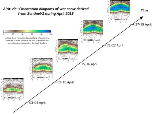
Appendix A. Altitude–Orientation Wet Snow Diagrams

Figure A1. Altitude-orientation diagram from mid-December 2017 to end of March 2018 with the normalized percentage of wet snow-covered pixels by classes of elevation and orientation for Sentinel-1 merged ascending/descending orbits with all slopes. To compute the diagrams, only “useful” pixels are considered for Sentinel-1 (by screening out areas of geometric distortions). The number of “useful” pixels is shown as solid line contours for the ascending orbit and dashed line contours for the descending orbit.
Remotesensing 13 00381 g0a1aRemotesensing 13 00381 g0a1b
Figure A2. Same as Figure A1 but for April to late June 2018.
Remotesensing 13 00381 g0a2aRemotesensing 13 00381 g0a2b

References

  1. Bellaire, S.; Herwijnen, A.V.; Mitterer, C.; Schweizer, J. On forecasting wet-snow avalanche activity using simulated snow cover data. Cold Reg. Sci. Technol. 2017, 144, 28–38. [Google Scholar] [CrossRef]
  2. Jonas, T.; Rixen, C.; Sturm, M.; Stoeckli, V. How alpine plant growth is linked to snow cover and climate variability. J. Geophys. Res. 2008, 113. [Google Scholar] [CrossRef] [Green Version]
  3. Nolin, A.W. Recent advances in remote sensing of seasonal snow. J. Glaciol. 2010, 56, 1141–1150. [Google Scholar] [CrossRef] [Green Version]
  4. Nagler, T.; Rott, H.; Ripper, E.; Bippus, G.; Hetzenecker, M. Advancements for Snowmelt Monitoring by Means of Sentinel-1 SAR. Remote Sens. 2016, 8, 348. [Google Scholar] [CrossRef] [Green Version]
  5. Baghdadi, N.; Gauthier, Y.; Bernier, M. Capability of multitemporal ERS-1 SAR data for wet-snow mapping. Remote Sens. Environ. 1997, 60, 174–186. [Google Scholar] [CrossRef]
  6. Magagi, R.; Bernier, M. Optimal conditions for wet snow detection using RADARSAT SAR data. Remote Sens. Environ. 2003, 84, 221–233. [Google Scholar] [CrossRef]
  7. Nagler, T.; Rott, H. Retrieval of wet snow by means of multitemporal SAR data. IEEE Trans. Geosci. Remote Sens. 2000, 38, 754–765. [Google Scholar] [CrossRef]
  8. Marin, C.; Bertoldi, G.; Premier, V.; Callegari, M.; Brida, C.; Hürkamp, K.; Tschiersch, J.; Zebisch, M.; Notarnicola, C. Use of Sentinel-1 radar observations to evaluate snowmelt dynamics in alpine regions. Cryosphere 2020, 14, 935–956. [Google Scholar] [CrossRef] [Green Version]
  9. Lievens, H.; Demuzere, M.; Marshall, H.P.; Reichle, R.H.; Brucker, L.I.B.; de Rosnay, P.; Dumont, M.; Girotto, M.; Immerzeel, W.W.; Jonas, T.; et al. Snow depth variability in the Northern Hemisphere mountains observed from space. Nat. Commun. 2019, 10, 4629. [Google Scholar] [CrossRef]
  10. Veyssière, G.; Karbou, F.; Morin, S.; Lafaysse, M.; Vionnet, V. Evaluation of Sub-Kilometric Numerical Simulations of C-Band Radar Backscatter over the French Alps against Sentinel-1 Observations. Remote Sens. 2019, 11, 8. [Google Scholar] [CrossRef] [Green Version]
  11. Tsai, Y.L.; Dietz, S.; Oppelt, A.; Kuenzer, N. Remote Sensing of Snow Cover Using Spaceborne SAR: A Review. Remote Sens. 2019, 11, 1456. [Google Scholar] [CrossRef] [Green Version]
  12. Martini, A.; Ferro-Famil, L.; Pottier, E.; Dedieu, J.P. Dry snow discrimination in alpine areas from multi-frequency and multi-temporal SAR data. IEE Proc. Radar Sonar Navig. 2006, 153, 271–278. [Google Scholar] [CrossRef]
  13. Floricioiu, D.; Rott, H. Seasonal and short-term variability of multifrequency, polarimetric radar backscatter of alpine terrain from SIR-C/X- SAR and AIRSAR data. IEEE Trans. Geosci. Remote Sens. 2001, 39, 2634–2648. [Google Scholar] [CrossRef]
  14. Rott, H.; Davis, R.E. Multifrequency and polarimetric SAR observations on alpine glaciers. Ann. Glaciol. 1993, 17, 98–104. [Google Scholar] [CrossRef] [Green Version]
  15. Ulaby, F.; Moore, R.; Fung, A. Microwave dielectric properties of natural earth materials. Microw. Remote Sens. 1986, 3, 2017–2027. [Google Scholar]
  16. Shi, J.; Dozier, J. Inferring Snow Wetness Using C-Band Data from SIR-C’s Polarimetric Synthetic Aperture Radar. IEEE Trans. Geosci. Remote 1995, 33, 905–914. [Google Scholar]
  17. Baghdadi, N.C.L.; Bernier, M. Airborne C-band SAR measurements of wet snow-covered areas. IEEE Trans. Geosci. Remote Sens. 1998, 36, 1977–1981. [Google Scholar] [CrossRef]
  18. Guneriussen, T.; Johnsen, H.; Lauknes, I. RADARSAT, ERS and EMISAR for snow monitoring in mountainous areas. In SAR Workshop: CEOS Committee on Earth Observation Satellites; European Space Agency: Paris, France, 2000; Volume 450, p. 11. [Google Scholar]
  19. Besic, N.; Vasile, G.; Dedieu, J.P.; Chanussot, J.; Stankovic, S. Stochastic approach in wet snow detection using multitemporal SAR data. IEEE Geosci. Remote Sens. Lett. 2015, 12, 244–248. [Google Scholar] [CrossRef] [Green Version]
  20. Haefner, H.; Piesbergen, J. High alpine snow cover monitoring using ERS-1 SAR and Landsat TM data. IAHS Publ.-Ser. Proc. Rep. Intern. Assoc. Hydrol. Sci. 1997, 242, 113–118. [Google Scholar]
  21. Solberg, R.; Amlien, J.; Koren, H.; Eikvil, L.; Malnes, E.; Storvold, R. Multi-sensor and time-series approaches for monitoring of snow parameters. In Proceedings of the Geoscience and Remote Sensing Symposium, 2004. IGARSS’04, Anchorage, AK, USA, 20–24 September 2004; Volume 3, pp. 1661–1666. [Google Scholar]
  22. Goetz, D. Bilan Nivo-Météorologique De L’hiver 2017–2018. Revue de L’ANENA. 2018. Available online: https://www.anena.org/5042-la-revue-n-a.htm (accessed on 1 March 2018).
  23. Stoffel, M.; Corona, C. Future winters glimpsed in the Alps. Nat. Geosci. 2018, 11, 458–460. [Google Scholar] [CrossRef]
  24. Kropatsch, W.G.; Strobl, D. The generation of SAR layover and shadow maps from digital elevation models. IEEE Trans. Geosci. Remote Sens. 1990, 28, 98–107. [Google Scholar] [CrossRef]
  25. Gelautz, M.; Frick, H.; Raggam, J.; Burgstaller, J.; Leberl, F. SAR image simulation and analysis of alpine terrain. ISPRS J. Photogramm. Remote Sens. 1998, 53, 17–38. [Google Scholar] [CrossRef]
  26. Frost, V.S.; Shanmugan, K.S.; Stiles, J.A.; Holtzman, J.C. A Model for Radar Images and Its Application to Adaptive Digital Filtering of Multiplicative Noise. IEEE Trans. Pattern Anal. Mach. Intell. 1982, 4, 157–166. [Google Scholar] [CrossRef] [PubMed]
  27. Small, D. Flattening gamma: Radiometric terrain correction for SAR imagery. IEEE Trans. Geosci. Remote Sens. 2011, 49, 3081–3093. [Google Scholar] [CrossRef]
  28. Wang, P.; Ma, Q.; Wang, J.; Hong, W.; Li, Y.; Chen, Z. An Improved SAR Radiometric Terrain Correction Method and its Application in Polarimetric SAR Terrain Effect Reduction. Prog. Electromagn. Res. B 2013, 54, 107–128. [Google Scholar] [CrossRef] [Green Version]
  29. Gascoin, S.; Grizonnet, M.; Bouchet, M.; Salgues, G.; Hagolle, O. Theia Snow collection: High-resolution operational snow cover maps from Sentinel-2 and Landsat-8 data. Earth Syst. Sci. Data 2019, 11, 492–514. [Google Scholar] [CrossRef] [Green Version]
  30. Techel, F.; Pielmeier, C. Point Observations of liquid water content in natural snow—Investigating methodical, spatial and temporal aspects. Cryosphere Discuss. 2010, 4, 1967–2011. [Google Scholar] [CrossRef]
  31. Wever, N.; Jonas, T.; Fierz, C.; Lehning, M. Model simulations of the modulating effect of the snow cover in a rain-on-snow event. Hydrol. Earth Syst. Sci. 2014, 18, 4657–4669. [Google Scholar] [CrossRef] [Green Version]
  32. Heilig, A.; Mitterer, C.; Schmid, L.; Wever, N.; Schweizer, J.; Marshall, H.P.; Eisen, O. Seasonal and diurnal cycles of liquid water in snow—Measurements and modeling. J. Geophys. Res. Earth Surf. 2015, 120, 2139–2154. [Google Scholar] [CrossRef] [Green Version]
  33. Brun, E. Investigation on wet-snow metamorphism in respect of liquid-water content. Ann. Glaciol. 1989, 13, 22–26. [Google Scholar] [CrossRef] [Green Version]
  34. Waldner, P.; Schneebeli, M.; Schultze-Zimmermann, U.; Flühler, H. Effect of snow structure on water flow and solute transport. Hydrol. Process. 2004, 18, 1271–1290. [Google Scholar] [CrossRef]
  35. Baghdadi, N.; Gauthier, Y.; Bernier, M.; Fortin, J.P. Potential and Limitations of RADARSAT SAR Data for Wet Snow Monitoring. IEEE Trans. Geosci. Remote Sens. 2000, 38, 316–320. [Google Scholar] [CrossRef]
  36. Koskinen, J.; Pulliainen, J.; Hallikainen, M. The use of ERS-1 SAR data in snow melt monitoring. IEEE Trans. Geosci. Remote Sens. 1997, 35, 601–610. [Google Scholar] [CrossRef]
  37. Luojus, K.; Pulliainen, J.; Metsamaki, S.; Hallikainen, M. Snow-Covered Area Estimation Using Satellite Radar Wide-Swath Images. IEEE Trans. Geosci. Remote Sens. 2007, 45, 978–989. [Google Scholar] [CrossRef]
  38. Quegan, S.; Toan, T.L.; Yu, J.J.; Ribbes, F.; Floury, N. Multi-temporal ERS SAR analysis applied to forest mapping. IEEE Trans. Geosci. Remote Sens. 2000, 38, 741–753. [Google Scholar] [CrossRef]
  39. Le, T.T.; Atto, A.; Trouvé, E.; Nicolas, J.M. Adaptive Multitemporal SAR Image Filtering Based on the Change Detection Matrix. IEEE Geosci. Remote Sens. Lett. 2014, 11, 1826–1830. [Google Scholar]
  40. Karbou, F.; James, G.; Durand, P.; Atto, A. Thresholds and distances to better detect wet snow over mountains with Sentinel-1 SAR image time series. In ISTE-WILEY Science- Change Detection and Image Time-Series Analysis, ISTE-WILEY; 2021; Chapter 5; in prep. [Google Scholar]
  41. Malnes, E.; Guneriussen, T. Mapping of snow covered area with Radarsat in Norway. In Proceedings of the IEEE International Geoscience and Remote Sensing Symposium (IGARSS’2002), Toronto, ON, Canada, 24–28 June 2002. [Google Scholar]
  42. Longepe, N.; Allain, S.; Ferro-Famil, L.; Pottier, E.; Durand, Y. Snowpack Characterization in Mountainous Regions Using C-Band SAR Data and a Meteorological Model. IEEE Trans. Geosci. Remote Sens. 2009, 47, 406–418. [Google Scholar] [CrossRef]
  43. Rondeau-Genesse, G.; Trudel, M.; Leconte, R. Monitoring snow wetness in an Alpine Basin using combined C-band SAR and MODIS data. Remote Sens. Environ. 2016, 183, 304–317. [Google Scholar] [CrossRef]
  44. Starovoitov, V.; Samal, D. Experimental study of color image similarity. Mach. Graph. Vis. 1998, 11, 455–462. [Google Scholar]
  45. Di Gesu, V.; Starovoitov, V. Distance-based functionsfor image comparison. Pattern Recognit. Lett. 1999, 20, 207–214. [Google Scholar] [CrossRef]
  46. Zamperoni, P.; Starovoitov, V. On measures of dissimilarity between arbitrary gray-scale images. Int. J. Shape Model. 1996, 2, 189–213. [Google Scholar] [CrossRef]
  47. Kumar, V.; Venkataraman, G. SAR interferometric coherence analysis for snow cover mapping in the western Himalayan region. Int. J. Digit. Earth 2011, 4, 78–90. [Google Scholar] [CrossRef]
  48. Tsai, Y.L.; Dietz, S.; Oppelt, A.; Kuenzer, N. Wet and Dry Snow Detection Using Sentinel-1 SAR Data for Mountainous Areas with a Machine Learning Technique. Remote Sens. 2019, 11, 895. [Google Scholar] [CrossRef] [Green Version]
Figure 1. Location of the study area and surface types from the CORINE Land Cover products. The spatial coverage of Sentinel-1 relative orbits 139 and 161 is shown in the location map.
Remotesensing 13 00381 g001
Figure 2. Wet snow cover extent derived from Sentinel-1 descending/ascending images of 27/28 April 2018 and 20/21 June 2018. Background: IGN Digital elevations.
Remotesensing 13 00381 g002
Figure 3. Snow cover extent derived from Sentinel-2 image of 25 April 2018 and 19 June 2018. Background: IGN Digital elevations.
Remotesensing 13 00381 g003
Figure 4. Shadow/layover/Foreshortening pixels for SAR Ascending and Descending orbits.
Remotesensing 13 00381 g004
Figure 5. Altitude–Orientation diagram with the normalized percentage of wet snow pixels by classes of elevation and orientation for Sentinel-1 (left: ascending, right: descending) for 27–28 April 2018. (Top): Situations with all slopes, (middle): moderate slopes (lower than 20 deg), and (bottom): high slopes. The number of used Sentinel-1 pixels is shown in solid line contours for the ascending orbit and dashed line contours for the descending orbit.
Remotesensing 13 00381 g005
Figure 6. Altitude–Orientation diagram which shows the normalized percentage of snow (wet snow) pixels by classes of elevation and orientation for Sentinel-2 (top, 25 April and 19 June) and Sentinel-1 (bottom, 27–28 April and 20–21 June). Cloudy pixels are screened for Sentinel-2, the number of Sentinel-2 snow pixels is shown in solid line contours. The number of used Sentinel-1 pixels is shown in solid line contours for the ascending orbit and dashed line contours for the descending orbit.
Remotesensing 13 00381 g006
Figure 7. Altitude–Time diagram with the normalized percentage of wet snow-covered pixels by classes of elevation and time for all Sentinel-1 ascending/descending images. Results are given for northern orientations and for moderate slope pixels (lower than 20 degrees).
Remotesensing 13 00381 g007
Figure 8. Same as Figure 7 but for southern orientations.
Remotesensing 13 00381 g008
Table 1. SAR scenes from Sentinel-1 relative orbits A161 (ascending, afternoon) and D139 (descending, early morning) used in this study as well as Sentinel-2 snow products used in this study. Key meteorological and snowpack parameters are also reported: meteorological event; expert elevations of the snow–rain line and continuous snowline (northern and southern orientation); highlights related to the satellites retrievals: presence of clouds and Snowfall reaching Low Altitudes (SLA) for Sentinel-2; origin of wet snow for Sentinel-1: Rain-On-Snow event (ROSE), melt event (ME). Snowpack accumulation period from mid-December 2017 to end of March 2018.
DateSatelliteRelative OrbitMeteorological EventSnow-Rain Line ElevationSnowlines North/SouthHighlight
24 August 2017Sentinel-1D139
25 August 2017Sentinel-1A161
10–11 December 2017Ana storm500 to 2200 m1200 m/1400 mROSE
16 December 2017Sentinel-1D139Snowfall600 to 400 m1000 m/1000 mSLA
17 December 2017Sentinel-1A161
22 December 2017Sentinel-1D139 1000 m/1000 m
23 December 2017Sentinel-1A161
28 December 2017Sentinel-1D139Snowfall1000 to 200 m1000 m/1000 mSLA
29 December 2017Sentinel-1A161Snowfall600 m SLA
3 January 2018Sentinel-1D139Eleanor1500 to 2000 m ROSE
4 January 2018Sentinel-1A161storm2200 m ROSE
5 January 2018Sentinel-2 1000 m/1300 m
9 January 2018Sentinel-1D139Retour d’Est1800 to 1400 m ROSE
10 January 2018Sentinel-1A161
15 January 2018Sentinel-1D139
15 January 2018Sentinel-2 1000 m/1400 mCloudy
16 January 2018Sentinel-1A161Snowfall700 to 1300 m
21 January 2018Sentinel-1D139Heavy snowfall1000 to 1400 mm
22 January 2018Sentinel-1A161Heavy snowfall2000 m ROSE
25 January 2018Sentinel-2 1000 m/1100 mCloudy
27 January 2018Sentinel-1D139Snowfall1000 m
28 January 2018Sentinel-1A161 1000 m/1200 m
30 January 2018Sentinel-2 1000 m/1200 mSea of clouds
2 February 2018Sentinel-1D139
3 February 2018Sentinel-1A161
4 February 2018Sentinel-2 1000 m/1200 mCloudy
8 February 2018Sentinel-1D139
9 February 2018Sentinel-1A161
9 February 2018Sentinel-2 1000 m/1300 m
14 February 2018Sentinel-1D139
14 February 2018Sentinel-2 1000 m/1000 m
15 February 2018Sentinel-1A161Snowfall1800 to 2300 m ROSE
19 February 2018Sentinel-2 1100 m/1200 mCloudy
20 February 2018Sentinel-1D139
21 February 2018Sentinel-1A161
24 February 2018Sentinel-2 1100 m/1300 mCloudy
26 February 2018Sentinel-1D139 Very cold
27 February 2018Sentinel-1A161 Very cold
4 March 2018Sentinel-1D139
5 March 2018Sentinel-1A161
10 March 2018Sentinel-1D139Snowfall2400 m ROSE
11 March 2018Sentinel-1A161Snowfall2500 to 1900 m ROSE
21 March 2018Sentinel-2 1100 m/1300 mCloudy
22 March 2018Sentinel-1D139
23 March 2018Sentinel-1A161
26 March 2018Sentinel-2 1200 m/1500 mCloudy
28 March 2018Sentinel-1D139Snowfall1600 to 18,000 m
29 March 2018Sentinel-1A161Snowfall1800 to 16,000 m
31 March 2018Sentinel-2Heavy snowfall1100 m1100 m/1300 mSLA for the time
Table 2. Same as Table 1 for the 2018 melt season, from early April to mid-June 2018.
DateSatelliteRelative OrbitMeteorological EventSnow-Rain Line ElevationSnowlines North/SouthHighlight
2 April 2018 1000 m/1000 mOnset of the melt season
3 April 2018Sentinel-1D139 1000 m/1000 mME
4 April 2018Sentinel-1A161 1000 m/1200 mME
5 April 2018Sentinel-2 1200 m/1500 mME Cloudy
9 April 2018Sentinel-1D139 1200 m/1500 mME
10 April 2018Sentinel-1A161Snowfall1200 m1200 m/1400 mSLA for the time
15 April 2018Sentinel-1D139 1400 m/1700 mME
15 April 2018Sentinel-2 1400 m/1700 mME
16 April 2018Sentinel-1A161 1400 m/1700 mME
20 April 2018Sentinel-2 1400 m/1700 mME
21 April 2018Sentinel-1D139 1500 m/1800 mME
22 April 2018Sentinel-1A161 1600 m/1900 mME
25 April 2018Sentinel-2 1600 m/2000 mME
27 April 2018Sentinel-1D139 1700 m/2000 mME
28 April 2018Sentinel-1A161 1700 m/2000 mME
3 May 2018Sentinel-1D139Retour d’Est2800 m1900 m/2200 mSmall amount
4 May 2018Sentinel-1A161Retour d’Est2500 m1900 m/2300 mSmall amount
5 May 2018Sentinel-2 1900 m/2300 mCloudy
9 May 2018Sentinel-1D139 1700 m/2000 mME
10 May 2018Sentinel-1A161Snowfall2600 m1700 m/2000 mMS/ ROSE
13 May 2018Snowfall1500 m1500 m/2300 mSLA for the time
15 May 2018Sentinel-1D139Snowfall2000 to 2400 m1500 m/2000 mROSE
15 May 2018Sentinel-2Snowfall2000 to 2400 m1500 m/2000 mCloudy
16 May 2018Sentinel-1A161 1900 m/2300 mME
20 May 2018Sentinel-2 2000 m/2300 mStormy
21 May 2018Sentinel-1D139Instable2600 m2000 m/2300 mME
22 May 2018Sentinel-1A161Instable2800 m2000 m/2300 mME
25 May 2018Sentinel-2 2000 m/2300 mPartly cloudy
27 May 2018Sentinel-1D139Instable3400 m2000 m/2400 mME
28 May 2018Sentinel-1A161Instable3200 m2000 m/2500 mME
2 June 2018Sentinel-1D139Instable3500 m2000 m/2600 mME
3 June 2018Sentinel-1A161Instable3400 m2100 m/2600 mME
8 June 2018Sentinel-1D139Instable 2200 m/2600 mME
9 June 2018Sentinel-2Instable 2200 m/2600 mCloudy
9 June 2018Sentinel-1A161Instable 2200 m/2600 mME
14 June 2018Sentinel-1D139 //ME
14 June 2018Sentinel-2 //ME Cloudy
15 June 2018Sentinel-1A161 //ME
19 June 2018Sentinel-2 -ME
20 June 2018Sentinel-1D139 -ME
21 June 2018Sentinel-1A161 -ME
26 June 2018Sentinel-1D139 -ME
27 June 2018Sentinel-1A161 -ME
Table 3. Percentage of the surface covered by wet snow using images of the descending orbit (left) and the ascending orbit (right). The results are given using an average summer image as a reference and using a reference image taken in early September. 100% means that the entire study area is covered by wet snow.
DateSummerEarly Sep.DateSummerEarly Sep.
28 March 20187.16.929 March 201821.318.6
3 April 201814.915.44 April 201824.421.7
9 April 201827.426.310 April 201834.230.4
15 April 201824.924.516 April 201843.040.6
21 April 201832.031.522 April 201839.336.6
27 April 201835.735.728 April 201838.636.4
3 May 201830.930.84 May 201833.230.8
9 May 201832.332.310 May 201833.131.1
15 May 201827.727.716 May 201837.334.2
21 May 201828.528.722 May 201828.426.2
27 May 201819.519.428 May 201820.519.8
2 June 201821.221.23 June 201819.618.9
8 June 201815.715.39 June 201816.014.9
14 June 201816.516.515 June 201815.514.4
20 June 201810.910.821 June 201810.510.0
26 June 201810.711.427 June 20189.99.2
Publisher’s Note: MDPI stays neutral with regard to jurisdictional claims in published maps and institutional affiliations.

