TomoSAR Mapping of 3D Forest Structure: Contributions of L-Band Configurations

Abstract

Synthetic Aperture Radar (SAR) measurements are unique for mapping forest 3D structure and its changes in time. Tomographic SAR (TomoSAR) configurations exploit this potential by reconstructing the 3D radar reflectivity. The frequency of the SAR measurements is one of the main parameters determining the information content of the reconstructed reflectivity in terms of penetration and sensitivity to the individual vegetation elements. This paper attempts to review and characterize the structural information content of L-band TomoSAR reflectivity reconstructions, and their potential to forest structure mapping. First, the challenges in the accurate TomoSAR reflectivity reconstruction of volume scatterers (which are expected to dominate at L-band) and to extract physical structure information from the reconstructed reflectivity is addressed. Then, the L-band penetration capability is directly evaluated by means of the estimation performance of the sub-canopy ground topography. The information content of the reconstructed reflectivity is then evaluated in terms of complementary structure indices. Finally, the dependency of the TomoSAR reconstruction and of its structural information to both the TomoSAR acquisition geometry and the temporal change of the reflectivity that may occur in the time between the TomoSAR measurements in repeat-pass or bistatic configurations is evaluated. The analysis is supported by experimental results obtained by processing airborne acquisitions performed over temperate forest sites close to the city of Traunstein in the south of Germany.

1. Introduction

Forest (canopy) structure is commonly defined as “the organization in space and time, including the position, extent, quantity, type and connectivity, of the aboveground components of vegetation” [1,2,3,4,5]. Mapping forest structure is critical for understanding the history, function and future of forest ecosystems. Indeed, forest structure expresses forest state, functionality, biodiversity and evolution, and is an indicator of the successional stage and development as well as sustainability and habitability [6,7,8]. Due to this, it is an important parameter for assessing forest productivity, biomass and biodiversity [9,10,11,12]. Finally, the knowledge of structure evolution in time (due to anthropogenic or natural disturbance, regeneration, growth, etc.) supports the modelling of the function and development of forest ecosystems and the development of accurate and robust forest biomass estimators [13].

Remote sensing techniques have the potential to map the 3D distribution of vegetation compartments and of their changes at large scales with spatial and temporal continuity. Today, only lidar and Synthetic Aperture Radar (SAR) can provide 3D information with metric resolution and repeatedly in time and contribute to the observation and quantitative characterization of forest structure at large scales [14,15]. While lidar configurations allow a more or less dense sampling of accurate (vertical) structure measurements, SAR configurations realize imaging with wide swath widths enabling continuous global scale coverage with high spatial (e.g., on the order of 10 m) and temporal (e.g., on the order of weekly) resolutions [15].

The relative importance of the different tree and stand components (e.g., leaves, branches, trunks) in SAR measurements depends on the wavelength and polarization employed, and on the geometric (e.g., size) and dielectric properties of these components defined by the amount and distribution of water [14,15]. With increasing wavelength, SAR pulses penetrate more and more into and through the forest canopy and interact with forest elements located at different heights within the forest volume as well as with the underlying ground. However, a single SAR image does not allow a reconstruction of the 3D distribution of scatterers within the illuminated volume. For this a set of SAR images acquired under (slightly) different incidence angles is required in the context of interferometric (InSAR) and/or tomographic SAR (TomoSAR) measurements [14,15]. The reconstruction of 3D reflectivity is today understood and established and has been demonstrated in several (airborne and spaceborne) experiments [15,16,17,18,19,20,21,22]. However, the interpretation of the reconstructed 3D reflectivity in terms of physical 3D structure is still in a rather early stage.

Across the electromagnetic spectrum, L-band (with a wavelength of about 24 cm) is more versatile for forest structure applications than other frequencies as it provides a reasonable compromise between sensitivity to structurally relevant canopy scattering components and the capability to penetrate through the canopy until the ground ensuring the “visibility” of the whole forest volume in a wide range of forest types and conditions. At the same time, the higher temporal stability of the scatterers at L-band (when compared to scatterers at higher frequencies) leads to lower temporal decorrelations in repeat-pass configurations. Finally, also with respect of the actual bandwidth allocations imposed by the International Telecommunication Union (ITU) regulations that rule the bandwidth available for Earth Observation (EO) space borne realizations at the different frequencies, L-band appears as the optimal compromise between possible spatial (range) resolution and interferometric/tomographic performance.

The general inversion problem behind any TomoSAR estimation is defined in Section 2, discussing the challenges in the TomoSAR estimation of 3D reflectivity at L-band. Section 3 addresses methodological aspects in the extraction of structure information from the TomoSAR reflectivity, with particular focus on the role of reflectivity maxima (e.g., peaks). A critical point is the distinction of reflectivity peaks associated to scattering contributions from ones induced by focusing ambiguities and artifacts. The contribution of L-band TomoSAR reflectivity reconstructions for the (quantitative) characterization of 3D forest structure is reviewed and further assessed. For this, the structure framework recently proposed in [23,24] in which the distribution of reflectivity peaks is used to derive indices describing the (physical) structural complexity in the horizontal and vertical directions is presented. After describing the considered test sites and data sets in Section 4, Section 5, Section 6 and Section 7 report and discuss experimental results with respect to:

• Penetration and information content (Section 5)–First, the ability of L-band to penetrate into and through the canopy down to the ground is assessed directly in terms of both the ground-to-volume power ratio and the estimation performance for the location of the underlying ground. Second, the capability in deriving physical forest structure indices from L-band TomoSAR reflectivity is discussed within the chosen structure framework. In this, the understanding of the role of the availability of multiple polarization channels is of particular importance.
• TomoSAR imaging geometry (Section 6)–Conditioned to the (TomoSAR) reconstruction algorithm, different TomoSAR geometries in terms of the distribution of tracks/orbits in the direction orthogonal to the line of sight, and the number of images lead to different vertical resolutions and quality (e.g., in terms of ambiguities) for the reconstructed reflectivity. The imaging geometry depends primarily on flight/orbital constraints, but also changes across a scene with the incidence angle variation from near- to far-range. The impact of such changes on the spatial gradients the retrieved structure descriptors is evaluated.
• Technical implementation (Section 7)—At present, there is no configuration that allow a simultaneous acquisition of all TomoSAR images. As a consequence, any configuration is affected by changes of the 3D reflectivity in time. While these changes can be neglected in typical L-band airborne acquisitions where short repeat-pass times are possible, they become relevant in space borne ones. For this, conventional repeat-pass and bistatic TomoSAR implementations are compared in terms of their ability to retrieve physical structure information in presence of temporal reflectivity changes.

Finally, the conclusions are drawn in Section 8. The analysis is supported by experimental results achieved in the framework of recent airborne SAR (DLR’s F-SAR platform) campaigns over two forest sites close to the city of Traunstein in south Germany.

2. SAR Tomography for the Estimation of the Vertical Reflectivity Profiles

2.1. The TomoSAR Inversion Problem

In monostatic TomoSAR acquisitions $K$ single-look complex (SLC) images are collected with slightly different incidence angles in $N_P$ polarimetric channels along displaced tracks/orbits. For a fixed polarization $\mathsf{\omega }$ and range-azimuth coordinate, after coregistration, compensation of the range dependent phase component (e.g., flat-Earth compensation), phase calibration and spectral shift filtering [25], the complex amplitudes of the different images are collected in the $K$—dimensional vector $\mathrm{y}\left(\mathsf{\omega }\right)$. The associated TomoSAR covariance matrix is $\mathrm{R}\left(\mathsf{\omega }\right):=E\left\{\mathrm{y}\left(\mathsf{\omega }\right){\mathrm{y}}^{\mathrm{H}}\left(\mathsf{\omega }\right)\right\}$, where $E\left\{·\right\}$ and ${\left(·\right)}^H$ indicate the statistical expectation and the Hermitian operators, respectively. The generic $\left(m,n\right)—$th element of $\mathrm{R}\left(\mathsf{\omega }\right)$ can be written in terms of the underlying vertical reflectivity profile $F\left(z, \mathsf{\omega }\right)$ as [14,16]:

$${\left[\mathrm{R}\left(\mathsf{\omega }\right)\right]}_{m,n}={{\displaystyle \int }}^{ }F\left(z, \mathsf{\omega }\right)e^{j\left({\kappa }_{Z,m}-{\kappa }_{Z,n}\right)z}dz.$$

(1)

where ${\kappa }_{Z,k}$ is the vertical wavenumber [25,26] associated to the $k—$th image.

The TomoSAR inversion problem concerns the estimation of $F\left(z, \mathsf{\omega }\right)$ by means of the inversion of the Fourier relationship in Equation (1) applied to an estimate of $\mathrm{R}\left(\mathsf{\omega }\right)$ in a multilook cell consisting of $N$ independent samples (e.g., looks). The maximum available wavenumber determines the Rayleigh vertical resolution of the reconstruction [14,16,26]:

$${\delta }_Z=\frac{2\pi }{\max \left({\left\{{\kappa }_{Z,k}\right\}}_{k=1}^K\right)}.$$

(2)

2.2. Challenges of TomoSAR Imaging of Forest Volumes at L-Band

Due to penetration, L-band (back-)scattering occurs at multiple heights within the volume, and it is reasonable to assume continuous and extended vertical reflectivity profiles. For this reason, the TomoSAR inversion problem is typically underdetermined as the number of the available images $K$ is lower than the number of profile amplitudes required to be estimated for an appropriate characterization of $F\left(z, \mathsf{\omega }\right)$.

As a rule of thumb, for Rayleigh vertical resolutions in the order of 10 m and not too irregularly distributed wavenumbers, non-parametric spectral estimators are a reasonable choice in terms of final reconstruction performance [26]. The Capon spectral estimator improves the vertical resolution and the sidelobe attenuation of a direct Fourier spectral estimator [26,27,28,29], and provides a data-adaptive estimate $F_C\left(z, \mathsf{\omega }\right)$:

$$F_C\left(z, \mathsf{\omega }\right)={\mathrm{h}}^H\left(z, \mathsf{\omega }\right)\mathrm{R}\left(\mathsf{\omega }\right)\mathrm{h}\left(z, \mathsf{\omega }\right)\hspace{1em}\mathrm{with}\hspace{1em}\mathrm{h}\left(\mathrm{z}, \mathsf{\omega }\right)=\frac{\mathrm{R}{\left(\mathsf{\omega }\right)}^{-1} \mathrm{a}\left(z\right)}{{\mathrm{a}}^H\left(z\right)\mathrm{R}{\left(\mathsf{\omega }\right)}^{-1} \mathrm{a}\left(z\right)}$$

(3)

$\mathrm{h}\left(\mathrm{z}, \mathsf{\omega }\right)$ is a filter that minimizes for each $z$ the interference of the contributions coming from other heights by adaptively placing proper nulls. The $K—$dimensional steering vector $\mathrm{a}\left(z\right)$ contains the height ($z$)–dependent phase differences of all images with respect to the reference one. Its $k—$th element is ${\left[\mathrm{a}\left(z\right)\right]}_k=e^{j{\kappa }_{Z,k}z}$. Even though widely employed, the tomographic formulation of (3) does not match to forest volumes by design [26,28,29]. The expected resolution and sidelobe attenuation improvements refer to a (deterministic) Dirac-$\delta$ approximation of the scattering contribution at each height. However, in a forest volume every single scattering contribution cannot be considered isolated from the others. As a consequence, in order to deal with the underdetermination of the inversion, the Capon optimization provides the maximum reflectivity value among the possible ones, introducing biases in the radiometric reconstruction of the (forest) volume scattering contributions [30]. This is independent of the track distribution, meaning that an improvement in the Rayleigh vertical resolution is in general not sufficient to improve the radiometric accuracy. Additional non-idealities like an inaccurate knowledge of $\mathrm{R}\left(\mathsf{\omega }\right)$ (in terms of a biased estimation) and/or $\mathrm{a}\left(z\right)$ (due to residual track positioning errors or atmospheric propagation) results into additional radiometric inaccuracies, that can finally end up even in underestimating stronger contributions (self-cancellation) [27,28]. However, they can be mitigated by diagonally loading $\mathrm{R}\left(\mathsf{\omega }\right)$ in $\mathrm{h}\left(\mathrm{z}, \mathsf{\omega }\right)$, thus reducing the adaptivity and tending in the limit to a Fourier estimate [24].

There are alternative approaches to better account for the presence of volumes. The first one relies on a parametric description (e.g., modeling) of the reflectivity function. Such an approach is used for instance for the generalized Capon formulations in [31] and [32], which are also related to more general covariance matching approaches [29]. The second approach does not model the reflectivity profile but constrains the solution (sub-)space of the TomoSAR inversion. This is the case of the Polarization Coherence Tomography [33] and Compressive Sensing [34,35,36] approaches. The physical significance of the model parameters and of the constrained solution space directly affect the physical significance and the accuracy of the final reflectivity estimates. To date there are no established full electromagnetic models nor appropriate (sub-)spaces fully supporting an accurate TomoSAR profile inversion especially at L-band.

3. Physical Information Extraction from the Reflectivity Profiles: Distribution of Peaks

The potentials and limitations of TomoSAR reconstructions are today understood and well assessed experimentally [26]. However, the interpretation of reflectivity profiles in terms of 3D physical structure attributes is not as established at any of the frequencies and in particular not at L-band. Two aspects make this interpretation challenging:

• At a fixed wavelength, the relative scattering contribution of the different vegetation elements with respect to each other depends on the viewing geometry (e.g., the incidence angle), the polarization, but also on their dielectric properties, which are relevant at L-band [37]. There are not appropriate electromagnetic models able to describe these dependencies accurately enough to provide a transfer function between the 3D distribution of vegetation elements and 3D reflectivity. Additionally, the limited resolution of conventional SAR systems does not allow to distinguish single trees, preventing a direct correspondence between TomoSAR reflectivity and conventional (single-tree based) structural descriptors established in forestry and ecology.
• The TomoSAR acquisition configuration and profile reconstruction algorithm(s) concur to determine both (i) the resolution at which the profile peaks corresponding to scattering contributions (i.e., the scatterer mainlobes) can be distinguished from each other in height, and (ii) the level of the sidelobes of each of them. Weaker scattering contributions are particularly penalized as their mainlobe can be confused with, or even masked by, the sidelobes of stronger contributions. The regularity (e.g., distribution) of the wavenumbers plays a critical role, but also the temporal distribution of the acquisitions compared to the changes of reflectivity [26] is significant.

Recently, there have been several attempts to use TomoSAR profiles for structure characterization [23,24,38] and biomass estimation [39,40,41]. Alternatively to the approaches using the full reflectivity information, the distribution of profiles peaks has been explored as well after detecting the meaningful ones. For instance, within a height interval of interest, the meaningful peaks at the lowest and highest heights can be used to extract ground topography [22,42] and top height [43], respectively. Moreover, it has been shown by models and experiments that the 3D distribution of the identified meaningful peaks reflects the variability of the vegetation elements within a stand [18,44,45,46], supporting the assumption of their physical significance. In this framework, the ability to identify the meaningful peaks corresponding to “true” scattering contributions is critical and depends on the TomoSAR reconstruction algorithm as well as on the acquisition configuration.

3.1. Coherence Matrix Model

Without losing generality, the estimation of a normalized $F\left(z,\mathsf{\omega }\right)$ from the inteferometric complex coherence matrix $\mathsf{\Gamma }\left(\mathsf{\omega }\right)$ associated to $\mathrm{R}\left(\mathsf{\omega }\right)$ is considered.

$$\mathsf{\Gamma }\left(\mathsf{\omega }\right)={\mathrm{W}}^{-1/2}\mathrm{R}\left(\mathsf{\omega }\right){\mathrm{W}}^{-1/2},$$

(4)

where $\mathrm{W}$ is a diagonal matrix with ${\left[\mathrm{W}\right]}_{k,k}={\left[\mathrm{R}\left(\mathsf{\omega }\right)\right]}_{k,k}$. As coherence values are normalized by the SLC intensity, the methodologies and analyses reported in the following are independent of radiometric correction factors applied e.g., to reduce modulations of the backscattered power induced by slopes.

For $\mathsf{\Gamma }\left(\mathsf{\omega }\right)$a number of model assumptions are considered. First of all, the received signal is modelled as the sum of the backscattered signal with power $P_S\left(\mathsf{\omega }\right)$ and receiver white noise with power $P_N\left(\mathsf{\omega }\right)$. As a consequence:

$$\mathrm{R}\left(\mathsf{\omega }\right)=P_S\left(\mathsf{\omega }\right){\mathsf{\Gamma }}_S\left(\mathsf{\omega }\right)+P_N\left(\mathsf{\omega }\right)\mathrm{I} \Rightarrow \mathsf{\Gamma }\left(\mathsf{\omega }\right)=\frac{SNR\left(\mathsf{\omega }\right)}{SNR\left(\mathsf{\omega }\right)+1}{\mathsf{\Gamma }}_S\left(\mathsf{\omega }\right)+\frac{1}{SNR\left(\mathsf{\omega }\right)+1}\mathrm{I},$$

(5)

where $SNR\left(\mathsf{\omega }\right)=P_S\left(\mathsf{\omega }\right)/P_N\left(\mathsf{\omega }\right)$, and I denotes the identity matrix. In the absence of temporal decorrelation (i.e., no reflectivity changes during the TomoSAR acquisition time), the signal coherence matrix ${\mathsf{\Gamma }}_S\left(\mathsf{\omega }\right)$ can in turn be written as the sum of a ground and a volume contribution as for example addressed by the so called Random-Volume-over-Ground (RVoG) model [47,48]:

$${\mathsf{\Gamma }}_S\left(\mathsf{\omega }\right)=\frac{\mu \left(\mathsf{\omega }\right)}{\mu \left(\mathsf{\omega }\right)+1}{\mathsf{\Gamma }}_G+\frac{1}{\mu \left(\mathsf{\omega }\right)+1}{\mathsf{\Gamma }}_V,$$

(6)

where $\mu \left(\mathsf{\omega }\right)$ is the ground-to-volume amplitude ratio, and ${\mathsf{\Gamma }}_G=\mathrm{a}\left(z_G\right){\mathrm{a}}^H\left(z_G\right)$ with $z_G$ the ground height. The RVoG model assumes that the volume-only reflectivity is but for a scaling factor the same across all polarimetric channels, and that the ground reflectivity is described by a Dirac-$\delta$ function [47,48]. Equations (5) and (6) can be put together in a compact form as:

$$\mathsf{\Gamma }\left(\mathsf{\omega }\right)=\alpha \left[\beta \mathrm{a}\left(z_G\right){\mathrm{a}}^H\left(z_G\right)+\left(1-\beta \right){\mathsf{\Gamma }}_V\right]+\left(1-\alpha \right) \mathrm{I}$$

(7)

with $\alpha =SNR\left(\mathsf{\omega }\right)/\left[1+SNR\left(\mathsf{\omega }\right)\right]$ and $\beta =\mu \left(\mathsf{\omega }\right)/\left[1+\mu \left(\mathsf{\omega }\right)\right]$.

Equation (7) is formally valid also in the presence of residual phase calibration errors. Let $\mathsf{\phi }$ be a $K—$dimensional vector containing the phase errors at the different images. Usually,$\mathsf{\phi }$ is assumed to be a zero-mean Gaussian distributed vector with covariance matrix ${\sigma }_{\phi }^2 \mathrm{I}$ [49,50]. In presence of phase errors, $\mathrm{R}\left(\mathsf{\omega }\right)$ becomes [49,50].

$$\mathrm{R}\left(\mathsf{\omega }\right)=P_S\left(\mathsf{\omega }\right){\mathrm{E}\mathsf{\Gamma }}_S\left(\mathsf{\omega }\right){\mathrm{E}}^H+P_N\left(\mathsf{\omega }\right)\mathrm{I}$$

(8)

in which $\mathrm{E}$ is a diagonal matrix with ${\left[\mathrm{E}\right]}_{k,k}=e^{j{\left[\mathsf{\phi }\right]}_k}$. For a small enough ${\sigma }_{\phi }^2$, the approximation ${\left[\mathrm{E}\right]}_{k,k}\approx 1+j{\left[\mathsf{\phi }\right]}_k$ holds, and it results [49]:

$$\mathrm{R}\left(\mathsf{\omega }\right)\approx P_S\left(\mathsf{\omega }\right){\mathsf{\Gamma }}_S\left(\mathsf{\omega }\right)+P_S\left(\mathsf{\omega }\right){\sigma }_{\phi }^2\mathrm{I}+P_N\left(\mathsf{\omega }\right) \mathrm{I}.$$

(9)

Thus, it is straightforward to see that Equation (7) can be obtained from Equation (9) for $\alpha =SNR\left(\mathsf{\omega }\right)/\left[1+SNR\left(\mathsf{\omega }\right)\left(1+{\sigma }_{\phi }^2\right)\right]$.

3.2. Ground Topography

The hypothesis of a Dirac-$\delta$ ground reflectivity implies that the ground scattering contribution induces at $z_G$ a peak in the reflectivity profile. As a consequence, $z_G$ can be estimated from a TomoSAR profile as the position of the meaningful peak at the lowest height. Meaningful peaks are supposed to exceed an amplitude threshold $T$. The choice of an appropriate value of T for distinguishing the ground peak from the nearby sidelobes is addressed in the following.

If no diagonal loading is applied, the Capon profile estimate can be written in a compact form as:

$$F_C^{-1}\left(z, \mathsf{\omega }\right)=F_{C,VN}^{-1}\left(z\right)-\frac{\alpha \beta {\left|{\mathrm{a}}^H\left(z\right)\mathsf{\Gamma }\left(\mathsf{\omega }\right)\mathrm{a}\left(z_G\right)\right|}^2}{1+\alpha \beta F_{C,VN}^{-1}\left(z_G\right)}$$

(10)

where $F_{C,VN}\left(z\right)$ is the Capon profile associated to the volume-only under the RVoG hypothesis and noise components:

$${\mathsf{\Gamma }}_{VN}=\alpha \left(1-\beta \right){\mathsf{\Gamma }}_V+\left(1-\alpha \right)\mathrm{I}.$$

(11)

Considering only the $z$ range around and below the ground height $z_G$ and neglecting the volume contributions means approximating ${\mathsf{\Gamma }}_{VN}\approx \left(1-\alpha \right)\mathrm{I}$, leading to:

$$F_C^{-1}\left(z\right)\approx \frac{K}{1-\alpha }-\frac{\alpha \beta }{1-\alpha }\frac{K^2\mathrm{PSF}\left(z-z_G\right)}{\left(1-\alpha \right)+\alpha K}$$

(12)

where $\mathrm{PSF}\left(z-z_G\right)={\left|{\mathrm{a}}^H\left(z\right)\mathrm{a}\left(z_G\right)\right|}^2/K^2$ indicates the TomoSAR point spread function centered around $z_G$, and corresponds to the Fourier profile of a point-like scatterer located at $z_G$. Therefore, the TomoSAR PSF determines the position and the amplitudes of the sidelobes of $F_C\left(z, \mathsf{\omega }\right)$ in the selected height interval. For detecting the ground, it is sufficient to set the following threshold:

$$T=\frac{\left(1-\alpha \right)\left[\left(1-\alpha \right)+\alpha K\right]}{K\left(1-\alpha \right)+\alpha K^2-\alpha \beta K^{2}PSL},$$

(13)

corresponding to the highest sidelobe amplitude expressed by the PSL (peak-sidelobe level). The use of the PSL in Equation (13) is appropriate as long as the highest sidelobe is next to the mainlobe in the PSF, as in the reported experiment. Should this not be the case, the amplitude of the PSF sidelobe closest to the mainlobe should be used instead. Complications arise if the volume-only reflectivity is not negligible around the ground height $z_G$. This may introduce a systematic bias in the position of the ground peak if the first derivative of volume-only profiles does not equal zero at $z_G$. At the same time, an optimization of the threshold value can be carried out only by making assumptions on ${\mathsf{\Gamma }}_V$ and/or on the level of the corresponding sidelobes. Finally, there is a minimum ground-to-volume ratio ${\mu }_{min}$ required for the detection of the ground. Assuming now both the noise ($\alpha \to 1$) and the ground estimation bias to be negligible, it results:

$${\mu }_{min}=\frac{T-F_{C,V}\left(z_G\right)}{1-T}$$

(14)

where $T$ is now a generic threshold.

3.3. Horizontal and Vertical Structure Indices

Indices based on the 3D distribution of the identified meaningful peaks between ground and canopy top within a given area on ground (referred as structure window in the following) can be used to interpret TomoSAR profiles in terms of structural heterogeneity in the horizontal and vertical dimensions. Let $\mathcal{P}=\{p_1,p_2,\dots ,p_P\}$ be the ensemble of the $P$ peaks in the structure window (excluding the ground peaks), and $\mathcal{Z}=\left\{z_1,z_2,\dots ,z_M\right\}$the ensemble of the corresponding $M$ unique peak heights. A horizontal structure index $HS$ can be defined as [16,17]:

$$HS:=1-H{S}_0/H{S}_{0, max}$$

(15)

where:

$$H{S}_0:=\frac{n({\mathcal{P}}_{top})}{A}$$

(16)

where $n({\mathcal{P}}_{top})$ is the number of elements of a subset ${\mathcal{P}}_{top}$ of $\mathcal{P}$ constituted by all the peaks with height in the top (vegetation) layer, $A$ is the area of the structure window and $H{S}_{0, max}$ is a (reference) maximum value. The top layer corresponds to the range of heights above $\epsilon ·\max \left(\mathcal{Z}\right)$, where $\epsilon <1$ is a usually empirically defined factor. $H{S}_0$ expresses then the density of peaks in the top layer: the larger the number of peaks, the denser (homogeneous) the stands and $HS$ tends to 0. $HS$ tends to 1 in the opposite case, indicating a sparser (heterogenous) stand. At the same time, a vertical structure index $VS$ can be defined as [23,24]:

$$VS:=V{S}_0/V{S}_{0, max} , V{S}_0=M \mathrm{var}\left\{\mathcal{Z}\right\},$$

(17)

where $\mathrm{var}\left\{\mathcal{Z}\right\}$ is the variance of the peak heights in $\mathcal{Z}$ and $V{S}_{0, max}$ is a reference normalization value. Similarly to $HS$, $VS$ increasing to 1 corresponds to increasing vertical heterogeneity. In [22,24], it has been shown that the indices in Equations (15)–(17) agree in different forest types with equivalent indices estimated from lidar data. Even more, they correlate with equivalent indices used in forestry and ecology derived from field measurements linking space occupation with tree size. In particular, $HS$ correlates with the stand density index (closely related to the basal area) and $VS$ with the standard deviation of the diameter at breast height [24]. The calculation of the structure indices in Equations (15)–(17) presupposes the accurate identification meaningful peaks, also here usually implemented through an amplitude threshold. Different than in the case of ground topography estimation, no reliable a priori assumptions can be made for the volume and a reasonable threshold value can be only empirically set. However, an intrinsic robustness against missed detection and false alarms can actually be expected, as Equations (15)–(17) rely on statistics of ${\mathcal{P}}_{top}$ and $\mathcal{Z}$, and can be further increased by increasing the window area $A$ for a fixed TomoSAR profile resolution. $P$ and $M$ will increase accordingly, and the possible sidelobes included in the selection are expected to play only a secondary role. However, this could limit structure windows to larger values, reducing its significance for heterogenous stands [24].

4. Test Sites and Data Sets

The experimental analyses in the next Sections have been carried out by processing TomoSAR airborne L-band data sets acquired by the DLR’s F-SAR platform over two temperate forest sites located in the proximity of Traunstein in the south of Germany. The location of the two sites is depicted in Figure 1a.

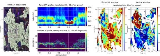
The first site is in a locality called Froschham. The topography is essentially flat around 590 m above sea level, and canopy heights reach 40 m. Management activities aim at transforming even aged monospecific stands into uneven aged mixed species stands. This transition has been captured by the TomoSAR acquisition. Homogenous forest stands dominate the eastern part (appearing in near range and lower azimuth distances in the Pauli RGB composite image in Figure 1b), while the western part (higher azimuth distances and/or far range) is characterized by multi-layered mixed stands and complex stand structure. This clear differentiation extending for several hectares makes this site ideal for investigating the structural information content of L-band TomoSAR profiles, and its sensitivity to the acquisition geometry reported in Section 5 and Section 6. In 2015, an extensive ground measurement campaign took place in a 25 ha plot that has been included in the ForestGEO network [51]. In addition to the extensive ground measurements, in 2016 fine-beam airborne Lidar data were collected over this site and are used in this paper for comparison. The TomoSAR acquisition took place in June 2017. In this experiment, $K=15$ images have been acquired along uniformly distributed tracks with a horizontal displacement between 5 and 70 m at a reference flight height of about 3000 m above mean terrain height. The data set has been processed by a standard repeat-pass interferometric processor, including co-registration, flat-Earth and terrain phase compensation and residual phase calibration [52]. The processed range and azimuth SLC resolutions are 1.3 m and 0.6 m, respectively. The final Rayleigh vertical resolution varies between 3 m in near and 9 m in far range. The acquisition parameters are summarized in

Table 1. Relevant acquisition parameters of the processed data sets.

Test Site	Date	${\mathit{\kappa }}_{\mathit{Z}} (\mathbf{rad}/\mathbf{m}){ }^1$	Resolution (m)
			Vertical 1	Range	Azimuth
Froschham	11 May 2017	0 2, 0.02, 0.09, 0.13, 0.18, 0.24, 0.33, 0.36, 0.42, 0.5, 0.58, 0.65, 0.69, 0.77, 0.83	7.5	1.3	0.6
Traunstein	20 May 2014	0, 0.06, 0.12, 0.18, 0.24	26.1	1.3	0.6
	10 June 2014
	16 June 2014
	28 July 2014
Traunstein Repeat-pass	20 May 2014	0.24	26.1	1.3	0.6
	10 June 2014	0.18
	16 June 2014	0.12
	28 July 2014	0, 0.06
Traunstein Bistatic	20 May 2014	0.24	26.1	1.3	0.6
	10 June 2014	0.18
	16 June 2014	0.12
	28 July 2014	0.06

¹ Values at mid-range after averaging along azimuth; ² ${\kappa }_Z$ = 0 indicates the reference track.

.

The second site is the Traunstein Bürgerwald forest, indicated by the southern polygon in Figure 1a. Through the years, the Traunstein forest is being reconverted from a homogeneous one-age forest to a structurally rich, heterogeneous forest. Most forest stands are complex in terms of tree species richness and heterogeneous stand structures. The topography ranges from 630 to 720 m above sea level and is general flat with localized steep slopes. Forest top heights reach 40 m. The “close-to-nature” silviculture is reflected in five growth stages distributed across the site according to field inventories [53]. Young stands are constituted predominantly by young trees with low density. Density increases in the growing forest stands, which include scattered taller trees above the young shorter ones. Stands in a transition stage are characterized by regrowth of shorter trees below an older and taller vegetation layer. Mature stands are homogenous with a dense top canopy layer. Finally, the so-called “Plenterwald”stands are very heterogeneous in terms of species and ages. The German term “Plenterwald” (selection cutting) indicates forest stands undergoing management procedures aiming at boosting structure heterogeneity in a constant mixture of trees of different species and ages. In 2014, The DLR’s F-SAR system flew four times in more than two months on May 20, June 10, June 16 and July 28 [26]. A Pauli RGB composite image is shown in Figure 1c. Each time the same slightly irregular TomoSAR configuration consisting of 5 tracks displaced in the horizontal direction by up to 25 m was acquired (see Table 1 for additional acquisition parameters). However, deviations from the nominal tracks resulted into more or less significant distortions of the PSF. The largest one occurred on June 10, and the related PSF can locally exhibit sidelobes up to just −4 dB with respect to the main lobe [26]. In order to minimize the TomoSAR performance across the four sets, the corresponding data vectors have been interpolated to a common uniform wavenumber distribution using the interpolator in [54]. The interpolation process was implemented exactly as discussed in [55] and was constrained by the individual volume heights fixed here according to a fine-beam lidar acquisition carried out in 2012. Each data set was collected in less than 1 h and given the calm wind conditions temporal decorrelation between the individual tracks is assumed negligible. As the four data sets span a time interval of two months, they are suitable to evaluate different TomoSAR implementations in terms of the provided robustness of structure indices to changes of the vertical reflectivity profiles induced by seasonality in Section 7. The weather stations in Nilling and Schönharting located within a 20 km radius from the Bürgerwald reported very similar weather conditions for all four campaign days [26].

5. Structural Information Content of L-Band TomoSAR Profiles

5.1. Reference Lidar Structure Indices

The lidar data, e.g., the ground topography (digital terrain model, DTM) and canopy height (canopy height model, CHM), have been projected in the slant range geometry of the TomoSAR acquisition. The lidar top forest height, estimated as the maximum height within a 5 × 5 m range-azimuth cell, is shown in Figure 2a for the Froschham site. Canopy height profiles have been generated as the histograms of heights of all the lidar returns in 5 × 5 m. These profiles have then been used to calculate the structure indices according to Equations (15)–(17) within a (moving) 50 m × 50 m structure window. Past analyses have shown that this window size allows to map physically relevant structure variations on this site and at the same time to aggregate a statistically significant number of independent profiles (in this case about 100) to allow a meaningful calculation of the structure indices [24]. The obtained $HS$ and $VS$ are shown in Figure 2b,c, respectively. According to the previous analyses in [23,24], $\epsilon =0.6$ was chosen. The normalization factors $H{S}_{0, max}$ and $V{S}_{0, max}$ correspond to the maximum $H{S}_0$ and $V{S}_0$ obtained in the area covered by the lidar acquisition. $HS$ assumes larger values where the height varies faster in space, as occurring in the stands with isolated trees located at the center of the site. The taller mixed stands at either larger azimuth distances or far range show the highest horizontal homogeneity. Being composed by multilayered vegetation, these stands exhibit also the higher $VS$ values. At the same time, the monospecific stands in near range and lower azimuth distances appear homogeneous, consistent with the management practices in this site. Notice that in this area, a high correspondence between the lidar-derived indices and the ones based on field measurements has been found and analyzed in [24].

5.2. Profiles and Penetration

Figure 3a,b show the Capon profiles in the HH and HV channels over the transect along azimuth depicted in Figure 1b, respectively, obtained by processing the coherence matrix of the full stack of images ($K=15$) using a 20 × 20 m multilook cell (corresponding to around 500 nominal independent looks). For the visualization, the lidar DTM has been compensated, and the height axis is thus referred to the ground height. The ground scattering is, as expected, more visible in HH than in HV. Increasing the azimuth distance this transect crosses monospecific stands (until 1 km) with constant top height of around 20 m, then a bare area and finally multilayered stands reaching up to 30 m. The volume scattering extends in height and has typically one or two peaks at each azimuth coordinate. Nevertheless, a (slightly) increasing profile complexity can be noticed moving from the homogeneous to the heterogeneous stands.

Using the two-layer RVoG model, the $N_P$ polarimetric channels can be combined coherently and used to separate ground and volume scattering contributions. For this, model (6) can be extended in the polarimetric case by means of a sum of Kronecker products [56]:

$${\mathrm{R}}_P={\mathrm{C}}_G\otimes {\mathsf{\Gamma }}_G+{\mathrm{C}}_V\otimes {\mathsf{\Gamma }}_V$$

(18)

where ${\mathrm{R}}_P$ is the covariance matrix associated to the $K{N}_P—$dimensional data vector ${\mathrm{y}}_P$ (stack of the single-polarization data vectors $\mathrm{y}\left(\mathsf{\omega }\right)$), “$\otimes$” denotes the Kronecker matrix product and ${\mathrm{C}}_G$ and ${\mathrm{C}}_V$ are the polarimetric covariance matrices of the ground and the volume, respectively. Model (18) is ambiguous by its own nature: an ensemble of ${\mathsf{\Gamma }}_G$, ${\mathsf{\Gamma }}_V$, ${\mathrm{C}}_G$ and ${\mathrm{C}}_V$ can be combined to provide the same ${\mathrm{R}}_P$. A least squares optimization can only provide candidate estimates of ${\mathsf{\Gamma }}_G$ and ${\mathsf{\Gamma }}_V$ [56]:

$${\tilde{\mathsf{\Gamma }}}_G=a{\mathrm{R}}_1+\left(1-a\right){\mathrm{R}}_2,\cdots {\tilde{\mathsf{\Gamma }}}_V=b{\mathrm{R}}_1+\left(1-b\right){\mathrm{R}}_2$$

(19)

where ${\mathrm{R}}_1$ and ${\mathrm{R}}_2$ are two $\left(K\times K\right)—$dimensional matrices obtained from the singular value decomposition of a permutated version of ${\mathrm{R}}_P$ [56]. Analogous expressions can be found for ${\mathrm{C}}_G$ and ${\mathrm{C}}_V$. The scalars $a$ and $b$ vary in intervals that make the four matrices positive semi-definite and define the ambiguity of the reconstruction. Therefore, the elements of ${\tilde{\mathsf{\Gamma }}}_G$ and ${\tilde{\mathsf{\Gamma }}}_V$ in the same positions vary on two segments belonging to the same line in the complex plane, consistently with the usual polarimetric interferometric (Pol-InSAR) geometric interpretation of the RVoG model [56]. For each segment, ground and volume solutions closer to the Pol-InSAR coherence region (${\tilde{\mathsf{\Gamma }}}_{G,CR}$ and ${\tilde{\mathsf{\Gamma }}}_{V, CR}$) and closer to the unitary circle (${\tilde{\mathsf{\Gamma }}}_{G,UC}$ and ${\tilde{\mathsf{\Gamma }}}_{V, UC}$) can be found in the complex plane. The coherence region contains all the possible interferometric coherences resulting from a linear combination of the polarimetric channels for a fixed interferometric baseline.

Figure 3c,d show the Capon profiles corresponding to ${\tilde{\mathsf{\Gamma }}}_{G,CR}$ and ${\tilde{\mathsf{\Gamma }}}_{V, CR}$ for the selected azimuth line. It is apparent that the ground contribution is stronger in ${\tilde{\mathsf{\Gamma }}}_{G,CR}$ than in HH, and weaker in ${\tilde{\mathsf{\Gamma }}}_{V, CR}$ than in HV. However, a residual volume component remains in ${\tilde{\mathsf{\Gamma }}}_{G,CR}$ and a residual ground in ${\tilde{\mathsf{\Gamma }}}_{V, CR}$. Consistent with the underlying RVoG assumption in the optimized solution (19) there are no differences in the appearance of the volume components in the different profiles. On the other hand, given the high Rayleigh vertical resolution and the number of images available, the attenuation or amplification of the ground scattering component does not change significantly the null-placing mechanism of the Capon estimator.

Moving on the segments from ${\tilde{\mathsf{\Gamma }}}_{G,CR}$ towards ${\tilde{\mathsf{\Gamma }}}_{G,UC}$ amplifies further the ground scattering contribution but does not cancel the volume (Figure 3e). In contrast, moving from ${\tilde{\mathsf{\Gamma }}}_{V, CR}$ to ${\tilde{\mathsf{\Gamma }}}_{V, UC}$ cancels almost totally the ground scatterer, together with all the vegetation contributions close to the ground (Figure 3f). Only the contributions close to the top remain. It is worth noting that being the solutions closest to the unitary circle solutions, ${\tilde{\mathsf{\Gamma }}}_{G,UC}$ and ${\tilde{\mathsf{\Gamma }}}_{V, UC}$ are also the ones tending more to ill-conditioning. For this reason, the corresponding Capon profiles tend to be noisier.

The profiles in Figure 3 show clearly the change and sensitivity of the L-band TomoSAR profiles as a function of polarization. Remembering (6), in the frame of the RVoG the polarimetric dependency can be characterized quantitatively by estimating the variation of $\mu \left(\mathsf{\omega }\right)$ across $\mathsf{\omega }$. Under the Dirac-$\delta$ assumption for the ground reflectivity, a sufficient condition to estimate a unique ${\mathsf{\Gamma }}_V$ by regularizing the Sum-of-Kronecker-Product decomposition (19) is to use the ground height. A detailed description and discussion of this is reported in [57]. Here, the lidar DTM has been used. The regularization procedure proposed in [57] provides estimates of ${\mathsf{\Gamma }}_V$ close to ${\tilde{\mathsf{\Gamma }}}_{V, CR}$ in the majority of cases. Notice that this solution is particularly meaningful also from a physical point of view: the corresponding points within the unitary circle are the most robust ones with respect to the number of images used in the optimization. In contrast, ${\tilde{\mathsf{\Gamma }}}_{G,UC}$ and ${\tilde{\mathsf{\Gamma }}}_{V, UC}$ come closer to the coherence region at the change of the number of images and/or image geometry [58]. The estimation of ${\mathrm{C}}_G$ and ${\mathrm{C}}_V$ follows the estimation of ${\mathsf{\Gamma }}_V$ by applying a least-squares optimization. The diagonal elements of ${\mathrm{C}}_G$ and ${\mathrm{C}}_V$ are the separated ground and volume powers in the different polarimetric channels and additionally allow the calculation of the ground-to-volume ratios (${\mu }_{HH}$, ${\mu }_{VV}$ and ${\mu }_{HV})$ in the HH, HV and VV channels. Finally, the classical polarimetric contrast optimization can be applied to find the polarimetric channel with the maximum and minimum ground-to-volume ratios ${\mu }_{max}$ and ${\mu }_{min}$ [48,59]. The maps of ${\mu }_{HH}$, ${\mu }_{HV}$ and ${\mu }_{max}$ are shown in Figure 4, and they are consistent with the differences seen in the profiles of Figure 2. By comparing these maps with the lidar height and structure maps in Figure 2, a relationship between ${\mu }_{HH}$ and ${\mu }_{max}$ with height becomes apparent: the taller the stands, the more attenuated the ground scattering. This agreement is not visible in ${\mu }_{HV}$ as the ground scattering is weaker. On the other hand, no relevant correlation between ground-to-volume ratios and (geometric) structure stands out. A larger role is certainly attributed to the dielectric properties of the different stands [14,37]. The distributions of ${\mu }_{HH}$, ${\mu }_{HV}$, ${\mu }_{min}$ and ${\mu }_{max}$ are shown in Figure 5. It is apparent that the change of polarization can change the ground-to-volume ratio up to 20 dB. ${\mu }_{HH}$ and ${\mu }_{HV}$ are separated by around 5 dB, and the optimization of polarization increases ${\mu }_{HH}$ up to 3 dB.

As a final remark, it is worth to be noted that there is basically no difference between the Capon profiles obtained in the polarimetric channels corresponding to ${\mu }_{max}$ and ${\mu }_{min}$ and the ones corresponding to ${\tilde{\mathsf{\Gamma }}}_{G,CR}$ and ${\tilde{\mathsf{\Gamma }}}_{V, CR}$, respectively, across the whole site. This suggests a possible physical interpretation for these two candidate solutions. From a more practical point of view, it makes also possible to obtain coherence matrices (and profiles) in the extreme $\mu$ cases without resorting to a more or less arbitrary regularization similar as proposed in [60]. However, this conclusion may not be valid at different frequencies and/or different forest types.

5.3. Estimation of the Ground Height

The possibility to obtain accurate ground height estimates from the L-band Capon profiles is addressed. As described in Section 3.2, the ground height is estimated as the minimum location of the profile peaks above an amplitude threshold. A mean SNR equal to 25 dB and a residual phase calibration error with 10° standard deviation has been considered. The application of the adaptive threshold (13) requires the accurate knowledge of the ground-to-volume ratio for which the ground height is needed (see Section 5.2). For this a constant threshold value $\beta =0.3$(corresponding to $\mu =-3$ dB) has been used, thus accepting a minimum detectable $\mu \left(\mathsf{\omega }\right)$ as in (14). The possibility to maximize the ground-to-volume ratio by combining different polarizations becomes critical for increasing the robustness and the range of $\mu \left(\mathsf{\omega }\right)$ and allowing the correct detection of the ground even if using with a suboptimum threshold (like in this case), or an unfavorable array configuration in terms of PSL, or for a small volume reflectivity at the ground level. In this case, the strongly polarized ground response at L-band (as seen in Section 5.2) is favorable. Finally, it is worth noting that the discussion on the determination of amplitude threshold in Section 3.2 assumed a very large, theoretically infinite, number of looks. When the number of looks becomes finite, the threshold values need to be increased to protect from random fluctuations of the profile amplitudes by, e.g., (a fraction of) the standard deviation of the profile amplitudes (see [27] for the Capon estimator). To account for this, a 20% increased threshold margin is considered.

The obtained ground height error maps estimated against the lidar DTM obtained by processing the full stack of images ($K=15$) with a 20 × 20 m multilook cell and for HH, HV and ${\tilde{\mathsf{\Gamma }}}_{G,CR}$ are shown in Figure 6a–c. The corresponding histograms are plotted in Figure 7a, together with the ones corresponding to the VV and ${\tilde{\mathsf{\Gamma }}}_{G,UC}$ estimates. In HV there are several areas with an estimation error larger than 5 m. A certain trend from near to far range can be observed as a consequence of the worsening of the Rayleigh vertical resolution. Overall an estimation bias of around 1.3 m and a standard deviation around 4.5 m are obtained. The errors reduce significantly in HH as the number of cases in which an “underground” sidelobe is misinterpreted as the ground mainlobe decreases. The bias is almost zero and the standard deviation reduces to 2.7 m. A maximization of the ground-to-volume ratio to ${\tilde{\mathsf{\Gamma }}}_{G,CR}$ improves the estimates in a few cells. The bias does not improve when ${\tilde{\mathsf{\Gamma }}}_{G,UC}$ is considered, however the standard deviation increases to 3.5 m as a result of the profile noise introduced by the poorly conditioned coherence matrix. The consistency of these results indicates the validity not only of the threshold formulated in Equation (12), but also of the assumptions behind it, at least in a statistically sense for the whole site.

Finally, Figure 8a shows the distribution of the (mean) ground estimation error in absolute value obtained by using the ground-optimized ${\tilde{\mathsf{\Gamma }}}_{G,CR}$ in the plane defined by the corresponding ${\mu }_{max}$ and the volume-only Capon amplitude $F_{C,V}\left(z_G\right)$estimated at the lidar ground. For this diagram, only the estimates corresponding to the “true” ground peak (i.e., the closest to the reference lidar ground) have been considered. The black curve indicates the limit of (14) and represents the minimum ground-to-volume ratio at which a peak corresponding to the ground scattering can be detected in the Capon profiles for a given fixed threshold. All points considered are above the detection limit, and the height error increases in correspondence to a low ${\mu }_{max}$ and/or $F_{C,V}\left(z_G\right)$. If $F_{C,V}\left(z_G\right)=0$, the minimum detected ground is for ${\mu }_{max}=-13$ dB and the height error is about 4 m. Errors lower than or equal 2 m are obtained already for ${\mu }_{max}=-10$ dB independently of $F_{C,V}\left(z_G\right)$.

5.4. Estimation of Horizontal and Vertical Structure

The horizontal and vertical structure concept and formulations described in Section 3.3 have been applied to the L-band Capon profiles obtained with the full TomoSAR stack ($K=15$). The identification of the meaningful peaks in the following experiments follows the approach proposed in [61] where it was shown that considering all peaks with an amplitude until 6 dB smaller than the maximum profile peak is sufficient to distinguish among the different structure types in Froschham.

In order to get some insights on the capability of the Capon profiles at different polarizations to describe structure differences, the transects in Figure 9a–d show the number of profile peaks retrieved in a 50 m × 50 m structure window for each azimuth-height bin in the same azimuth line as considered in Figure 3. Each bin measures 5 m in azimuth and 1 m in height. The underlying profiles have been calculated using 10 × 10 m multilook cells. This provides 25 independent profiles for each structure window, which is good enough for the qualitative comparisons of peak distributions. Additionally, the chosen multilook cell provides a reasonable margin for well-conditioned estimates of the polarimetric covariance matrices ${\mathrm{R}}_P$. In HH (Figure 9a), the detected peaks are more concentrated around the ground and the few detected volume peaks are mainly close to the canopy top. Yet, they show an increasing height variance from left to right reflecting the increasing vertical structure complexity when moving from the homogeneous monospecies stands to the heterogeneous multilayered stands. This gradient is clearer in HV (Figure 9b). Peaks are still concentrated around the ground, however the increased sensitivity to the volume scattering turns into an increased concentration of peaks close to the canopy top in the homogeneous and to a wider height dispersion in the heterogenous stands with respect to HH. Polarimetric optimization appears to have little advantage in terms of structure differentiation. Considering ${\tilde{\mathsf{\Gamma }}}_{V,CR}$ (Figure 9c) the number of peaks close to the canopy top increases, but with no significant change with respect to their density in the top layer or their vertical distribution with respect to HV. Finally, using ${\tilde{\mathsf{\Gamma }}}_{V,UC}$ (Figure 9d) minimizes the density of peaks at the ground level, but increases the vertical dispersion of the volume peaks (already noticed in Figure 3). This is expected to reduce the vertical structure gradient, similarly to HH.

The horizontal and vertical structure indices defined in Section 3.3 have been calculated as well using only the peaks 5 m above the ground. Only the HH and HV channels are considered, as the previous qualitative analysis of the distributions of the peak heights has shown that an optimization of the polarization channel does not provide any significant advantage. As the profile estimation deals with smaller coherence matrices, a smaller multilook window can be employed and the number of independent profiles within the structure cell increases. A of 5 m × 5 m multilook, the smallest possible for obtaining still well-conditioned coherence matrices was chosen. The obtained TomoSAR horizontal structures are shown in Figure 10a,b. Both the HH and HV maps show a very similar behavior of $HS$ across the scene, with the highest values showing off for the isolated sparse stands in the center. In near range, the lowest values of $HS$ are obtained for the tall multilayered stands, and some larger values in the lower half. This is in strong agreement with the lidar map in Figure 3b. The time difference between the lidar and TomoSAR acquisition is not expected to bias the comparison as the forest growth would in the order of 1 m. At the same time there are of course also areas with a lower level of agreement as a result of the differences in wavelength, resolution, and looking geometry of lidar and SAR imaging. The differences between the maps amplify when moving from near to far range with increasing incidence angle. The TomoSAR $HS$ becomes larger (by around 20%) than the lidar one, although still denoting homogeneity. This might be due to the reduction of vertical resolution with increasing incidence angle: both, the number and the location of the peaks may change accordingly (as will be discussed in Section 6). The best agreement between the lidar and TomoSAR $HS$ has been found in HV with a correlation coefficient of around 0.84, as shown in the 2-D histogram in Figure 11b. The slight overestimation as a function of range reflects in the positive bias for a lidar $HS$ below 0.2. In HH (Figure 11a), a (small) positive bias is distributed across the whole range of $HS$ values, due to the lowest concentration of peaks close to the canopy top with respect to HV (see Figure 9a,b).

The vertical structure index $VS$ has been evaluated as well. The obtained range-azimuth TomoSAR maps with $K=15$ in HH and HV are shown in Figure 12a,b and their comparison with the lidar derived $VS$ of Figure 1c in Figure 13a,b. Overall, a good agreement between the TomoSAR and lidar derived structure indices. In both cases the monospecific homogenous stands can be distinguished very well from the multilayered ones. The decrease of vertical resolution with range induces here a decrease of $VS$, that can be observed as a (slight) negative bias in the 2-D histogram for intermediate lidar $VS$ values. Structure estimates in HH have a slightly larger dispersion than in HV, with a tendency to underestimation in accordance with the transects of Figure 9.

6. Effect of the Acquisition Geometry at L-Band

The experimental results in Section 5 show that using an ideal L-band acquisition configuration, i.e., (nominally) uniformly distributed tracks/orbits and high vertical Rayleigh resolution, accurate estimates of structure parameters can be achieved allowing the discrimination of stands with different structure characteristics. However, under less ideal conditions this might not be anymore the case. 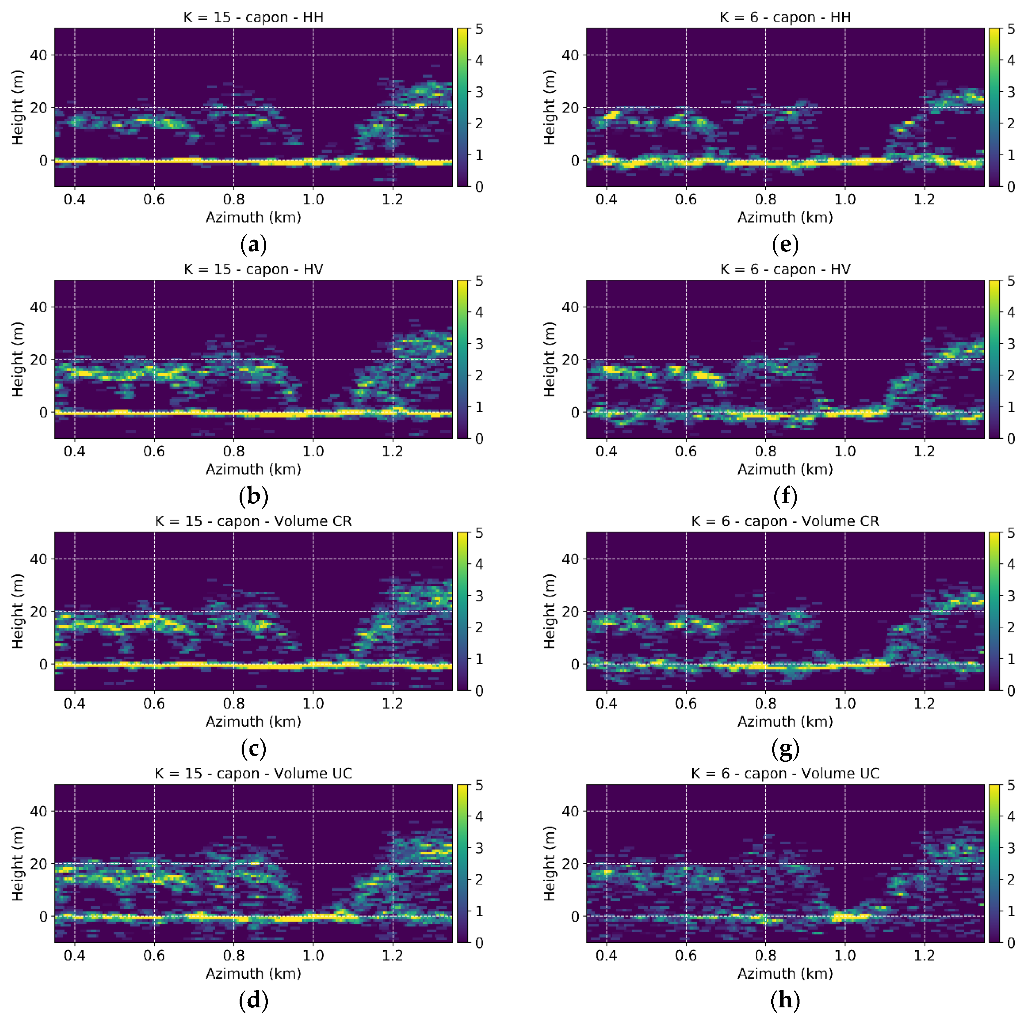In this Section, the robustness of the characterization of structure from Capon profiles is evaluated in a reduced scenario in which only $K=6$ images acquired along uniformly distributed tracks are available, but with a maximum displacement amounting to 1/3 of the full-stack case. As a consequence, the Rayleigh vertical resolution becomes 21 m at mid-range, i.e., three times worse than in the full-stack case. The largest volume occupies now around two height resolution units. The underlying L-band penetration and sensitivity to structure components does not change, but the ability to characterize them does. Figure 14 shows the Capon profiles obtained along the same azimuth line of Figure 3 with the reduced stack. The reduced vertical resolution is apparent, and not always peaks at different heights are separated from each other, additionally reducing the capability to distinguish the homogenous from the multilayered stands at the two sides of the transect.

The effect of the estimation of the ground height using the methodology discussed in Section 3 and implemented as discussed in Section 5 is evaluated first. Figure 6d shows the round height estimation error obtained using ${\tilde{\mathsf{\Gamma }}}_{G,CR}$, i.e., the maximized ground-to-volume ratio. A residual estimation error increasing from near to far range (e.g., in the direction of decreasing vertical resolution) is now apparent when compared to full-stack case. As the volume height compared to the Rayleigh resolution becomes lower, the overall bias increases to 3 m and the standard deviation to 6 m. The height error histograms in Figure 7b show that the poorer the vertical Rayleigh resolution, the stronger the ground contribution needs to be in order to achieve a certain ground height estimation performance. This makes the polarimetric optimization of the ground-to-volume ratio more important. Indeed, the optimization of the ground-to-volume ratio reduces the volume bias on the ground estimates reaching a minimum of around 2.3 m if the candidate solution closer to the unit circle is chosen. The increase of the standard deviation with respect to the better conditioned ${\tilde{\mathsf{\Gamma }}}_{G,CR}$ is negligible. Further, the error distribution in Figure 7b shows that a ground estimation error lower than 5 m can in this case be achieved with ${\mu }_{max}>-10$ dB provided that the volume-only Capon profiles have some contribution at the ground level. The bias associated to the loss of resolution increases the volume-only power measured by the Capon estimator at the ground with respect to the full-stack case. Recalling (14), this helps the detection of a ground peak with ${\mu }_{max}<-10$ dB, but with a significant loss of performance.

The estimation of the structure indices $HS$ and $VS$ now relies on the 3D distributions of peaks extracted from profiles with lower vertical resolution than in the full-stack case. The examples in Figure 9e–h show the changes across the polarization channels similar to the ones in the full-stack case. However, in the taller stands the reduction of resolution causes a larger concentration of peaks closer to the canopy top, since peaks at lower height are more difficult to be separated from the ground one. In turn, all the intermediate values of $HS$ become lower as shown in Figure 10c. On the other hand, volume peaks in shorter stands might be missed simply because they are not resolved from the ground. As a consequence, $HS$ can now reach higher values in these stands. Overall, the TomoSAR $HS$ is slightly positive biased and more dispersed with respect to the lidar $HS$, but the two are still in agreement (Figure 11c). As expected, a distribution of volume peaks in a narrower height interval leads to lower $VS$ values when compared to the full-stack case (Figure 12c), thus reducing the range of structure types that can be distinguished from each other. Similarly to $HS$, despite the slight negative bias and an increased standard deviation, the TomoSAR derived $VS$ still agrees with the lidar derived $VS$ (Figure 13c). Finally, consistently with the full-stack case, it appears that any polarization optimization does not really improve the ability to distinguish the different structure types from each other.

7. Effect of the TomoSAR Acquisition Implementation

Up to now the discussion has been based on TomoSAR acquisitions performed within few hours, guaranteeing the stationarity of the reflectivity. In these cases, even if the scatterers move due to wind, introducing temporal decorrelation, the underlying vertical reflectivity profile does not change. However, with longer observation times, the vertical reflectivity profile can change as a result of changing geometric and dielectric properties of the scattering distribution induced by, e.g., rainfalls, droughts, seasonality, disturbance, etc. Data sets of (realistic) space borne TomoSAR implementations will build up of images acquired within weeks or even months. In this case, reflectivity changes can occur from acquisition to acquisition, and the stationarity of the underlying reflectivity within the tomographic set is not anymore given [37]. Depending on the amount and nature of change, the resulting temporal decorrelation (in the sense of non-stationarity) of the underlying reflectivity can cause the defocusing of the estimated vertical profile independently of the used reconstruction algorithm with a consequential resolution and sidelobe level degradation [62].

The effect of such TomoSAR defocusing on the extraction of structure information from the estimated reflectivity profiles is addressed in this Section with respect to two different temporal decorrelation scenarios associated to two different TomoSAR acquisition implementations. In a conventional repeat-pass implementation each SLC image is acquired at a different time. In a bistatic implementation [20,26,63,64] each acquisition consists of (practically) simultaneously acquired pairs of images where each pair is acquired at a different time and with a different vertical wavenumber. Differently from the repeat-pass case, in the bistatic case temporal decorrelation (including the change of the underlying reflectivity) may occur between image pairs, but not within the same pair.

Figure 15 shows the interferometric coherences between the same reference tracks at different days together with the corresponding (residual) vertical wavenumber ${\kappa }_Z$ resulting from deviations from the nominal track. In addition, here the coherences have been calculated over 20 × 20 m range-azimuth multilook windows, corresponding to 500 (nominally) independent looks. The closer to zero ${\kappa }_Z$ is, the more the interferometric coherences express only temporal decorrelation. The highest coherences are obtained for the smallest time differences, i.e., between June 10 and June 16. Over baser areas the coherence is around 0.7 in average. In forested areas, the coherence decreases to 0.4 in those tall stands with large(r) ${\kappa }_Z$. Since volumetric and temporal effects cannot be separated, this value may actually contain a significant volume decorrelation contribution. This conclusion is supported by the work in [65]. The lowest coherences are obtained for the larger time difference, i.e., between May 20 and July 28. In this case, bare areas exhibit low coherence (around 0.35), while in the forest stands the coherence does not drop below 0.35. However, a larger time interval does not necessarily imply a lower coherence. For instance, the coherence for the pair (J May 20, July 28,) reaches similar decorrelation levels to the ones for the pair (May 20, Jun 10) despite the 1 month longer separation. However, the decorrelation in the (May 20, June 10) pair might include also residual volumetric effects as indicated by the higher ${\kappa }_Z$. The largest mean coherence in forested areas has been found for the pair (June 20, July 28) about 0.45.

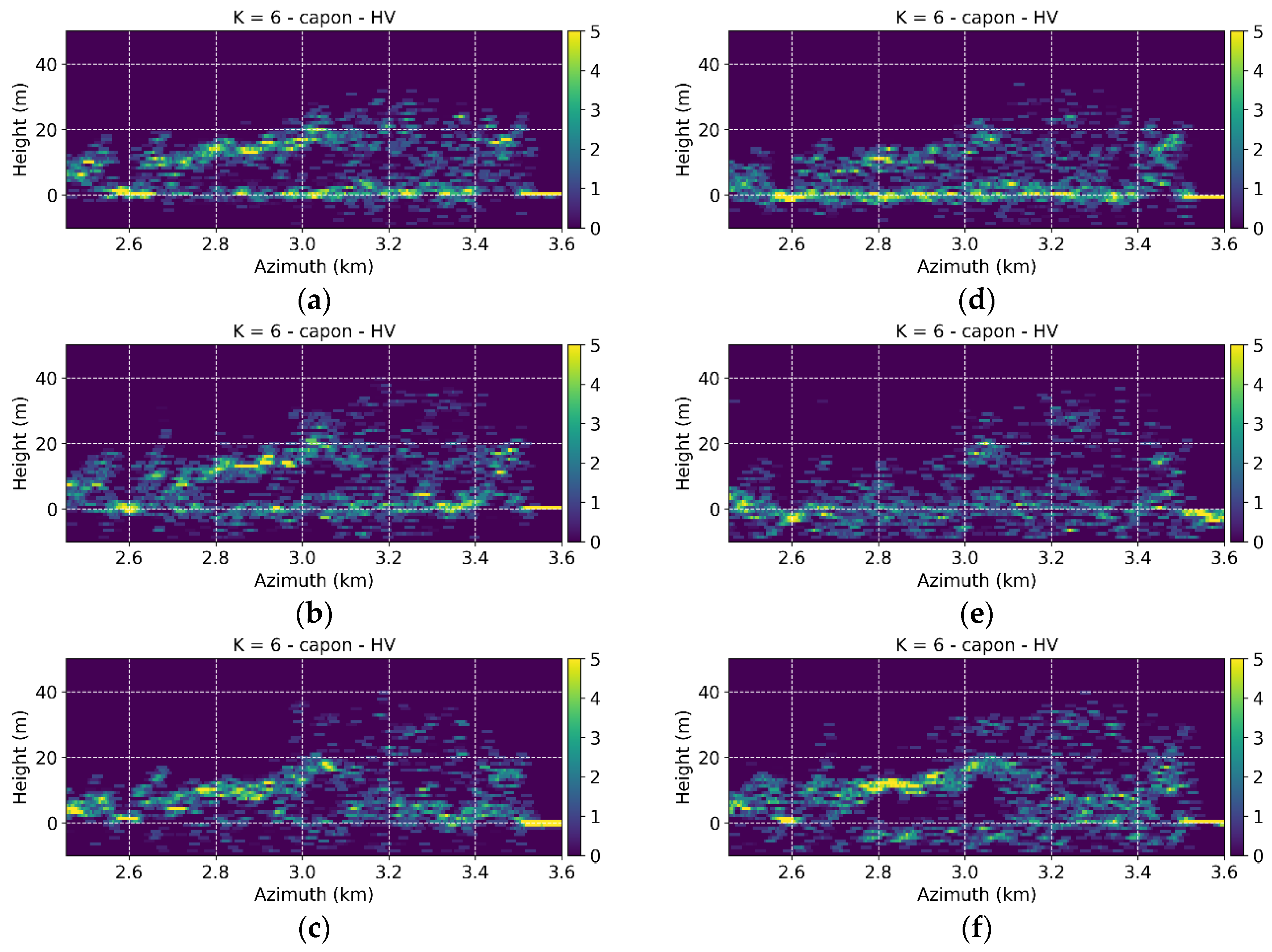
Capon profiles have been generated using the coherences matrices after interpolation in multilook cells of 5 × 5 m (corresponding to 30 nominal independent looks). Following the same procedure as in Section 3 and Section 5, the structure indices are estimated. Figure 16a–d shows the number of peaks in the HV channel in every 5 × 1 m azimuth-height bin along an azimuth transect for the four acquisition dates. The transect crosses mature (until an azimuth distance of 3 km) and “Plenterwald” stands. On May 20, a higher concentration of peaks appears at ground level heights, while vegetation peaks tend to be sparsely distributed. It is expected that the two forest types are more distinct in terms of vertical structure rather than of horizontal structure. As spring progresses towards summer (from May 20 to July 28), the profile peaks concentrate more and more towards the canopy top, especially in the mature stands. These stands become now more distinguishable also in terms of horizontal heterogeneity. This agrees with what observed and reported in [37] and could be an indication for the seasonal redistribution of water in the tree tissues: while in spring the water is more present in the tree trunks, in summer transpiration phenomena concentrate water towards the canopy top. There is a stronger reflectivity change between May 20 and June 10 than between the June and July, that agrees with the temporal decorrelation maps of Figure 17.

A repeat-pass TomoSAR data set is synthesized by combining after interpolation SLC’s from different days with wavenumbers decreasing with time (see Table 1). The transect obtained is shown in Figure 15e. Supported also by the analysis in [26], the defocusing caused by the presence of temporal decorrelation over such a large time span degrades the estimated volume scattering components making a distinction between them difficult if not impossible. As a result, the structural characteristics of the two stands cannot be retrieved anymore. The bistatic implementation has been emulated by considering a set of coherences with the same decrease of wavenumber in time similar as in the repeat-pass case. Following the procedure detailed in [20,26,63,64], a coherence matrix can be built up with a coherence set with uniformly distributed wavenumbers following a Toeplitz form. The Capon estimator can be applied to the reconstructed coherence matrix, and the structure indices calculated. The corresponding transect is shown in Figure 16f indicating that complex coherences measured in a bistatic implementation can make L-band structure characterization robust to the underlying temporal reflectivity changes. The change of the vertical distribution of peaks along azimuth now reflects the structural difference between the two stands.

The comparison between the three TomoSAR configurations (single-pass, repeat-pass and bistatic) is extended to the whole site in Figure 17 and Figure 18 for the horizontal and vertical structure indices. The data set of July 28 has been reported as a reference “single-pass” one with no reflectivity changes between acquisitions. The spatial trends of both HS and $VS$ correlate with the growth stage patterns in Figure 19a [23,53]. To help the interpretation, in Figure 19b the mean values of $VS$ and $HS$ for each stage are plotted one as a function of the other for the four acquisition dates. Mature and growing stands are comparable in terms of $VS$, but the decreasing density of the growing stands is reflected in a higher $HS$. $HS$ increases further in the young stands due to the lower density where $VS$ increases as well. These three stages are then well distinguishable from the transition and “Plenterwald” stands thanks to the large difference in $VS$. For the two latter stages, $HS$ remains on intermediate values—larger than in mature stands, but lower than young ones. However, they are structurally equivalent. These characteristics are unaltered across the acquisition dates, but the single mean values of $HS$ and $VS$ can present some variability with acquisition time along the seasonal change. Recalling what already commented for the transects in Figure 18, the two furthest points along the $VS$ axis on July 28 represented by the mature and the “Plenterwald” stands become closer on May 20 and June 10 than on July 28. However, on July 28 mature and growing stands they become the closest in terms of $HS$, while they are the most separated ones in terms of $HS$ in the May 20 and in the June 20 acquisitions. The spatial structural gradients (Figure 17b and Figure 18b) and their relationships across the different growth stages (Figure 19c) are lost in the repeat-pass case as the defocusing drives many profile peaks below the amplitude threshold making almost all stands to appear heterogeneous horizontally and homogeneous vertically. In contrast, the robustness of the bistatic implementation to the underlying L-band reflectivity changes allows to retrieve meaningful structural relationships (Figure 17c, Figure 18c and Figure 19c) very well within the variability of the four data sets representing the single-pass case.

8. Discussion and Conclusions

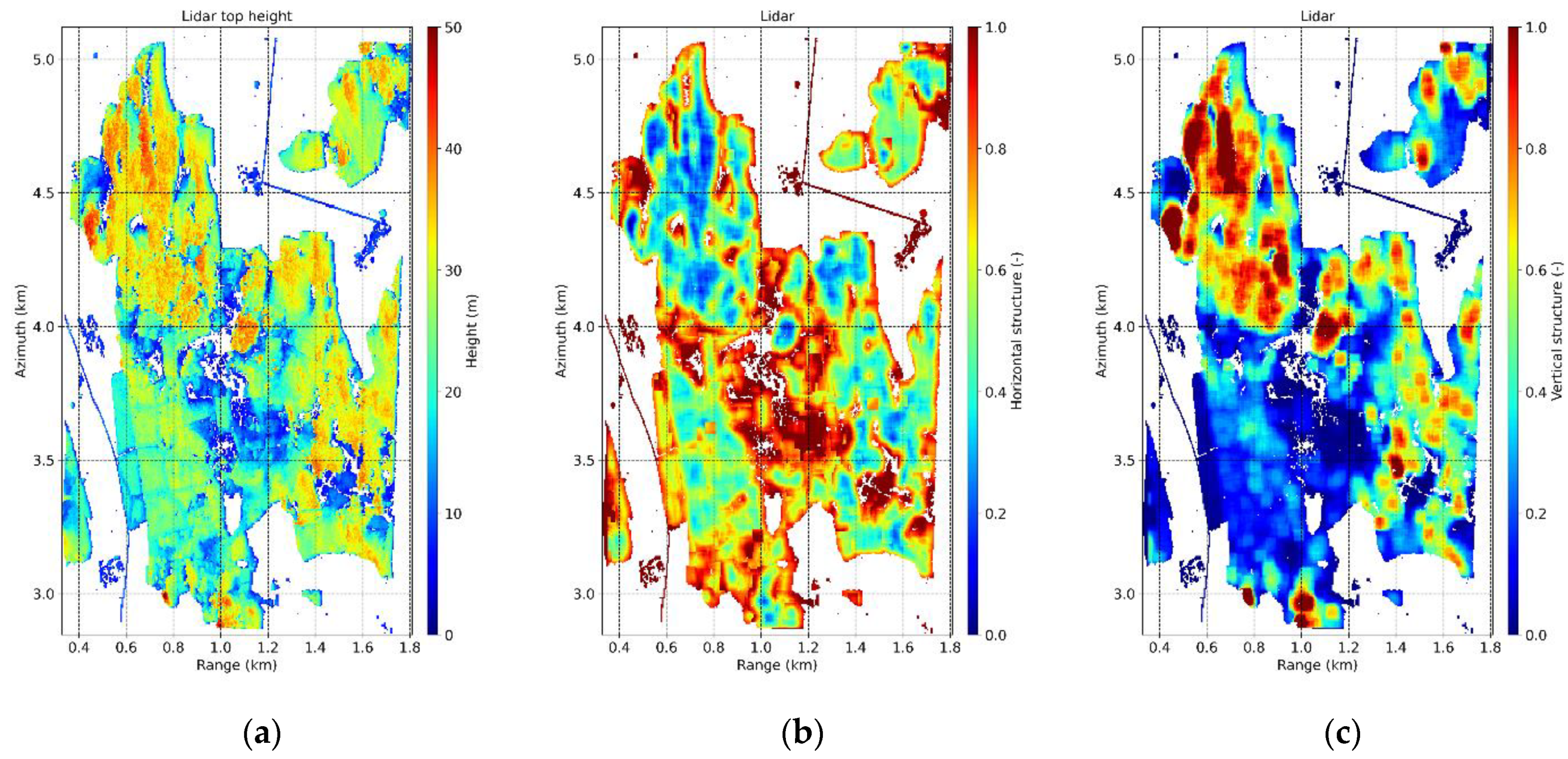
In this paper, the potential of tomographically reconstructed L-band reflectivity for the (qualitative and quantitative) characterization of 3D forest structure has been reviewed and discussed not only with respect to the information content of the reconstructed reflectivity, but also regarding the tomographic acquisition configuration and implementation. The analysis has been carried out by processing airborne L-band TomoSAR data acquired over the temperate forest of Traunstein (south of Germany). The reconstruction was performed by applying the conventional Capon spectral estimator to the different data sets. The experiments in this paper confirm that L-band is able to penetrate until the ground even through the dense and tall forest stands, while remains sensitive enough to the distribution of the smaller canopy elements that determine the 3D structure. The horizontal and vertical forest structure is described by a pair of complementary indices derived from the distribution of the peaks of the reconstructed reflectivity within a given structure window (on the order of a quarter of hectare). The ability to fully characterize both dimensions has been confirmed by comparing the obtained index values with the ones derived by lidar and is supported by other experiments reported in the literature where also the correspondence to equivalent structure indices derived from ground inventory measurements has been established [24]. L-band structure measurements by means of TomoSAR are of course not limited to temperate forests and have already been demonstrated in tropical as well as in boreal forest sites [22]. A high(er) vertical resolution becomes critical in order to identify both the weak(er) ground and those relevant, vegetation scattering contributions in the lowest stand compartments [14,22]. Together with a large(r) number of images, it also facilitates the reconstruction of more complex reflectivity profiles [22,66]. The effect of non-optimal TomoSAR configurations in terms of lower vertical resolution and higher level of sidelobes on the reconstructed reflectivity can be counteracted by employing super-resolution estimators like, e.g., compressive sensing. The characterization of structure also benefits from high(er) range-azimuth resolutions. On the one hand, the vertical reflectivity reconstruction is more accurate due to the larger number of independent looks available for a certain multilook cell size. On the other hand, the calculation of structure indices is more robust as each structure window includes a larger number of (independent) reflectivity samples (e.g., profiles) within an area that is still meaningful for heterogeneous stands.

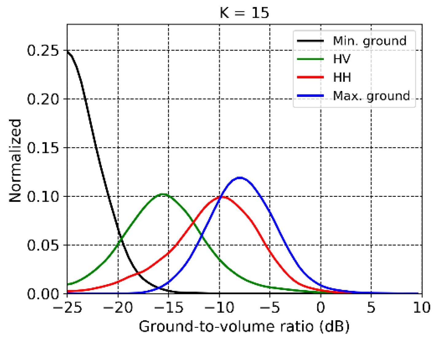
Within the RVoG hypothesis, the change of the polarimetric channel implies a change of the ground-to-volume ratio. The “visibility” of the polarized ground at L-band makes this change significant. For a fixed vertical point-spread function defined by the TomoSAR configuration, the ability to increase the ground-to-volume ratio by changing the polarization channel becomes relevant because it (1) increases the detectability of the ground peak in the TomoSAR profiles regardless of the contribution of close to ground vegetation components to reflectivity and (2) improves the performance of estimating its position by reducing the vegetation-induced bias. In Froschham, the ground-to-volume ratio increases by 5 dB in average from HV to HH. For an ideal regular track configuration with vertical resolution better than 10 m, this increase allows a complete compensation of the vegetation-induced ground height bias and of the reduction of the standard deviation by around 40% (to lower than 3 m). Polarimetric interferometric [48,59] optimization techniques can increase the ground-to-volume ratio by 3 dB in average. This is in many cases enough to ensure a robust and accurate ground detection. For example, the estimation error reduces from 4 m in HH to 2 m. Polarization diversity becomes even more critical for those TomoSAR configurations with a rather low vertical resolution. The experiments in Froschham showed that for a reduced-stack configuration allowing a vertical resolution of about 20 m, the vegetation bias is reduced by almost 50% when changing from HV to HH. The polarimetric maximization of the ground-to-volume ratio reduces the bias by additional 30%, while the (very) limited resolution prevents any further improvement. The standard deviation reaches 6 m in this case.

Still under the RVoG hypothesis, even for an infinite TomoSAR vertical resolution, the choice of the polarization channel would have no effect on the estimation of the horizontal and vertical structure indices as the estimated vegetation reflectivity components would not change. This is indeed confirmed at a large extent by simply comparing the experimental results obtained in HH and HV using the full-stack configuration in the Traunstein forest. The small residual difference is caused by the performance of the TomoSAR imaging in focusing weak(er) scatterers (here volume components weaker in HH than in HV), but also by a sub-optimum amplitude threshold used for the selection of the meaningful peaks. As a consequence, the detected “meaningful” peaks in HH tend to be concentrated closer to the ground than in HV, resulting into a slight (10%) bias in the horizontal structure and a slightly higher dispersion in the vertical structure. A further polarimetric interferometric optimization to minimize the ground scattering contribution does not lead to any significant improvement compared to HV, as it is reasonable to expect. Two factors affect the structure indices values at a larger extent. First, a reduction of the Rayleigh vertical resolution reduces the range of values of the structure indices and/or their distribution, especially in the vertical direction. Employing a spatially larger structure window may increase robustness, as long as it is still appropriate to represent structure variations. If this is the case, then the Capon (or in some cases) even the Fourier-based reconstructions might be used. However, if a smaller structure window is needed, better performing estimators (like, e.g., compressive sensing) need to be employed for reconstructing the reflectivity. Second, it has been seen that the L-band sensitivity to seasonal changes, as for example caused by the re-distribution of the water content within the tree tissues occurring within in a time span of 2 months between spring and summer may change the peak distribution and lead to (slightly) different structure index values. However, this change does not significantly impact the capability to discriminate among different forest stands. This robustness is definitely enhanced by using reflectivity peak positions rather than reflectivity values itself [24,37].

The robustness to the temporal decorrelation effects induced by possible changes of the reflectivity in time also drives the choice of the implementation of the TomoSAR acquisitions in space borne scenarios. The experimental results have shown that the long-term seasonal variations at L-band violate the stationarity assumption, and a simple decay with time may not be sufficient to describe them. In contrast to a conventional repeat-pass implementation, a bistatic-like TomoSAR implementation in which a temporal decorrelation-free complex coherence measurement is obtained at each revisit appears to be robust against the seasonal change of vertical reflectivity in a 2-month time span, and able to restore the capability to discriminate the different structure types. It is worth noting that in the case of space borne implementations the ability to perform all the required acquisitions in the minimum possible time becomes relevant for minimizing the effects of seasonal reflectivity changes. For instance, a revisit time in the order of 1 week or less could allow the estimation of structure parameters at L-band even in a repeat-pass mode [65,66].

It is anticipated that the experiments described in this paper trigger a more general characterization of the potential of L-band SAR tomography for forest structure mapping. The presented structure framework is just a first step towards the interpretation of TomoSAR measurements in terms of physical 3D structure. The development of such a framework is essential not only in light of a number of planned or proposed L-band missions aiming at forest monitoring (e.g., NASA’s NISAR [67], ESA’s ROSE-L [68] and DLR’s Tandem-L [69]), but also to better shape acquisition requirements and finally initiate novel information products able even to accommodate synergies and complementarities with measurements at different SAR and lidar wavelengths.

References

1. Parker, G.G. Structure and microclimate of forest canopies. In Forest Canopies—A Review of Research on a Biological Frontier; Lowman, M., Nadkarni, N., Eds.; Elsevier Academic Press: Amsterdam, The Netherlands, 2004; pp. 73–106. [Google Scholar]
2. Lefsky, M.A.; Harding, D.J.; Cohen, W.B.; Parker, G.G.; Shugart, H.H. Surface lidar remote sensing of basal area and biomass in deciduous forests of eastern Maryland, USA. Remote Sens. Environ. 1999, 67, 83–98. [Google Scholar] [CrossRef]
3. Spies, T.A. Forest structure: A key to the ecosystem. Northwest Sci. 1998, 72, 34–36. [Google Scholar]
4. Harding, D.J.; Lefsky, M.A.; Parker, G.G.; Blair, J.B. Laser altimeter canopy height profiles—Methods and validation for closed-canopy, broadleaf forest. Remote Sens. Environ. 2001, 76, 283–297. [Google Scholar] [CrossRef]
5. Snyder, M. What is forest stand structure and how is it measured? North. Woodl. 2010, 64, 15. [Google Scholar]
6. Hall, F.G.; Bergen, K.; Blair, J.B.; Dubayah, R.; Houghton, R.; Hurtt, G.; Kellndorfer, J.; Lefsky, M.; Ranson, J.; Saatchi, S.; et al. Characterizing 3D vegetation structure from space: Mission requirements. Remote Sens. Environ. 2011, 115, 2753–2775. [Google Scholar] [CrossRef] [Green Version]
7. Brokaw, N.; Lent, R. Vertical Structure. In Maintaining Biodiversity in Forest Ecosystems; Hunter, M.L., Jr., Ed.; Cambridge University Press: Cambridge, UK, 1999; pp. 373–399. [Google Scholar]
8. McElhinny, C.; Gibbons, P.; Brack, C.; Bauhus, J. Forest and woodland stand structural complexity: Its definition and measurement. For. Ecol. Manag. 2005, 218, 1–24. [Google Scholar] [CrossRef]
9. Bohn, F.J.; Huth, A. The importance of forest structure to biodiversity-productivity relationships. R. Soc. Open Sci. 2017, 4, 160521. [Google Scholar] [CrossRef] [PubMed] [Green Version]
10. Bergen, K.M.; Goetz, S.J.; Dubayah, R.O.; Henebry, G.M.; Hunsaker, C.T.; Imhoff, M.L.; Nelson, R.F.; Parker, G.G.; Radeloff, V.C. Remote sensing of vegetation 3-D structure for biodiversity and habitat: Review and implications for lidar and radar spaceborne missions. J. Geophys. Res. 2009, 114, G00E06. [Google Scholar] [CrossRef] [Green Version]
11. Goetz, S.; Steinberg, D.; Dubayah, R.O.; Blair, B. Laser remote sensing of canopy habitat heterogeneity as a predictor of bird species richness in an eastern temperate forest. Remote Sens. Environ. 2007, 108, 254–263. [Google Scholar] [CrossRef]
12. Turner, W.; Spector, S.; Gardiner, N.; Fladeland, M.; Sterling, E.; Steininger, M. Remote sensing for biodiversity science and conser-vation. Trend Ecol. Evol. 2003, 18, 306–314. [Google Scholar] [CrossRef]
13. Frolking, S.; Palace, M.W.; Clark, D.B.; Chambers, J.Q.; Shugart, H.H.; Hurtt, G.C. Forest disturbance and recovery: A general review in the context of spaceborne remote sensing of impacts on aboveground biomass and canopy structure. J. Geophys. Res. 2009, 114, G00E02. [Google Scholar] [CrossRef]
14. Pardini, M.; Armston, J.; Qi, W.; Lee, S.K.; Tello-Alonso, M.; Cazcarra-Bes, V.; Choi, C.; Papathanassiou, K.; Dubayah, R.; Fatoyinbo, L.E. Early Lessons on Combining Lidar and Multi-baseline SAR Measurements for Forest Structure Characterization. Surv. Geophys. 2019, 40, 803–837. [Google Scholar] [CrossRef]
15. Moreira, A.; Prats-Iraola, P.; Younis, M.; Krieger, G.; Hajnsek, I.; Papathanassiou, K. A tutorial on synthetic aperture radar. IEEE Geosci. Remote Sens. Mag. 2013, 1, 6–43. [Google Scholar] [CrossRef] [Green Version]
16. Reigber, A.; Moreira, A. First demonstration of airborne SAR tomography using multibaseline L-band data. IEEE Trans. Geosci. Remote Sens. 2000, 38, 2142–2152. [Google Scholar] [CrossRef]
17. Lombardini, F.; Pardini, M. Experiments of tomography-based SAR techniques with P-band polarimetric data. In Proceedings of the 2009 ESA International workshop on polarimetry and Polarimetric Interferometry (POLinSAR), Frascati, Italy, 26–30 January 2009. [Google Scholar]
18. Frey, O.; Meier, E. Analyzing tomographic SAR data of a forest with respect to frequency, polarization, and focusing technique. IEEE Trans. Geosci. Remote Sens. 2011, 49, 3648–3659. [Google Scholar] [CrossRef] [Green Version]
19. Tebaldini, S.; Rocca, F. Multibaseline Polarimetric SAR Tomography of a Boreal Forest at Pand L-bands. IEEE Trans. Geosci. Remote Sens. 2012, 50, 232–246. [Google Scholar] [CrossRef]
20. Nannini, M.; Martone, M.; Rizzoli, P.; Prats-Iraola, P.; Rodriguez-Cassola, M.; Reigber, A.; Moreira, A. Coherence-based SAR tomography for spaceborne applications. Remote Sens. Environ. 2019, 225, 107–114. [Google Scholar] [CrossRef] [Green Version]
21. Lavalle, M.; Hawkins, B.; Hensley, S. Tomographic imaging with UAVSAR: Current status and new results from the 2016 AfriSAR campaign. In Proceedings of the 2017 IEEE International Geoscience and Remote Sensing Symposium (IGARSS), Fort Worth, TX, USA, 23–28 July 2017. [Google Scholar]
22. Pardini, M.; Tello, M.; Cazcarra-Bes, V.; Papathanassiou, K.; Hajnsek, I. L- and P-band 3-D SAR reflectivity profiles versus lidar waveforms: The AfriSAR case. IEEE J. Sel. Top. Appl. Earth Obs. Remote Sens. 2018, 11, 3386–3401. [Google Scholar] [CrossRef]
23. Cazcarra Bes, V.; Tello, M.; Fischer, R.; Heym, M.; Papathanassiou, K. Monitoring forest structure dynamics by means of L-band SAR tomography. Remote Sens. 2017, 9, 1229. [Google Scholar] [CrossRef] [Green Version]
24. Tello, M.; Cazcarra-Bes, V.; Pardini, M.; Papathanassiou, K. Forest structure characterization from SAR tomography at L-band. IEEE J. Sel. Top. Appl. Earth Obs. Remote Sens. 2018, 11, 3402–3414. [Google Scholar] [CrossRef] [Green Version]
25. Kugler, F.; Lee, S.K.; Hajnsek, I.; Papathanassiou, K. Forest height estimation by means of Pol-InSAR data inversion: The role of the vertical wavenumber. IEEE Trans. Geosci. Remote Sens. 2015, 53, 5294–5311. [Google Scholar] [CrossRef]
26. Cazcarra-Bes, V.; Pardini, M.; Tello, M.; Papathanassiou, K. Comparison of tomographic SAR reflectivity reconstruction algorithms for forest applications at L-band. IEEE Trans. Geosci. Remote Sens. 2020, 58, 147–164. [Google Scholar] [CrossRef]
27. Capon, J. High-resolution frequency-wavenumber spectrum analysis. Proc. IEEE 1969, 57, 1408–1418. [Google Scholar] [CrossRef] [Green Version]
28. Lombardini, F.; Reigber, A. Adaptive spectral estimation for multibaseline SAR tomography with airborne L-band data. In Proceedings of the 2003 IEEE International Geoscience and Remote Sensing Symposium, Toulouse, France, 21 July 2003. [Google Scholar]
29. Stoica, P.; Moses, R. Spectral Analysis of Signals; Prentice Hall: Englewook Cliffs, NJ, USA, 2005. [Google Scholar]
30. Marzetta, L. A new interpretation for Capon’s maximum likelihood method of frequency-wavenumber spectral estimation. IEEE Trans. Acoust. Speech Signal Process. 1983, 31, 445–449. [Google Scholar] [CrossRef]
31. Hassanien, A.; Shahbazpanahi, A.; Gershman, A.B. A generalized Capon estimator for localization of multiple spread sources. IEEE Trans. Signal Process. 2006, 52, 280–283. [Google Scholar] [CrossRef]
32. Lombardini, F.; Cai, F. Generalized-capon method for Diff-Tomo SAR analyses of decorrelating scatterers. Remote Sens. 2019, 11, 412. [Google Scholar] [CrossRef] [Green Version]
33. Cloude, S. Polarization coherence tomography. Radio Sci. 2006, 41, RS4017. [Google Scholar] [CrossRef]
34. Aguilera, E.; Nannini, M.; Reigber, A. A data-adaptative compressed sensing approach to polarimetric SAR tomography of forested areas. IEEE Trans. Geosci. Remote Sens. Lett. 2013, 10, 543–547. [Google Scholar] [CrossRef]
35. Aghababaee, H.; Ferraioli, G.; Ferro-Famil, L.; Schirinzi, G.; Huang, Y. Sparsity based full rank polarimetric reconstruction of coherence matrix T. Remote Sens. 2019, 11, 1288. [Google Scholar] [CrossRef] [Green Version]
36. Huang, Y.; Levy-Vehel, J.; Ferro-Famil, L.; Reigber, A. Three-dimensional imaging of objects concealed below a forest canopy using SAR tomography at L-band and wavelet-based sparse estimation. IEEE Geosci. Remote Sens. Lett. 2017, 14, 1454–1458. [Google Scholar] [CrossRef]
37. Pardini, M.; Papathanassiou, K.; Lombardini, F. Impact of dielectric changes on L-band 3-D SAR reflectivity profiles of forest volumes. IEEE Trans. Geosci. Remote Sens. 2018, 56, 7324–7337. [Google Scholar] [CrossRef]
38. D’Hondt, O.; Hänsch, R.; Wagener, N.; Hellwich, O. Exploiting SAR tomography for supervised land-cover classification. Remote Sens. 2018, 10, 1742. [Google Scholar] [CrossRef] [Green Version]
39. Ho Tong Minh, D.; Le Toan, T.; Rocca, F.; Tebaldini, S.; Mariotti d’Alessandro, M.; Villard, L. Relating P-band synthetic aperture radar tomography to tropical forest biomass. IEEE Trans. Geosci. Remote Sens. 2014, 52, 967–979. [Google Scholar] [CrossRef]
40. Toraño Caicoya, A.; Pardini, M.; Hajnsek, I.; Papathanassiou, K. Forest above-ground biomass estimation from vertical reflectivity profiles at L-band. IEEE Geosci. Remote Sens. Lett. 2015, 12, 2379–2383. [Google Scholar] [CrossRef]
41. Blomberg, E.; Ferro-Famil, L.; Soja, M.J.; Ulander, L.M.H.; Tebaldini, S. Forest biomass retrieval from L-band SAR using tomographic ground backscatter removal. IEEE Geosci. Remote Sens. Lett. 2018, 15, 1030–1034. [Google Scholar] [CrossRef]
42. Mariotti D’Alessandro, M.; Tebaldini, S. Digital terrain model retrieval in tropical forests through P-band SAR tomography. IEEE Trans. Geosci. Remote Sens. 2019, 57, 6774–6781. [Google Scholar] [CrossRef]
43. Yang, X.; Tebaldini, S.; Mariotti d’Alessandro, M.; Liao, M. Tropical forest height retrieval based on P-band multibaseline SAR data. IEEE Geosci. Remote Sens. Lett. 2020, 17, 451–455. [Google Scholar] [CrossRef]
44. Brolly, M.; Woodhouse, I.H. Vertical backscatter profile of forests predicted by a macroecological plant model. Int. J. Remote Sens. 2013, 34, 1026–1040. [Google Scholar] [CrossRef] [Green Version]
45. Thirion, L.; Colin, E.; Dahon, C. Capabilities of a forest coherent scattering model applied to radiometry, interferometry, and polarimetry at P- and L-Band. IEEE Trans. Geosci. Remote Sens. 2006, 44, 849–862. [Google Scholar] [CrossRef]
46. Lin, Y.; Sarabandi, K. A Monte Carlo coherent scattering model for forest canopies using fractal-generated trees. IEEE Trans. Geosci. Remote Sens. 1999, 37, 440–451. [Google Scholar]
47. Treuhaft, R.N.; Siqueira, P.R. Vertical structure of vegetated land surfaces from interferometric and polarimetric radar. Radio Sci. 2000, 35, 141–177. [Google Scholar] [CrossRef] [Green Version]
48. Papathanassiou, K.; Cloude, S. Single-baseline polarimetric SAR interferometry. IEEE Trans. Geosci. Remote Sens. 2001, 39, 2352–2363. [Google Scholar] [CrossRef] [Green Version]
49. Jakobsson, A.; Gini, F.; Lombardini, F. Robust estimation of radar reflectivities in multibaseline InSAR. IEEE Trans. Aerosp. Electr. Syst. 2005, 41, 751–758. [Google Scholar] [CrossRef]
50. Pardini, M.; Lombardini, F.; Gini, F. The hybrid Cramér–Rao bound on broadside DOA estimation of extended sources in presence of array errors. IEEE Trans. Signal Process. 2008, 56, 1726–1730. [Google Scholar] [CrossRef]
51. Available online: https://forestgeo.si.edu/sites/europe/traunstein (accessed on 14 March 2021).
52. Reigber, A.; Scheiber, R.; Jäger, M.; Prats-Iraola, P.; Hajnsek, I.; Jagdhuber, T.; Papathanassiou, K.; Nannini, M.; Aguilera, E.; Baumgartner, S.; et al. Very-high-resolution airborne synthetic aperture radar imaging: Signal processing and applications. Proc. IEEE 2013, 101, 759–783. [Google Scholar] [CrossRef] [Green Version]
53. Wallner, A.; Elatawneh, A.; Schneider, T.; Knoke, T. Estimation of forest structural information using RapidEye satellite data. For. Int. J. For. Res. 2015, 88, 96–107. [Google Scholar] [CrossRef] [Green Version]
54. Bordoni, F.; Jakobsson, A.; Lombardini, F.; Gini, F. Multibaseline cross-track SAR interferometry using interpolated arrays. IEEE Trans. Aerosp. Electr. Syst. 2005, 41, 1473–1482. [Google Scholar] [CrossRef]
55. Lombardini, F.; Pardini, M. 3-D SAR tomography: The multibaseline sector interpolation approach. IEEE Geosci. Remote Sens. Lett. 2008, 5, 630–634. [Google Scholar] [CrossRef]
56. Tebaldini, S. Algebraic synthesis of forest scenarios from multibaseline PolInSAR data. IEEE Trans. Geosci. Remote Sens. 2009, 47, 4132–4142. [Google Scholar] [CrossRef]
57. Pardini, M.; Papathanassiou, K. On the estimation of ground and volume polarimetric covariances in forest scenarios with SAR tomography. IEEE Geosci. Remote Sens. Lett. 2017, 14, 1860–1864. [Google Scholar] [CrossRef] [Green Version]
58. Tebaldini, S.; Rocca, F. Coherence linearity and SKP-structured matrices in multi-baseline PolInSAR. In Proceedings of the 2011 IEEE International Geoscience and Remote Sensing Symposium, Vancouver, BC, Canada, 24–29 July 2011. [Google Scholar]
59. Cloude, S.; Papathanassiou, K. Three-stage inversion process for polarimetric SAR interferometry. IEE Proc. Radar Sonar Navig. 2003, 150, 125–134. [Google Scholar] [CrossRef] [Green Version]
60. Ferro-Famil, L.; Huang, Y.; Neumann, M. Robust estimation of Multi-Baseline POL-inSAR parameters for the analysis of natural environments. In Proceedings of the 8th European Conference on Synthetic Aperture Radar, Aachen, Germany, 7–10 June 2010. [Google Scholar]
61. Cazcarra-Bes, V.; Pardini, M.; Papathanassiou, K. Definition of tomographic SAR configurations for forest structure applications at L-band. IEEE Geosci. Remote Sens. Lett. 2020. [Google Scholar] [CrossRef]
62. Lombardini, F.; Cai, F. Temporal decorrelation-robust SAR tomography. IEEE Trans. Geosci. Remote Sens. 2014, 52, 5412–5421. [Google Scholar] [CrossRef]
63. Pardini, M.; Toraño-Caicoya, A.; Kugler, F.; Papathanassiou, K. Estimating and understanding vertical structure of forests from multibaseline TanDEM-X Pol-InSAR data. In Proceedings of the 2013 IEEE International Geoscience and Remote Sensing Symposium—IGARSS, Melbourne, VIC, Australia, 21–26 July 2013. [Google Scholar]
64. Tebaldini, S.; Ferro-Famil, L. SAR tomography from bistatic single-pass interferometers. In Proceedings of the 2017 IEEE International Geoscience and Remote Sensing Symposium (IGARSS), Fort Worth, TX, USA, 23–28 July 2017. [Google Scholar]
65. Lee, S.K.; Kugler, F.; Papathanassiou, K.; Hajnsek, I. Quantification of temporal decorrelation effects at L-band for polarimetric SAR interferometry applications. IEEE J. Sel. Top. Appl. Earth Obs. Remote Sens. 2013, 6, 1351–1367. [Google Scholar] [CrossRef]
66. Pardini, M.; Papathanassiou, K. Spaceborne SAR tomography over forests: Performance and trade-offs for repeated single pass PolInSAR acquisitions. In Proceedings of the 2015 IEEE International Geoscience and Remote Sensing Symposium (IGARSS), Milan, Italy, 26–31 July 2015. [Google Scholar]
67. Rosen, P.; Kim, Y.; Kumar, R.; Misra, T.; Bhan, R.; Raju Sagi, V. Global persistent SAR sampling with the NASA-ISRO SAR (NISAR) mission. In Proceedings of the 2017 IEEE Radar Conference (RadarConf), Seattle, WA, USA, 8–12 May 2017. [Google Scholar]
68. Davidson, M.; Gebert, N.; Giulicchi, L. ROSE-L—The L-band SAR Mission for Copernicus. In Proceedings of the European Conference on Synthetic Aperture Radar (EUSAR), online event, 30 March–1 April 2021. [Google Scholar]
69. Moreira, A.; Krieger, G.; Hajnsek, I.; Papathanassiou, K.; Younis, M.; Lopez Dekker, P.; Huber, S.; Villano, M.; Pardini, M.; Eineder, M.; et al. Tandem-L: A highly innovative bistatic SAR mission for global observation of dynamic processes on the Earth’s surface. IEEE Geosci. Remote Sens. Mag. 2015, 3, 8–23. [Google Scholar] [CrossRef]
Figure 1. (a) Locations depicted (yellow polygons) on a Google Earth image, and Pauli images corresponding to the sites covered by the processed data sets (b) Froschham forest (northern yellow polygon) and (c) Traunstein “Bürgerwald” forest (southern yellow polygon). The yellow lines in (b,c) indicate the locations of transects considered for the examples in Section 5, Section 6 and Section 7.
Remotesensing 13 02255 g001
Figure 2. Froschham test site: lidar (a) top height (maximum height in 5 × 5 m), and structure indices (50 × 50 m) (b) H S and (c) V S .
Remotesensing 13 02255 g002
Figure 3. Froschham test site. L-band Capon profiles of coherence matrices (multilook 20 × 20 m) in the full K = 15 case in the (a) HH and (b) HV polarizations and using (c) Γ ˜ G , C R , (d) Γ ˜ V , C R , (e) Γ ˜ G , U C and (f) Γ ˜ V , U C . The height axis is referred to the ground topography. The location of the transect is shown in Figure 1b.
Remotesensing 13 02255 g003
Figure 4. Froschham test site. L-band ground-to-volume ratios (multilook 20 × 20 m) with K = 15 in the (a) HV, (b) HH and (c) maximum ground polarization channels.
Remotesensing 13 02255 g004
Figure 5. Froschham test site. Histograms of the estimated L-band ground-to-volume ratios in the different polarimetric channels.
Remotesensing 13 02255 g005
Figure 6. Froshham test site. Ground estimation error maps obtained using the L-band Capon profiles (multilook 20 × 20 m) with (a) K = 15 in HV, (b) K = 15 in HH, (c) K = 15 for Γ ˜ G , C R and (d) K = 6 for Γ ˜ G , C R .
Remotesensing 13 02255 g006
Figure 7. Froschham test site. Histograms of the L-band ground estimation errors in the forest areas in HH, HV, VV and using Γ ˜ G , C R and Γ ˜ G , U C with (a) K = 15 , and (b) K = 6 .
Remotesensing 13 02255 g007
Figure 8. Froschham test site. Distribution of the L-band ground estimation errors obtained using Γ ˜ G , C R in the plane inviduated by the corresponding ground-to-volume ratio and the volume-only Capon amplitude at the ground level, with (a) K = 15 and (b) K = 6 . Only the profiles with a ground peak have been considered.
Remotesensing 13 02255 g008
Figure 9. Froschham test site. Distributions of the selected peaks of the Capon profiles (multilook 10 × 10 m) using a 50 × 50 m structure window in the full K = 15 case in the reduced K = 6 case. (a,e): HH; (b,f): HV polarizations; (c,g): using Γ ˜ V , C R ; (d,h): using Γ ˜ V , U C . The height axis is referred to the ground topography. The location of the transect is shown in Figure 1b.
Remotesensing 13 02255 g009
Figure 10. Froshham test site. L-band TomoSAR horizontal structure H S (50 × 50 m) from Capon profiles with (a) K = 15 in HH, (b) K = 15 in HV and (c) K = 6 in HV.
Remotesensing 13 02255 g010
Figure 11. Froschham test site. 2-D histogram comparing the L-band TomoSAR and the lidar H S (50 × 50 m) with (a) K = 15 in HH, (b) K = 15 in HV and (c) K = 6 in HV. The histogram values are in logarithmic scale for better visualization. The black dashed lines indicate the mean values of the TomoSAR H S as a function of the lidar H S .
Remotesensing 13 02255 g011
Figure 12. Froschham test site. L-band TomoSAR horizontal structure V S (50 × 50 m) from Capon profiles with (a) K = 15  in HH, (b) K = 15 in HV and (c)   K = 6 in HV.
Remotesensing 13 02255 g012
Figure 13. Froschham test site. 2-D histogram comparing the L-band TomoSAR and the lidar V S (50 × 50 m) with (a) K = 15 in HH, (b) K = 15 in HV and (c) K = 6 in HV. The histogram values are in logarithmic scale for better visualization. The black dashed lines plot the mean values of the TomoSAR VS as a function of the lidar one.
Remotesensing 13 02255 g013
Figure 14. Traunstein test site. Capon profiles of coherence matrices (multilook 20 × 20 m) in the reduced K = 6 case in the (a) HH and (b) HV polarizations. The height axis is referred to the ground topography. The location of the transect is shown in Figure 1b.
Remotesensing 13 02255 g014
Figure 15. Traunstein test site. L-band interferometric coherences (multilook 20 × 20 m) an corresponding vertical wavenumbers among the same reference track flown at the different considered days in 2014. Top left corner: lidar top height (fine-beam lidar acquisition in November 2012). The range direction is on the horizontal axis of each panel.
Remotesensing 13 02255 g015
Figure 16. Traunstein test site. Distributions of the selected peaks in HV of the Capon profiles (multilook 5 × 5 m) using a 50 × 50 m structure window for the different acquisition dates in 2014 and implementations. (a) July 28, (b) June 16, (c) June 10, (d) May 20, (e) repeat-pass implementation and (f) simulated repeated bistatic implementation. The height axis is referred to the ground topography. The location of the transect is shown in Figure 1c.
Remotesensing 13 02255 g016
Figure 17. Traunstein test site. L-band TomoSAR horizontal structure H S (50 × 50 m) in HV from Capon profiles in the (a) reference “single-pass” implementation (July 28), (b) repeat-pass implementation and (c) simulated repeated bistatic implementation.
Remotesensing 13 02255 g017
Figure 18. Traunstein test site. L-band TomoSAR horizontal structure V S (50 × 50 m) in HV from Capon profiles in the (a) reference “single-pass” implementation (July 28), (b) repeat-pass implementation and (c) simulated repeated bistatic implementation.
Remotesensing 13 02255 g018
Figure 19. Traunstein test site. (a) Map of growth stages from ground inventory data, forest management information and optical high-resolution images, (b) average values of L-band TomoSAR structure indices for each growth stage for the different acquisition dates plotted in the ( H S , V S )-plane and (c) mean values of L-band TomoSAR structure indices for each growth stage for the different implementations plotted in the ( H S , V S )-plane.
Remotesensing 13 02255 g019