Hyperspectral Sea Ice Image Classification Based on the Spectral-Spatial-Joint Feature with the PCA Network

Abstract

Sea ice is one of the most prominent causes of marine disasters occurring at high latitudes. The detection of sea ice is particularly important, and the classification of sea ice images is an important part of sea ice detection. Traditional sea ice classification based on optical remote sensing mostly uses spectral information only and does not fully extract rich spectral and spatial information from sea ice images. At the same time, it is difficult to obtain samples and the resulting small sample sizes used in sea ice classification has limited the improvement of classification accuracy to a certain extent. In response to the above problems, this paper proposes a hyperspectral sea ice image classification method involving spectral-spatial-joint features based on the principal component analysis (PCA) network. First, the method uses the gray-level co-occurrence matrix (GLCM) and Gabor filter to extract textural and spatial information about sea ice. Then, the optimal band combination is extracted with a band selection algorithm based on a hybrid strategy, and the information hidden in the sea ice image is deeply extracted through a fusion of spectral and spatial features. Then, the PCA network is designed based on principal component analysis filters in order to extract the depth features of sea ice more effectively, and hash binarization maps and block histograms are used to enhance the separation and reduce the dimensions of features. Finally, the low-level features in the data form more abstract and invariant high-level features for sea ice classification. In order to verify the effectiveness of the proposed method, we conducted experiments on two different data collection points in Bohai Bay and Baffin Bay. The experimental results show that, compared with other single feature and spectral-spatial-joint feature algorithms, the proposed method achieves better sea ice classification results (94.15% and 96.86%) by using fewer training samples and a shorter training time.

1. Introduction

Seawater accounts for about 70% of the global area, and sea ice accounts for 5–8% of the global ocean area. Sea ice is the main cause of marine disasters in high-latitude regions, and it is also an important factor affecting fishery production and construction manufacturing in mid-high latitude regions [1]. Therefore, sea ice detection has important research significance. As an important part of sea ice detection, sea ice image classification can extract the types of sea ice accurately and efficiently, which is of great significance in the assessment of sea ice conditions and the prediction of sea ice disasters [2].

In recent years, the continuous development of remote sensing technology has provided more data sources for sea ice detection. At present, common remote sensing data include the synthetic aperture radar [3], multispectral satellite images with medium and high spatial resolution, and hyperspectral images [4]. Of these, hyperspectral remote sensing data have the characteristics of wide coverage, high resolution, and multiple data sources. The data contain rich spectral and spatial information, which supports sea ice detection and classification [5]. At present, more and more hyperspectral images are being used for sea ice classification, all of which have a good classification effect [6]. However, the high dimensions of hyperspectral data bring many computational problems, such as strong correlation bands and data redundancy. In addition, due to the special environment of sea ice, it is difficult to obtain a sufficient number of sea ice samples. These problems bring great challenges to the classification of remote sensing sea ice images.

Traditional remote sensing image classification methods include maximum likelihood estimation, decision trees, and support vector machines (SVM) [7]. Most of these methods do not take full advantage of the spectral and spatial information in hyperspectral images, so it is difficult to solve the phenomenon of having “different objects with the same spectral information”. Therefore, the introduction of effective spatial information can make up for the deficiency of using only spectral information. Common spatial feature extraction methods include the GLCM, Gabor filter, and the morphological profile [8]. The GLCM is based on a statistical method and has the advantages of strong robustness and recognition ability. The Gabor filter is based on the signal method and has a similar frequency and direction to the human visual system, so it is particularly suitable for textural representation and discrimination [9]. Zhang Ming et al. [10] used the GLCM to extract features and carried out classification research on sea ice through the SVM. Zheng Minwei et al. [11] used the GLCM to calculate the textural features of images and separated ice and water with the SVM. Yang Xiujie et al. [12] extracted Gabor spatial features from the PCA projection subspace to quantify the local direction and scale features and then combined these with the Gaussian mixture model for classification. For classification using the spectral-spatial-joint features of remote sensing images, there are two main approaches, pixel-based and object-based. Amin et al. [13] proposed a new semi-automatic framework for spectral-spatial classification of hyperspectral images, using pixel-based classification results as pixel reference and finally doing decision-level classification with object-based classification results. Although the above studies have achieved a certain classification effect, feature extraction is based on a shallow manual extraction method involving prior knowledge, and deeper feature information cannot be obtained, which also limits the accuracy of hyperspectral image classification to a certain extent.

Some studies have shown that the image classification method based on the deep learning algorithm can obtain better classification results than traditional methods [14]. Since the hyperspectral image classification method based on deep learning was first introduced to the field of remote sensing in 2014 [15], the simultaneous extraction of spectral and spatial features through deep learning has become a major technical hotspot in the classification of remote sensing images. These algorithms include the deep belief network and the convolutional neural network [16]. In addition, the deep convolutional neural network algorithm is a relatively mature method that can be used for extracting spectral and spatial features simultaneously. Compared with prior knowledge, the neural network can automatically learn advanced features. It reduces the large amount of repetitive and cumbersome data preprocessing work required for traditional algorithms, such as SVMs [17]. Chen Sizhe et al. [18] used the full convolutional neural network to classify sea ice images and achieved a significantly superior average accuracy to that of traditional algorithms. The convolutional neural network model established by Wang Lei et al. [19] has the ability to recognize the differences between subtle features, which is conducive to intra-class classification. However, training a neural network requires a wealth of data and a large number of parameters, which is a huge challenge for computational performance. In order to avoid cumbersome parameter tuning techniques in 2015, Chen et al. proposed a deep learning baseline network PCANet [20] to reduce the computational overhead and achieved good results in tasks such as image classification and target detection. Wang Fan et al. [21] proposed an improved PCANet model, whose improvement lies in the input layer of PCANet, and applied it to the classification of hyperspectral images. The PCA network, as a competitive deep learning network, has the following advantages: on one hand, it is easy to train, which allows it to achieve good effects for small samples and improve the training time efficiency; on the other hand, the cascading mapping process of the network allows a mathematical analysis to be carried out and proves its effectiveness, which is urgently needed in today’s deep learning algorithms.

Based on the above research, this paper proposes a hyperspectral sea ice classification method based on a spectral-spatial-joint feature with PCANet. This method fully extracts spectral and spatial information from hyperspectral data and uses the PCANet deep learning network to obtain depth feature information from sea ice images. It further improves the sea ice classification accuracy and allows a highly efficient training process. In this method, the sea ice textural information is extracted by the GLCM, and the sea ice spatial information is extracted by Gabor filters. The influence of redundant bands is removed by correlation analysis, and the spectral and spatial features of sea ice images are excavated by the PCANet network to improve the final classification accuracy. The method selects samples randomly for training and then inputs them into the SVM classifier for classification, which improves the sea ice classification when there is only a small number of samples.

The rest of this paper is organized as follows. Section 2 introduces the design framework and related algorithms in detail. The experimental data set and related experimental setups are described in Section 3, and the experimental results and model parameters are discussed and analyzed at the same time. Finally, we summarize the work of this paper in Section 4.

2. Proposed Method

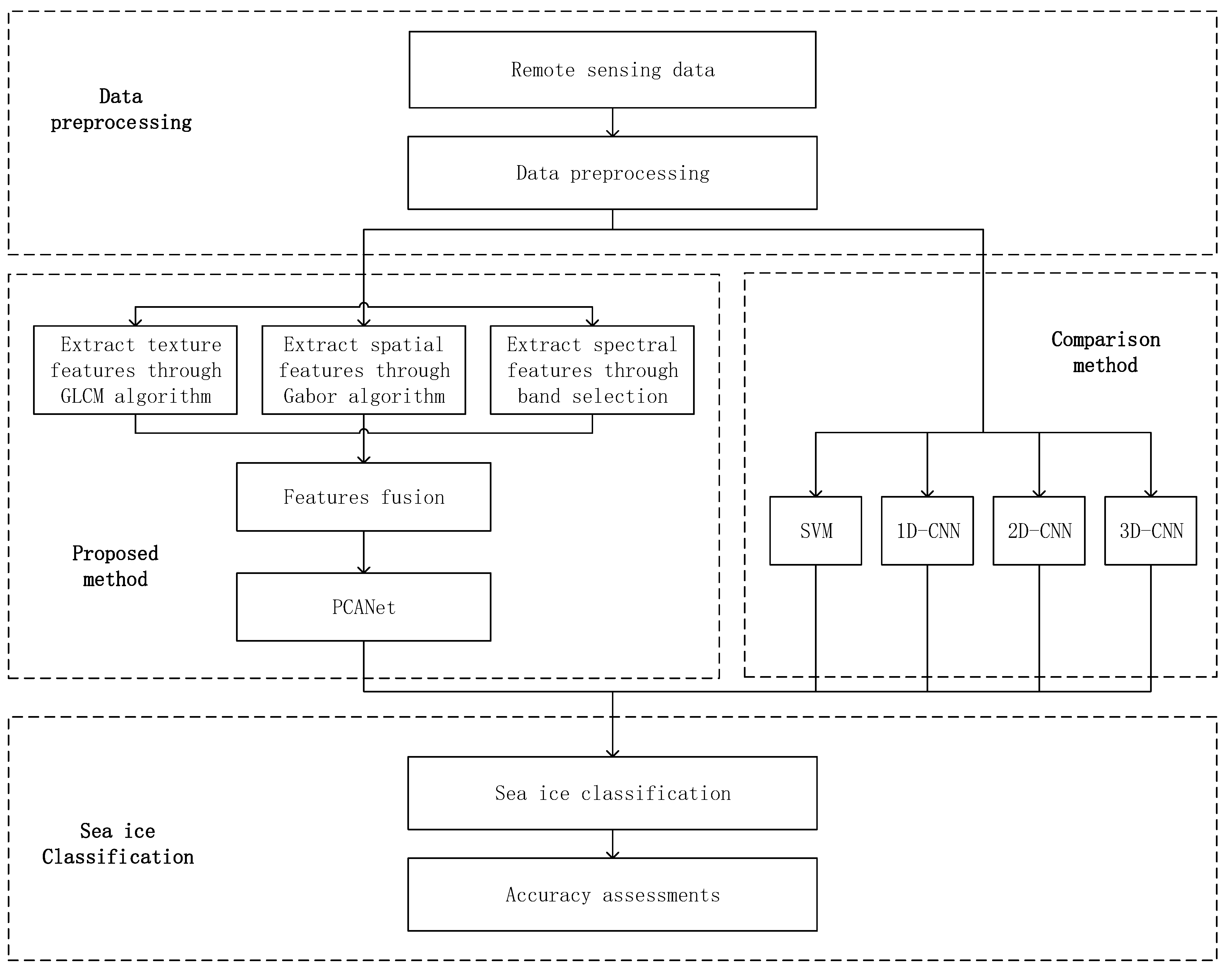
The proposed sea ice classification framework based on spectral-spatial-joint features is shown in Figure 1. It includes four main parts: the extraction of textural features based on GLCM, the extraction of spatial features based on Gabor filters, the selection of spectral features based on the band selection algorithm, and feature extraction and classification based on PCANet. Firstly, the principal component analysis is used to reduce the dimensionality, and then the GLCM and Gabor filter are used to extract textural and spatial features from hyperspectral images. The band selection algorithm and correlation analysis are used to extract the subsets of the main spectral bands from the original data. Then, the spatial and spectral feature information extracted from the two branches are fused as the input of PCANet and classified by the SVM. Finally, classification accuracy is evaluated. This algorithm is described in subsequent sections.

2.1. Texture Feature Extraction

Texture refers to small, semi-periodic, or regularly arranged patterns that exist in a certain range of images. It is one of the main features of image processing and pattern recognition. Texture is usually used to represent the uniformity, meticulousness, and roughness of images [10]. The textural features of an image reflect the attributes of the image itself and help to distinguish it.

Textural features refer to changes in of the gray value of the image, which is related to spatial statistics. The GLCM is a method of extracting textural features based on statistics. It describes the gray-level relation matrix between a pixel and adjacent pixels within a certain distance in the local or overall area of the image [22]. It reflects the joint distribution probability of pixel pairs in the image, which can be expressed as follows:

$$\begin{gathered} \mathrm{p}\left(\mathrm{i},\mathrm{j},\mathrm{d},\mathsf{\theta }\right)=\{[\left(\mathrm{x},\mathrm{y}\right),(\mathrm{x}+{\mathrm{D}}_{\mathrm{x}},\mathrm{y}+{\mathrm{D}}_{\mathrm{y}}|\mathrm{f}\left(\mathrm{x},\mathrm{y}\right)=\mathrm{i}; \\ \mathrm{f}\left(\mathrm{x}+{\mathrm{D}}_{\mathrm{x}},\mathrm{y}+{\mathrm{D}}_{\mathrm{y}}\right)=\mathrm{j};\mathrm{x}\left(\mathrm{y}\right)=0,1,2,\dots ,{\mathrm{N}}_{\mathrm{x}\left(\mathrm{y}\right)}]\} \end{gathered}$$

(1)

In Equation (1), $\mathrm{p}\left(\mathrm{i},\mathrm{j},\mathrm{d},\mathsf{\theta }\right)$ represents the times at which pixel pairs appear on the direction angle $\mathsf{\theta }$, where the gray values of pixel pairs are $\mathrm{i}$ and $\mathrm{j}$, respectively. $\mathrm{i}$, $\mathrm{j}$∈$\left\{0,1,\dots ,{\mathrm{N}}_{\mathrm{g}}-1\right\}$, where ${\mathrm{N}}_{\mathrm{g}}$ is the number of quantized gray levels, $\left(\mathrm{x},\mathrm{y}\right)$ are the relative coordinates of pixels in the image as a whole, ${\mathrm{D}}_{\mathrm{x}}$ and ${\mathrm{D}}_{\mathrm{y}}$ are horizontal and vertical offsets respectively, ${\mathrm{N}}_{\mathrm{x}}$ and ${\mathrm{N}}_{\mathrm{y}}$ are the number of columns and rows of the image respectively, $\mathrm{d}$ is the distance between pixel pairs, and $\mathsf{\theta }$ is the direction angle in the process of displacement, which is generally set as 0°, 45°, 135°, or 180° [22].

After calculating the GLCM, some statistics are usually constructed as texture classification features instead of applying the matrix directly. In this paper, eight typical texture scalars are extracted, which are the mean, variance, homogeneity, contrast, dissimilarity, entropy, angular second moment, and correlation.

2.2. Spatial Feature Extraction

The Gabor filters can effectively obtain representative frequencies and directions in the spatial domain [2]. Therefore, the establishment of a group of Gabor filters with different frequencies and directions is conducive to the accurate extraction of spatial information features. As a linear filter, the Gabor is suitable for the expression and separation of features. By extracting relevant features at different scales and in different directions in the frequency domain, it can achieve multi-scale and multi-direction features of images.

Generally speaking, the Gabor filter is defined by the Gaussian kernel function, as shown in Equation (2). Its components are divided into a real part and an imaginary part. The real part can smooth the image, while the imaginary part can be used for edge detection, as shown in Equations (3) and (4).

$$\mathrm{g}\left(\mathrm{x},\mathrm{y};\mathsf{\lambda },\mathsf{\theta },\mathsf{\psi },\mathsf{\sigma },\mathsf{\gamma }\right)=\exp \left(-\frac{{\mathrm{x}\prime }^2+{\mathsf{\gamma }}^2{\mathrm{y}\prime }^2}{2{\mathsf{\sigma }}^2}\right)\exp \left(\mathrm{i}\left(2\mathsf{\pi }\frac{\mathrm{x}\prime }{\mathsf{\lambda }}+\mathsf{\psi }\right)\right)$$

(2)

$$\mathrm{g}\left(\mathrm{x},\mathrm{y};\mathsf{\lambda },\mathsf{\theta },\mathsf{\psi },\mathsf{\sigma },\mathsf{\gamma }\right)=\exp \left(-\frac{{\mathrm{x}\prime }^2+{\mathsf{\gamma }}^2{\mathrm{y}\prime }^2}{2{\mathsf{\sigma }}^2}\right)\cos \left(2\mathsf{\pi }\frac{\mathrm{x}\prime }{\mathsf{\lambda }}+\mathsf{\psi }\right)$$

(3)

$$\mathrm{g}\left(\mathrm{x},\mathrm{y};\mathsf{\lambda },\mathsf{\theta },\mathsf{\psi },\mathsf{\sigma },\mathsf{\gamma }\right)=\exp \left(-\frac{{\mathrm{x}\prime }^2+{\mathsf{\gamma }}^2{\mathrm{y}\prime }^2}{2{\mathsf{\sigma }}^2}\right)\sin \left(2\mathsf{\pi }\frac{\mathrm{x}\prime }{\mathsf{\lambda }}+\mathsf{\psi }\right)$$

(4)

In the above equations,$\mathrm{x}\prime =\mathrm{x}\cos \mathsf{\theta }+\mathrm{y}\sin \mathsf{\theta }$,$\mathrm{y}\prime =-\mathrm{x}\sin \mathsf{\theta }+\mathrm{y}\cos \mathsf{\theta }$ is the center point of the Gaussian kernel; $\mathsf{\lambda }$ is the wavelength, which is usually not greater than one-fifth of the size of the input image;$\mathsf{\theta }$ is the direction, ranging from 0° to 360°; $\mathsf{\psi }$ is the phase offset, which mainly considers the rotation possibility of the sample and increases its robustness to rotation invariance; $\mathsf{\sigma }$ is the standard deviation of the Gaussian function; and$\mathsf{\gamma }$ represents the spatial aspect ratio, which determines the ellipticity of the shape of the Gabor function.

After the principal component analysis of the original data, a set of fixed Gabor filters was applied to extract spatial information from the images extracted by the principal component analysis after various parameters had been adjusted and optimized.

2.3. Band Selection

Generally speaking, a reduction in the dimensionality of hyperspectral data can be achieved by feature extraction or feature selection (band selection). Band selection can effectively reduce the amount of redundant information without affecting the original content by selecting a group of representative bands in the hyperspectral image [23]. This paper adopts a band selection algorithm based on a hybrid strategy. The purpose of this algorithm is to select the best band combinations that provide a large amount of information, less relevance, and strong category separability. The main idea is to find the best band division using the evaluation criterion function, and then evaluate all bands using the mixed strategy of clustering and sorting. Finally, the bands with the highest level in each division are used to form the final best band combination [24].

In this paper, two objective functions, the Normalized Cut and Top-Rank Cut, are used to divide bands. The smaller the value of the former, the higher the intra-group correlation and the lower the inter-group correlation of each band combination. The smaller the value of the latter, the lower the overall correlation. Both of these partitioning functions are beneficial for subsequent sorting selection. In the mixed strategy, we adopt the maximum variance principal component analysis (MVPCA), information entropy (IE) based on sorting and the enhanced rapid density peak clustering (E-FDPC) based on clustering.

2.4. PCANet

Compared with previous convolution neural networks, the PCANet deep learning framework has strong competitiveness in terms of feature extraction. It can be used to train a simple network to learn data and learn low-level features from the data. These low-level features constitute high-level features with abstract meaning and invariance, which is beneficial for image classification, target detection, and other tasks [25]. In hyperspectral image classification, PCANet can choose the adaptive convolution filter group as the basic principal component analysis filter, and hash binarization mapping and block histogram enhance feature separation and reduce feature dimension, respectively [21]. At the same time, the spatial pyramid is used to extract the invariant features, and finally, the SVM classifier is used to output the classification results. The specific network structure includes PCA convolution layers, a nonlinear processing layer (NP layer), and a feature pooling layer (FP layer), as shown in Figure 2.

Assuming that our input training set ${\left\{{\mathrm{I}}_{\mathrm{i}}\right\}}_{\mathrm{i}=1}^{\mathrm{N}}$ contains $\mathrm{N}$ images of size $\mathrm{m}\times \mathrm{n}$, the filter size in all convolutional layers is ${\mathrm{k}}_1\times {\mathrm{k}}_2$. We need to learn the principal component analysis filter from ${\left\{{\mathrm{I}}_{\mathrm{i}}\right\}}_{\mathrm{i}=1}^{\mathrm{N}}$, and the following text introduces the proposed architecture.

2.4.1. The First PCA Convolution Layer

First, each pixel in the input image ${\mathrm{I}}_{\mathrm{i}}$ is sampled with a ${\mathrm{k}}_1\times {\mathrm{k}}_2$ block, and then these sample blocks are cascaded to get an $\tilde{\mathrm{m}}\times \tilde{\mathrm{n}}$ block. The sample block of image ${\mathrm{I}}_{\mathrm{i}}$ is expressed as $\left[{\mathrm{x}}_{\mathrm{i},1},{\mathrm{x}}_{\mathrm{i},2},\dots ,{\mathrm{x}}_{\mathrm{i},\tilde{\mathrm{m}}\tilde{\mathrm{n}}}\right]\in {ℝ}^{{\mathrm{k}}_1{\mathrm{k}}_2}$, where $\tilde{\mathrm{m}}=\mathrm{m}-{\mathrm{k}}_1/2$, $\tilde{\mathrm{n}}=\mathrm{n}-{\mathrm{k}}_2/2$. Then, the sample block is de-zeroed and averaged to obtain ${\overline{\mathrm{X}}}_{\mathrm{i}}=\left[{\overline{\mathrm{x}}}_{\mathrm{i},1},{\overline{\mathrm{x}}}_{\mathrm{i},2},\dots ,{\overline{\mathrm{x}}}_{\mathrm{i},\tilde{\mathrm{m}}\tilde{\mathrm{n}}}\right]\in {ℝ}^{{\mathrm{k}}_1{\mathrm{k}}_2}$, where ${\overline{\mathrm{x}}}_{\mathrm{i},\mathrm{j}}={\mathrm{x}}_{\mathrm{i},\mathrm{j}}-\frac{{\mathrm{x}}_{\mathrm{i},\mathrm{j}}}{{\mathrm{k}}_1{\mathrm{k}}_2}$ is a sample block with the average value removed. Then, the same processing is done on the rest of the images. Finally, the training sample matrix is obtained, as shown in Equation (5). The PCA algorithm minimizes the reconstruction error by looking for a series of orthonormal matrices. We assume that the number of filters in the $\mathrm{i}-\mathrm{th}$ layer is ${\mathrm{L}}_{\mathrm{i}}$, so the reconstruction error can be expressed by Equation (6). Similarly to the classic principal component analysis algorithm, the first $\mathrm{n}$ eigenvectors of the covariance matrix of matrix $\mathrm{X}$ need to be obtained, so the representation of the corresponding filter is shown in Equation (7), where the $\mathrm{mat}$ function is used to transform the vector into a matrix, and ${\mathrm{q}}_{\mathrm{l}}$ represents the $\mathrm{l}-\mathrm{th}$ principal eigenvector. The output of the first layer is shown by Equation (8), where $*$ represents convolution operation and ${\mathrm{I}}_{\mathrm{i}}$ is the $\mathrm{i}-\mathrm{th}$ input image.

$$\mathrm{X}=\left[{\overline{\mathrm{X}}}_1,{\overline{\mathrm{X}}}_2,\dots ,{\overline{\mathrm{X}}}_{\mathrm{N}}\right]\in {ℝ}^{{\mathrm{k}}_1{\mathrm{k}}_2\times \mathrm{N}\tilde{\mathrm{m}}\tilde{\mathrm{n}}}$$

(5)

$$\min \parallel \mathrm{X}-{\mathrm{VV}}^{\mathrm{T}}\mathrm{X}{\parallel }_{\mathrm{F}}^2,\mathrm{s.t.}{\mathrm{V}}^{\mathrm{T}}\mathrm{V}={\mathrm{I}}_{\mathrm{L}1},\mathrm{V}\in {ℝ}^{{\mathrm{k}}_1{\mathrm{k}}_2\times {\mathrm{L}}_1}$$

(6)

$${\mathrm{W}}_{\mathrm{l}}^1={\mathrm{mat}}_{{\mathrm{k}}_1{\mathrm{k}}_2}\left({\mathrm{q}}_{\mathrm{l}}\left({\mathrm{XX}}^{\mathrm{T}}\right)\right)\in {ℝ}^{{\mathrm{k}}_1\times {\mathrm{k}}_2},\mathrm{l}=1,2,\dots ,{\mathrm{L}}_1$$

(7)

$${\mathrm{C}}_{\mathrm{i}}^{\mathrm{l}}={\mathrm{I}}_{\mathrm{i}}{*\mathrm{W}}_{\mathrm{l}}^1,\mathrm{i}=1,2,\dots ,\mathrm{N}$$

(8)

2.4.2. The nth PCA Convolution Layer

The subsequent convolution layer process is same that for as the first layer. First, the output ${\mathrm{C}}_{\mathrm{i}}^{\mathrm{l}}$ of the previous layer is calculated. Then, the sample is zeroed to the edge to ensure it is the same size as the original image. The output is subjected to operations such as block sampling, cascading, and de-averaging. Similarly, the feature vector and output of the $\mathrm{n}-\mathrm{th}$ layer are obtained. It is worth noting that since the first layer has ${\mathrm{L}}_1$ filters, the first layer generates ${\mathrm{L}}_1$ output matrices, and the second layer generates ${\mathrm{L}}_2$ outputs for each output by the first layer, which is accumulated layer by layer. For each sample, the $\mathrm{n}-\mathrm{order}$ PCANet generates ${\displaystyle \prod }_{\mathrm{a}=1}^{\mathrm{n}}{\mathrm{L}}_{\mathrm{a}}$ output feature matrices, and the final output feature is expressed as shown in Equation (9). Thus, it can be seen that the individual convolutional layers of the PCANet are structurally similar, which facilitates the construction of the multi-layer deep network.

$${\mathrm{O}}_{\mathrm{i}}^{\mathrm{l}}={\left\{{\mathrm{C}}_{\mathrm{i}}^{\mathrm{l}}{*\mathrm{W}}_{\mathrm{l}}^{\mathrm{n}}\right\}}_{\mathrm{l}}^{{\mathrm{L}}_{\mathrm{n}}}$$

(9)

2.4.3. Nonlinear Processing Layer

In previous work, we obtained the features through the convolution layer and then used the hash algorithm to perform nonlinear processing on the output of the previous layer. The specific operation used is as follows: binary hash encoding is carried out on each output to reset the pixels and index to enhance the separation between different features. ${\mathrm{L}}_{\mathrm{n}}$ images form a vector of length ${\mathrm{L}}_{\mathrm{n}}$, and each vector is converted to a decimal as the output of the non-linear processing layer. The function is shown below:

$${\mathrm{T}}_{\mathrm{i}}^{\mathrm{l}}={\displaystyle {{\displaystyle \sum }}_{\mathrm{l}=\mathrm{C}}^{{\mathrm{L}}_{\mathrm{n}}}}{2}^{\mathrm{l}-1}\mathrm{H}\left({\mathrm{C}}_{\mathrm{i}}^{\mathrm{l}}{*\mathrm{W}}_{\mathrm{l}}^{\mathrm{n}}\right)$$

(10)

2.4.4. Feature Pooling Layer

After the nonlinear processing layer, each output matrix is divided into $\mathrm{B}$ blocks, and the histogram information of the decimal values in each block is calculated and cascaded into a vector to obtain the final block expansion histogram features, as shown in Equation (11). Histogram features add some stability to the variation in the features extracted by PCANet while reducing the feature dimension [26]. In order to improve the multi-scale property of the spatial features, a spatial pyramid module is added after the block histogram to give the features a better distinguishing ability. Finally, the SVM classifier is selected to get the final output.

$${\mathrm{f}}_{\mathrm{i}}={[\mathrm{Bhist}\left({\mathrm{T}}_{\mathrm{i}}^{\mathrm{l}}\right),\dots ,\mathrm{Bhist}\left({\mathrm{T}}_{\mathrm{i}}^{{\mathrm{L}}_{\mathrm{n}-1}}\right)]}^{\mathrm{T}}\in {ℝ}^{{(2^{{\mathrm{L}}_{\mathrm{n}}})}^{{\mathrm{L}}_{\mathrm{n}-1}\mathrm{B}}}$$

(11)

2.5. Algorithm Process Description

After describing the above framework, the specific implementation process for the Algorithm 1 used in this paper is as follows:

Algorithm 1. The Proposed Algorithm Process.

Begin Input: the labeled sample set with a size of $\mathrm{M}\times \mathrm{N}\times \mathrm{B}$, where M × N is the size of the input image and B is the number of bands. A. Feature extraction and fusion (1) Based on the band selection algorithm, the original band is selected to obtain the optimal band combination after selection, and the spectral features Fs are extracted; (2) The primary component analysis algorithm is used to process the original data, and the first principal component PC is obtained; (3) Using the gray-scale co-occurrence matrix algorithm, the gray-scale co-occurrence matrix of the sliding window based on the principal component PC in each direction at angle θ and step d is calculated, and the texture eigenvalue of the center pixel is obtained; (4) Repeat (2) until the principal component area is completely covered by the sliding window; (5) The texture features at each direction angle θ are averaged to obtain the final texture feature matrix; (6) Repeat (4) until the five texture features are obtained and the extraction of texture features Fg1 has been completed; (7) According to the Gabor algorithm, set a group of filter banks with scale s and direction θ; (8) Based on the results of (1), the results for the principal component PC based on Gabor filters at various scales and directions are calculated to obtain the final spatial feature information; (9) Repeat (8) until sixteen spatial features have been obtained to complete the extraction of spatial features Fg2; (10) Fuse the features of (1), (6), and (9) to complete the extraction and fusion of features. B. PCANet (1) Randomly select training samples with a certain training testing ratio and input them into the pre-established PCANet network; (2) The first principal component analysis filter is used to obtain the high-level abstract features, and the filter parameters ${\mathrm{W}}_{\mathrm{l}}^{\mathrm{i}}$ are learned to calculate the first-layer convolution output ${\mathrm{C}}_{\mathrm{i}}^{\mathrm{l}}$; (3) The output in (2) is taken as the input and (2) is repeated until all PCA filter layers have been calculated, and the output of the last layer ${\mathrm{O}}_{\mathrm{i}}^{\mathrm{l}}$ has been obtained; (4) The separation between features is enhanced by hashing binarization, and ${\mathrm{O}}_{\mathrm{i}}^{\mathrm{l}}$ is hash-encoded and converted to a decimal to obtain ${\mathrm{T}}_{\mathrm{i}}^{\mathrm{l}}$; (5) The feature dimension is reduced by the block histogram, and the statistical histogram information is cascaded to get the final block extended histogram feature fi, and then the spatial pyramid is used to generate multi-scale spatial features; (6) The SVM classifier is used for classification. Output: Confusion matrix, Overall accuracy (OA), Kappa value. End

3. Experimental Results and Discussion

In order to verify the effectiveness of the method proposed in this paper, we used two hyperspectral remote sensing sea ice data sets in the experiment: images of Bohai Bay and Baffin Bay were captured by Earth Observation Satellite-1 (EO-1). We compared the proposed algorithm with four other algorithms: SVM [10], one-dimensional convolutional neural network (1D-CNN), two-dimensional convolutional neural network (2D-CNN), three-dimensional convolutional neural network (3D-CNN), and gray-level co-occurrence matrix convolutional neural network (GLCM-CNN) [22]. All classification algorithms evaluated the experimental results in terms of the overall accuracy (OA) and the kappa statistic. Each algorithm ran the experiments 10 times with different initial random training samples. The experimental environment used was an Intel(R) Core(TM) i5-6500CPU with 3.20 GHz and 20 GB of installed memory.

3.1. Experiment in Bohai Bay

3.1.1. Data Description

The first data set used in the experiment was a cloud-free Hyperion image of the Bohai Bay area taken on 23 January 2008. The original size of the image was 7061 pixels × 2001 pixels, and the spatial resolution was 30 m. After removing the low SNR and water absorption bands from the original 242 bands, 176 bands were selected for analysis. A scene covered by sea ice with a size of 442 pixels × 212 pixels was cropped from the original image and used as the experimental area. According to the spectral curve, the experimental area could be roughly divided into four categories: white ice, gray-white ice, gray ice, and sea water. As shown in Figure 3a, the experimental area was a false-color image composed of bands R: 30, G: 25, and B: 18, and the corresponding labeled samples are shown in Figure 3b. The labeled samples were randomly divided into training samples and test samples at a ratio of 1:9, as shown in

Table 1. Number of training samples (pixels) and testing samples (pixels) in each class for the Bohai Bay data set.

Class	Training	Test
White ice	12	111
Gray_White ice	31	278
Gray ice	30	267
Sea water	20	172
Total	93	828

.

3.1.2. Experimental Setup

Generally speaking, the hyperspectral classification algorithm which only uses spectral features does not fully utilize the spatial information, which limits the further improvement of classification accuracy. Especially for spectral information relatively similar within classes, making full use of spatial information can further improve the classification accuracy [25]. In this experiment, we studied different spatial feature extraction methods and combined spatial features and spectral features.

Although the GLCM provides information on the gray-level direction, interval, and variation in the amplitude of the image, it cannot directly determine the distinguishing texture. In addition, the highly correlated components in texture features extracted by GLCM need to be removed through a correlation analysis [23]. As shown in

Table 2. Correlation matrix for eight texture components in the Bohai Bay data set.

	Mea	Var	Hom	Con	Dis	Ent	ASM	Cor
Mea	1	0.0893	−0.7219	0.0523	0.3383	0.8692	−0.7839	−0.4531
Var	-	1	−0.1605	0.7862	0.7123	0.1381	−0.1275	−0.0426
Hom	-	-	1	−0.1728	−0.4961	−0.8133	0.8887	0.5450
Com	-	-	-	1	0.8911	0.1305	−0.1236	−0.0544
Dis	-	-	-	-	1	0.4382	−0.3896	−0.1966
Ent	-	-	-	-	-	1	−0.9201	−0.5529
ASM	-	-	-	-	-	-	1	0.6577
Cor	-	-	-	-	-	-	-	1
AAC	0.5385	0.3821	0.5998	0.4014	0.5578	0.6078	0.6114	0.4378

(Mea: Mean, Var: Variance, Hom: Homogeneity, Con: Contrast, Dis: Dissimilarity, Ent: Entropy, ASM: Angular second moment, Cor: Correlation, AAC: Average absolute correlation).

, the correlation analysis was conducted on eight texture components in the Bohai Bay data. When the absolute value of the correlation coefficient of two texture features was greater than 0.8, we classified them as highly correlated. In this case, texture features with smaller average absolute correlation values were selected for further study. Based on the correlation matrix, five texture components with low similarity were finally retained: the mean, variance, homogeneity, contrast, and correlation.

In order to extract more abundant spatial features, we studied the multi-direction and multi-scale Gabor filters and then selected suitable Gabor filters through parameter tuning. Finally, we used four filter scale sizes of 7, 9, 11, and 13 in the experiment and four directions, θ = 0, π/4, π/2, and 3π/4, were determined for each scale.

We conducted a principal component analysis on the original image and used the five texture features extracted by the GLCM and the 16 spatial features extracted by the Gabor filter. The spectral features were combined after band selection and finally input into the network model for training and classification. The model proposed in reference [5] has a simple structure and is easy to train. On this basis, we adjusted the parameters and optimized the structure. The structure of the network model is shown in

Table 3. Network structure of the Bohai Bay data set.

Layer	PCA1st	PCA2nd	NP	FP
PatchSize	(5,5)	(5,5)	-	-
NumFilters	8	8	-	-
HistBlockSize	-	-	(5,5)	-
BlkOverLapRatio	-	-	0.5	-
Pyramid	-	-	-	(1,2,4)

(PCA1st: PCANet first convolution, PCA2nd: PCANet second convolution, NP: nonlinear layer (hash binarization), FP: feature pooling layer (histogram quantization and spatial pyramid pooling), PatchSize: batch size, NumFilters: the number of filters, HistBlockSize: the size of histogram block, BlkOverLapRatio: overlap rate, Pyramid: spatial pyramid pooling).

. The model contains an input layer, two convolution layers, a nonlinear layer, a feature pooling layer, and an output layer. The data input size was 8 × 8, and 93 samples were randomly input in each training session. The average of 10 rounds of training was taken as the final evaluation result.

3.1.3. Experimental Results and Discussion

The classification results for the Bohai Bay data are shown in

Table 4. Combination classification results (%) of spectral features and spatial features of the Bohai Bay dataset.

BN	${\mathrm{F}}_{\mathrm{s}}$	${\mathrm{F}}_{\mathrm{s}}+{\mathrm{F}}_{\mathrm{g}1}$	${\mathrm{F}}_{\mathrm{s}}+{\mathrm{F}}_{\mathrm{g}2}$	${\mathrm{F}}_{\mathrm{s}}+{\mathrm{F}}_{\mathrm{g}1}+{\mathrm{F}}_{\mathrm{g}2}$
	Accu(%)
30	93.21	93.04	91.75	94.15
All bands	91.63	91.95	91.14	92.54

(Accu: classification accuracy, BN: number of bands, ${\mathrm{F}}_{\mathrm{s}}$: using only spectral features, ${\mathrm{F}}_{\mathrm{s}}+{\mathrm{F}}_{\mathrm{g}1}$: combining spectral features and texture features extracted by GLCM, F_s + F_g2: combining spectral features and spatial features extracted by Gabor filtering, ${\mathrm{F}}_{\mathrm{s}}+{\mathrm{F}}_{\mathrm{g}1}+{\mathrm{F}}_{\mathrm{g}2}$: combining the above three features).

. In the experiment, after band selection, the input size when only spectral features and textural features was 6 × 6, and the input size when only spatial features were used by Gabor was 7 × 7. The input size when all of the above were combined was 8 × 8. The input size of the original spectral features and the two spatial features was 14 × 14 while that of the fusion method was 15 × 15. It can be seen from Table 4 that compared with other combinations, the combination of spectral features after band selection and two spatial features achieved the best classification result, with an average accuracy of 94.15%. The classification accuracy after band selection was 2.51% higher than that using the whole band, which indicates that removing highly correlated and redundant bands can effectively improve the classification accuracy. In terms of feature combinations, the fusion of single spatial features and spectral features did not achieve a great improvement, while the fusion of two spatial features and spectral features improved the result by 0.94%.

Table 5. Classification results (%) of the Bohai Bay data set.

	SVM	1D-CNN	2D-CNN	3D-CNN	GLCM-CNN	Proposed
White ice	73.87	77.48	81.89	83.78	87.68	88.28
Gray_White ice	86.25	83.45	86.69	90.53	93.17	95.68
Gray ice	88.76	89.14	92.13	93.63	95.63	96.25
Sea water	94.76	95.35	96.51	94.18	95.35	96.34
OA	85.21	86.38	89.21	90.14	92.05	94.15
Kappa × 100	81.99	83.51	86.85	87.54	89.24	92.46

shows the classification results for the Bohai Bay dataset based on different classification methods. In general, the classification accuracy of the SVM algorithm, which is a shallow learning method, was relatively low, only 85.21%. Although the one-dimensional convolutional neural network, which only uses spectral features, was found to be better than the SVM, neither of them utilize spatial features. The classification accuracy of the proposed method in this paper was 4.94% and 4.01% higher than that of 2D-CNN and 3D-CNN, respectively, both of which use spatial features. This shows that fully mining spatial features and performing fusion on spectral and spatial features can effectively improve the sea ice classification accuracy. The GLCM-CNN produced more accurate results than the 3D-CNN, which reflects the effectiveness of the texture information extracted by the GLCM. The classification accuracy of the proposed method improved by 2.1% compared with that of GLCM-CNN, which indicates that compared with the convolutional neural network, the proposed PCANet network can choose the data adaptive convolution filter as the principal component analysis filter and enhance the separation of features through hash binarization mapping and the block histogram, which is a better feature extraction method. It can obtain a better classification effect by using fewer training samples. In sea water and three types of sea ice, this method is advantageous for the classification of sea ice. Compared with 3D-CNN and GLCM-CNN, the classification accuracy of white ice was found to increase by 4.5% and 0.6%, respectively, and that of gray-white ice and gray ice increased by 5.15%, 2.51%, 2.62%, and 0.62%, respectively.

In addition, result maps are shown in Figure 4. The classification result maps show that the method is an advantageous one for classifying two intermediate seawater categories and three sea ice categories as it can distinguish the boundary between gray ice and gray-white ice more clearly. The proposed method effectively eliminates the noise points and makes the distinction between different types of edge regions more accurate.

3.2. Experiment in Baffin Bay

3.2.1. Data Description

The second dataset used in the experiment was a cloud-free Hyperion image of Baffin Bay area taken on 12 April 2014. The original size of the image was 2395 pixels × 1769 pixels, and it had a spatial resolution of 30 m. Similar to the Bohai Bay dataset, we selected 176 bands out of the original 242 bands for subsequent analysis, and cropped 212 pixels × 300 pixels from the original image as the experimental area, which was divided into three main categories: white ice, gray ice, and sea water. As shown in Figure 5a, this was a false-color image of the experimental area composed of three bands (R: 175, G: 168, and B: 150). The corresponding labeled samples are shown in Figure 5b, and the labeled samples were randomly divided into training samples and test samples at a ratio of 1:9, as shown in

Table 6. Number of training samples (pixels) and testing samples (pixels) in each class for the Baffin Bay data set.

Class	Training	Test
White ice	60	524
Gray ice	42	348
Sea water	21	180
Total	123	1052

.

3.2.2. Experimental Setup

Similar to the Bohai Bay dataset, for the Baffin Bay dataset,

Table 7. Correlation matrix for eight texture components in the Baffin Bay data set.

	Mea	Var	Hom	Con	Dis	Ent	ASM	Cor
Mea	1	−0.1075	0.4866	−0.1019	−0.1422	−0.1542	0.4296	0.2217
Var	-	1	−0.4952	0.7873	0.6888	0.4711	−0.3628	0.1710
Hom	-	-	1	−0.5937	−0.8044	−0.7052	0.8177	0.0940
Com	-	-	-	1	0.8819	0.4783	−0.3705	0.1354
Dis	-	-	-	-	1	0.7336	−0.6008	0.1130
Ent	-	-	-	-	-	1	−0.8766	−0.0823
ASM	-	-	-	-	-	-	1	0.3009
Cor	-	-	-	-	-	-	-	1
AAC	0.3305	0.5105	0.6246	0.5436	0.6206	0.5627	0.5949	0.2648

(Mea: Mean, Var: Variance, Hom: Homogeneity, Con: Contrast, Dis: Dissimilarity, Ent: Entropy, ASM: Angular second moment, Cor: Correlation, AAC: Average absolute correlation).

shows the correlation matrix used to extract the corresponding texture features based on the GLCM, and feature exclusion was conducted according to the correlation value. Because the level of dissimilarity was highly correlated with the level of homogeneity and contrast, and because the level of homogeneity had greater similarity with the angular second moment, the contrast feature was retained. Similarly, the angular second moment and entropy had high similarity, so the texture feature of the angular second moment was excluded. The five remaining texture components were the mean, variance, contrast, entropy, and correlation.

The parameters used by the Gabor filter to extract spatial features were similar to those used for the Bohai Bay dataset, but the difference was that the four scales of the filter were set as 5, 7, 9, and 11 respectively. After analyzing the original spectral information with the same band selection algorithm, the extracted spatial features were combined into the network, and the structure of network was as shown in

Table 8. Network structure of the Baffin Bay data set.

Layer	PCA1st	PCA2nd	PCA3rd	NP	FP
PatchSize	(3,3)	(3,3)	(3,3)	-	-
NumFilters	8	8	8	-	-
HistBlockSize	-	-		(5,5)	-
BlkOverLapRatio	-	-		0.5	-
Pyramid	-	-		-	(1,2,4)

(PCA1st: PCANet first convolution, PCA2nd: PCANet second convolution, PCA3rd: PCANet third convolution, NP: nonlinear layer (hash binarization), FP: feature pooling layer (histogram quantization and spatial pyramid pooling), PatchSize: batch size, NumFilters: the number of filters, HistBlockSize: the size of histogram block, BlkOverLapRatio: overlap rate, Pyramid: spatial pyramid pooling).

. The model consists of an input layer, three convolution layers, a nonlinear layer, a feature pooling layer, and an output layer. The size of the input data was 8 × 8, and 123 samples were randomly input for each training session. Similarly, the average of 10 rounds of training was taken as the final evaluation result.

3.2.3. Experimental Results and Discussion

The classification results of the Baffin Bay data are shown in

Table 9. Combination classification results (%) of spectral features and spatial features of the Baffin Bay dataset.

BN	${\mathrm{F}}_{\mathrm{s}}$	${\mathrm{F}}_{\mathrm{s}}\times +\times {\mathrm{F}}_{\mathrm{g}1}$	${\mathrm{F}}_{\mathrm{s}}\times +\times {\mathrm{F}}_{\mathrm{g}2}$	${\mathrm{F}}_{\mathrm{s}}\times +\times {\mathrm{F}}_{\mathrm{g}1}\times +\times {\mathrm{F}}_{\mathrm{g}2}$
	Accu. (%)
30	93.87	96.65	95.63	96.86
All bands	91.57	93.36	93.69	94.26

(Accu: classification accuracy, BN: number of bands, ${\mathrm{F}}_{\mathrm{s}}$: using only spectral features, F_s + F_g1: combining spectral features and texture features extracted by GLCM, F_s + F_g2: combining spectral features and spatial features extracted by Gabor filtering, ${\mathrm{F}}_{\mathrm{s}}+{\mathrm{F}}_{\mathrm{g}1}+{\mathrm{F}}_{\mathrm{g}2}$: combining the above three features).

and

Table 10. Classification results (%) of the Baffin Bay data set.

	SVM	1D-CNN	2D-CNN	3D-CNN	GLCM-CNN	Proposed
White ice	97.14	97.52	99.43	99.62	99.81	99.81
Gray ice	78.74	79.46	86.49	90.52	90.05	92.59
Sea water	92.11	92.00	93.56	94.11	94.08	97.35
OA (%)	90.70	90.19	93.40	94.08	95.01	96.86
Kappa × 100	85.41	86.27	89.53	92.65	92.76	95.12

. For the feature combination results, the input size was the same as that of the Bohai Bay dataset. It can be seen from Table 9 that the classification accuracy of the method in this paper was the highest. The overall classification effect of the band selection method was better than that of the full-band method, which indicates that the existence of redundant and highly correlated bands had a greater impact on the results. When the number of bands was the same, the extraction of spatial and texture features enriched the information contained in the samples, which improved the final classification accuracy by 2–3%. In addition, the spatial and texture information extracted by combining the two methods was found to be more advantageous for classification than that extracted by using spectral information alone. The classification accuracy of the former was found to be 2.99% higher than that of the latter.

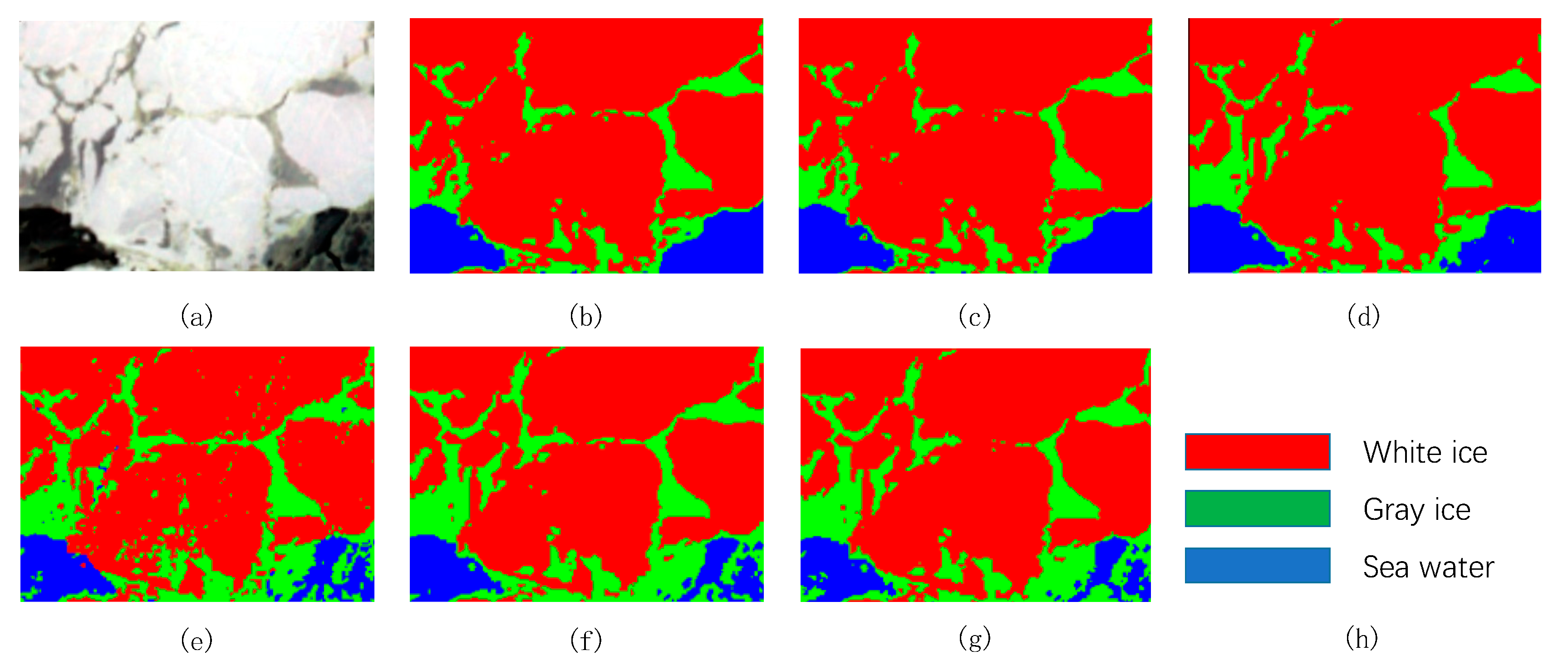
As shown in Table 10, the classification accuracy for gray ice in the compared methods is relatively low, and it is difficult to distinguish gray ice using the spectral features contained in the SVM and 1D-CNN. However, in the method proposed in this paper, the classification of gray ice by spatial features is improved. Compared with other algorithms, the proposed method has the highest overall classification accuracy (OA = 96.86%): 6.16%, 6.67%, 3.46%, 2.78%, and 1.85% higher than that of SVM (90.70%), 1D-CNN (90.19%), 2D-CNN (93.40%) 3D-CNN (94.08%), and GLCM-CNN (95.01%), respectively. The classification result images are shown in Figure 6, where the visual classification result of the proposed method at the category boundaries was found to be more precise. For example, as can be seen from the lower right corner of the experimental area, for the intermediate category (gray ice), the proposed method better distinguished gray ice from sea water. This shows that the proposed method can effectively extract feature information from samples. Compared with the convolutional neural network, the proposed method can learn the low-level features from the data, and these low-level features constitute more abstract high-level features, which are suitable for the classification of hyperspectral sea ice images.

3.3. Parameter Influence Analysis

It can be seen from the experiment that in the classification of hyperspectral sea ice images, various parameters and the number of bands in the deep learning network affect the final classification accuracy. This section details our analysis of the experimental results in which we changed the number of network layers, the number of filters, the size of the filters, and the number of bands in the model. In addition, the parameters of the feature pooling layer were fixed in this experiment. The size of the histogram blocks for the Bohai Bay data and Baffin Bay data were 7 × 7 and 5 × 5 respectively, and the sizes of the spatial pyramid pools were set to 1 × 1, 2 × 2, and 4 × 4.

3.3.1. The Number of PCA Layers

As can be seen from Figure 2, the network used in this paper has multiple layers, that is, multiple PCA processing stages, which can extract image features several times. We analyzed the number of network layers in the two data sets, and the experimental results are shown in Figure 7. The results show that for Bohai Bay, the classification accuracy generally decreases as the number of network layers increase. For Baffin Bay, the best classification accuracy was achieved when the number of network layers was 3, and then it decreased. In general, a lot of training layers should not be used in the PCA. Based on the data, setting 2 or 3 network layers can improve the classification accuracy.

3.3.2. The Number of Filters

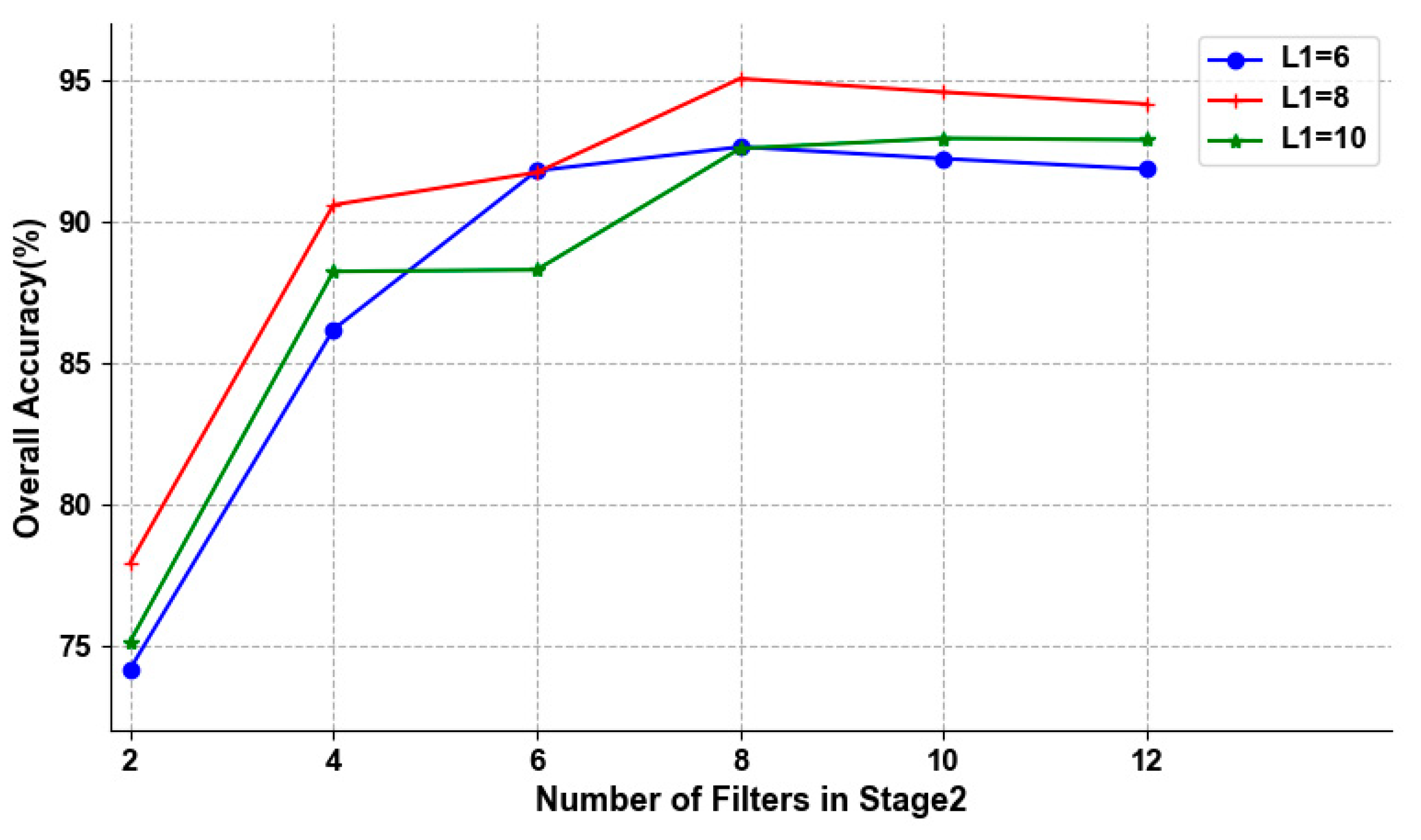
The key characteristic of the method proposed in this paper is that each image needs to be convoluted through the filter generated by the feature vector, so the number of filters will inevitably have an impact on the classification accuracy. We chose to use the Bohai Bay dataset with a two-layer PCA network for the experiment. The number of filters in the first layer (L1) was controlled as a fixed value each time, and the experimental results are shown in Figure 8. In general, as the number of filters in the second layer network (L2) increased, the classification accuracy showed an obvious increasing trend. When L1 = L2 = 8, the highest level of accuracy reached was 95.43%, and then a downward trend began. Therefore, the number of two-layer filters selected was L1 = L2 = 8 in this paper.

3.3.3. The Size of Filters

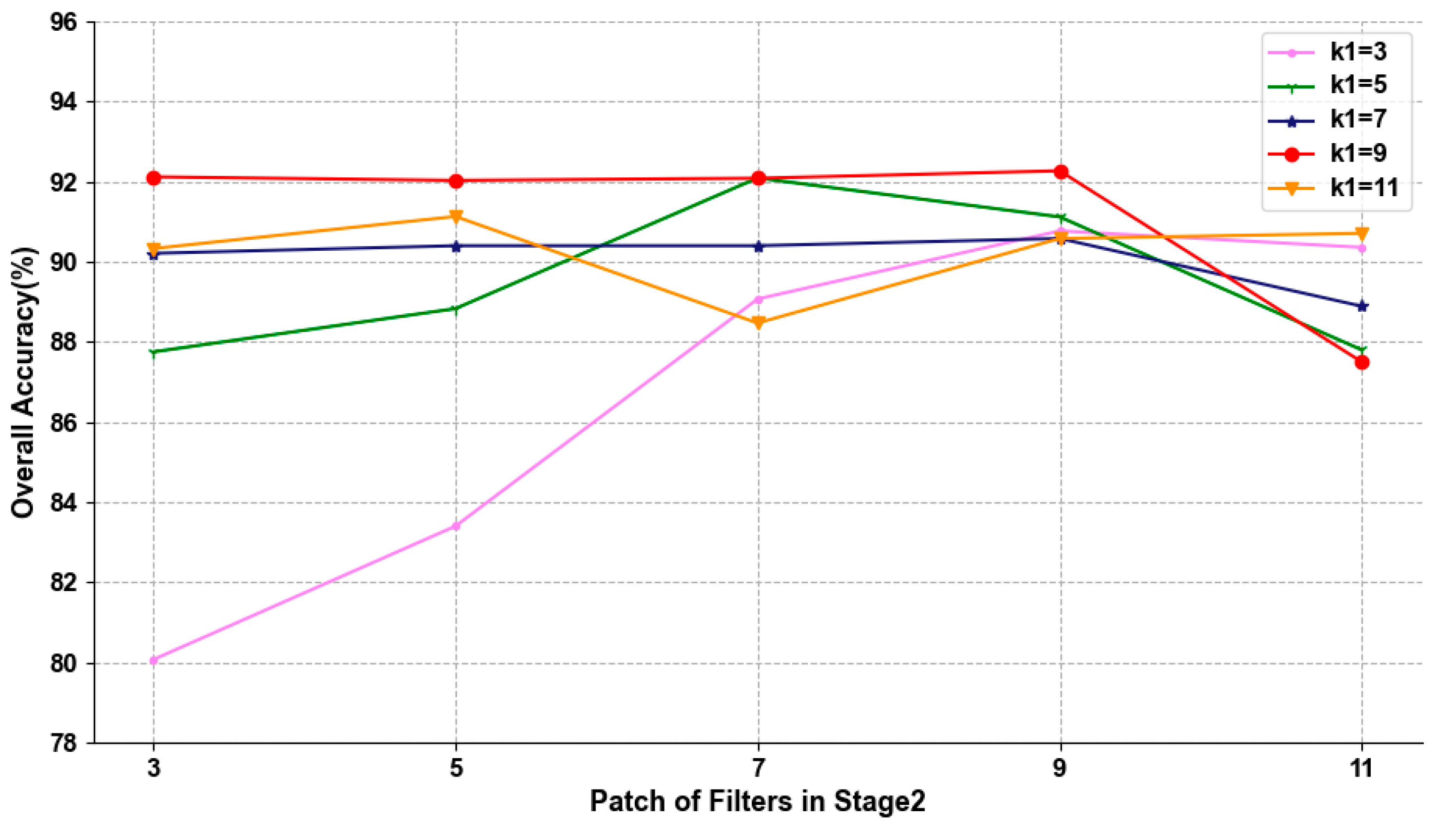
In the training of a deep learning model, the influence of the filter size on the classification results cannot be ignored. By changing the filter size of each layer, the influence of the filter on the classification accuracy was further studied. Considering the size of the input, we changed the size of the filter of the first layer (k1) in the Bohai Bay dataset from 3 to 11 at an interval of 2, and then we changed the size of the filter of the second layer (k2) for the experiment. Figure 9 shows that when k1 was fixed and k2 was changed, the classification accuracy changed slightly. When k1 = 3 or 5, the classification accuracy increased as k2 increased and tended to be stable when k2 = 7 or 9. When k1 = 7, 9, or 11, the overall trend was similar to the increase of k2. It tended to be flat at first and then decreased. In general, for this experimental dataset, the size of filter needed to be equal to half of the input, and the filter size of the first layer needed to be bigger than the second layer, but the interval could not be too large. If the filter was too small, there was a possibility that it would not contain enough information, and if the filter was too large, it could too much redundant and irrelevant information, both of which would lead to a low classification accuracy.

It is worth noting that considering the three-layered structure of Baffin Bay, we set the size of the filter of the second layer to be same as that of the first layer, and we changed the size of k3 and other settings to be similar to those of the Bohai Bay dataset. The experimental results are shown in Figure 10. It can be seen from the figure that when k1 = k2 = 3, 5, 7, and 9, the classification accuracy first increased and then decreased as k3 increased. When the size of the filter was 11, the overall trend was downward. The results show the same characteristics and conclusions as those of the experiment in Bohai Bay. The filter size of the layers needed to be half of the input, and the interval of each layer could not be too large. In addition, because the filter extracts the local features of the image, the size of the filter could not be too large as this would increase the number of redundant features, introducing more errors into the classification and leading to a reduction in the classification accuracy.

3.3.4. The Number of Bands

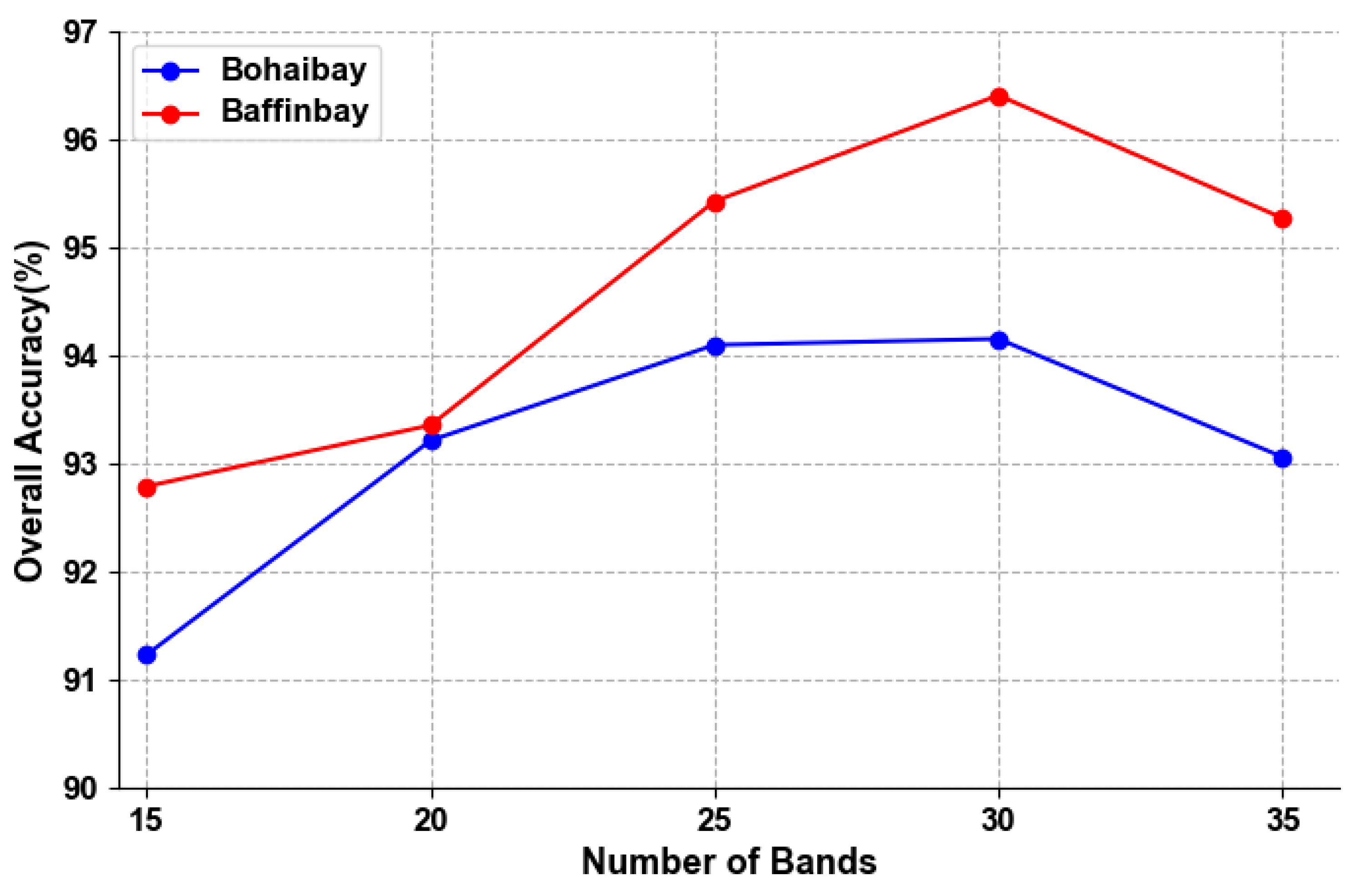
In order to retain bands with rich information and low correlation as much as possible, we first needed to determine the number of bands and then select the corresponding number of bands through a correlation analysis. Finally, we determined the band combination according to the results. The experimental results are shown in Figure 11. Having too few bands would lead to incomplete information, while having too many bands would lead to redundancy. The above would affect the improvement in classification accuracy obtained and increase the cost of computing. As can be seen from the experimental results, as the number of bands increased, the overall classification accuracy rose. When the number of bands was 30, the best classification accuracy was obtained, and when the number of bands was greater than 30, a downward trend began. Therefore, 30 bands were used for the experiment on both datasets in this paper.

3.3.5. Training Time

Table 11. Training time (seconds) for different methods.

	SVM	1D-CNN	2D-CNN	3D-CNN	GLCM-CNN	Proposed
Bohai Bay	2.61	8.75	6.81	158.17	119.32	13.43
Baffin Bay	2.32	8.33	8.12	153.97	140.44	19.10

compares the training time of two datasets with different algorithms. As can be seen from the table, SVM is a shallow learning method with a relatively simple model, so the training time is relatively short. In general, the deep learning method requires a longer training time. However, the 1D-CNN only uses spectral information, while the 2D-CNN uses two-dimensional spatial information after the principal component analysis, so the number of parameters is relatively small and the training time is short. The 3D-CNN extracts spatial features and spectral features simultaneously and has a higher level of model complexity and a longer training time than the other models. The method proposed in this paper increases the computational complexity of feature extraction due to the integration of texture information, spatial information, and spectral information. Compared with the SVM, 1D-CNN, and 2D-CNN algorithms, the training time increases somewhat, but it is far less than that of the 3D-CNN with the same model complexity. The channel dimension of GLCM-CNN is slightly higher than that of the 3D-CNN, so its training time is comparable to that of the 3D-CNN. Therefore, based on the trainability of PCANet and its applicability to small samples, this proposed method can obtain the best classification effect for sea ice with a relatively shorter training time.

4. Conclusions

In the classification of hyperspectral remote sensing sea ice images, due to the limitation of environmental conditions, the cost of labeling samples is relatively high. In addition, the traditional sea ice classification methods mostly use a single feature and do not fully explore the deep spatial and spectral features hidden in the sea ice images, which limits the improvement of classification accuracy. To address the above-mentioned problem, this paper proposed a hyperspectral sea ice image classification method based on the spectral-spatial-joint feature with PCANet. The method uses fewer training samples to dig deeper into the textural, spatial, and spectral features implicit in hyperspectral data. The PCANet network was designed to produce improved sea ice image classification compared with other remote sensing image classification methods. The experimental results show that the proposed method can efficiently extract the depth features of remote sensing sea ice images with fewer training samples, and it has a better classification performance on the whole. Thus, it could be used as a new model for the classification of remote sensing sea ice images.

(1)

Compared with sea ice image classification methods that only rely on spectral features, the proposed method, which is based on the GLCM and Gabor filter, can fully extract the spatial and texture features hidden in a sea ice image. It can enhance features, which makes it conducive to the classification of sea ice images.

(2)

The rich spectral information present in hyperspectral images provides data support for sea ice classification, but the high level of correlation between bands increases the computational cost, and the existence of the Hughes phenomenon also reduces the classification accuracy. In this paper, a band selection algorithm based on a hybrid strategy was adopted to remove redundant bands with a high level of correlation, and bands with a large amount of information and a low level of correlation were selected to extract depth spectral features, which improved the training efficiency.

(3)

Compared with other sea ice classification methods, this proposed method integrates the implicit spatial and spectral feature in the sea ice image. The PCANet network is used to select the adaptive convolution filter bank as the principal component analysis filter to excavate the depth characteristics of sea ice. Based on the hash binarization mapping and block histogram, this enhances the feature separation and feature dimension reduction. The low-level features are further learned from the data and used to form high-level features with abstract significance and invariance for sea ice image classification. In this paper, it was shown that, using this method, a good sea ice classification effect can be achieved with fewer training samples and a relatively short training time.

The two datasets used in this paper are not covered by clouds. Generally, the influence of clouds is inevitable. Therefore, in future research, we will integrate microwave remote sensing data and make full use of the characteristics of synthetic aperture radar data that are not affected by clouds in order to enhance the extraction of sea ice features, and solve the problem of sea ice classification in complex environments such as those affected by clouds.

References

1. Wang, C.; Wu, J.; He, X.; Ye, M. Quantifying the spatial ripple effect of the Bohai Sea ice disaster in the winter of 2009/2010 in 31 provinces of China. Geomat. Nat. Hazards Risk. 2018, 9, 986–1005. [Google Scholar] [CrossRef] [Green Version]
2. Han, Y.; Wei, C.; Zhou, R.; Hong, Z.; Zhang, Y.; Yang, S. Combining 3D-CNN and Squeeze-and-Excitation Networks for Remote Sensing Sea Ice Image Classification. Math. Probl. Eng. 2020, 8065396. [Google Scholar] [CrossRef]
3. Chen, C.; Ma, Y.; Ren, G. A Convolutional Neural Network with Fletcher–Reeves Algorithm for Hyperspectral Image Classification. Remote Sens. 2019, 11, 1325. [Google Scholar] [CrossRef] [Green Version]
4. Zhang, X.; Luo, L.; Zhao, W. On combining multiscale deep learning features for the classification of hyperspectral remote sensing imagery. Int. J. Remote Sens. 2015, 36, 3368–3379. [Google Scholar] [CrossRef]
5. Cheng, G.; Han, J.; Lu, X. Remote Sensing Image Scene Classification: Benchmark and State of the Art. Proc. IEEE 2017, 105, 1865–1883. [Google Scholar] [CrossRef] [Green Version]
6. Han, Y.; Liu, Y.; Hong, Z.; Zhang, Y.; Yang, S.; Wang, J. Sea Ice Image Classification Based on Heterogeneous Data Fusion and Deep Learning. Remote Sens. 2021, 13, 592. [Google Scholar] [CrossRef]
7. Luo, Z.; Sun, L. Study on Bohai sea ice monitoring based on hyperspectral remote sensing imagery. Sci. Surv. Mapp. 2012, 37, 54–55. [Google Scholar] [CrossRef]
8. Imani, M.; Ghassemian, H. GLCM, Gabor, and morphology profiles fusion for hyperspectral image classification. In Proceedings of the 24th ICEE, Shiraz, Iran, 10–12 May 2016; pp. 460–465. [Google Scholar] [CrossRef]
9. Chen, Y.; Zhu, L.; Ghamisi, P.; Jia, X.; Li, G.; Tang, L. Hyperspectral Images Classification with Gabor Filtering and Convolutional Neural Network. IEEE Geosci. Remote Sens. Lett. 2017, 14, 2355–2359. [Google Scholar] [CrossRef]
10. Zhang, M.; Lv, X.; Zhang, X.; Zhang, T.; Wu, L.; Wang, J.; Zhang, X. Research on SVM sea ice classification based on texture features. Haiyang Xuebao 2018, 40, 149–156. [Google Scholar] [CrossRef]
11. Zheng, M.; Li, X.; Ren, Y. The method study on automatic sea ice detection with GaoFen-3 synthetic aperture radar data in polar regions. Haiyang Xuebao 2018, 40, 113–124. [Google Scholar] [CrossRef]
12. Yang, X.; Gao, L. Hyperspectral image classification based on dimensionality reduction Gabor features and decision fusion. Appl. Res. Comp. 2020, 37, 928–931. [Google Scholar] [CrossRef]
13. Zehtabian, A.; Ghassemian, H. An adaptive framework for spectral-spatial classification based on a combination of pixel-based and object-based scenarios. Earth Sci. Inform. 2017, 10, 357–368. [Google Scholar] [CrossRef]
14. Teodoro, A.; Gutierres, F.; Gomes, P.; Rocha, J. Remote Sensing Data and Image Classification Algorithms in the Identification of Beach Patterns. Beach Manag. Tools-Concepts Methodol. Case Stud. 2018, 24, 579–587. [Google Scholar] [CrossRef]
15. Chen, Y.; Lin, Z.; Zhao, X.; Wang, G.; Gu, Y. Deep Learning-Based Classification of Hyperspectral Data. IEEE J. Sel. Top. Appl. Earth Obs. Remote Sens. 2014, 7, 2094–2107. [Google Scholar] [CrossRef]
16. Hu, W.; Huang, Y.; Wei, L.; Zhang, F.; Li, H. Deep Convolutional Neural Networks for Hyperspectral Image Classification. J. Sens. 2015. [Google Scholar] [CrossRef] [Green Version]
17. Cui, Y.; Zou, B.; Han, Z.; Shi, L.; Liu, S. Application of convolutional neural networks in satellite remote sensing sea ice image classification: A case study of sea ice in the Bohai Sea. Haiyang Xuebao 2020, 42, 100–109. [Google Scholar] [CrossRef]
18. Chen, S.; Wang, H.; Xu, F.; Jin, Y. Target classification using the deep convolutional networks for SAR images. IEEE Trans. Geosci. Remote Sens. 2016, 54, 4806–4817. [Google Scholar] [CrossRef]
19. Wang, L.; Scott, K.; Clausi, D. Sea ice concentration estimation during freeze-up from SAR imagery using a convolutional neural network. Remote Sens. 2017, 9, 408. [Google Scholar] [CrossRef]
20. Chan, T.; Jia, K.; Gao, S.; Lu, J.; Zeng, Z.; Ma, Y. PCANet: A Simple Deep Learning Baseline for Image Classification? IEEE Trans. Image Process. 2015, 24, 5017–5032. [Google Scholar] [CrossRef] [PubMed] [Green Version]
21. Wang, F.; Zhang, R.; Wu, Q. Spectral-space joint hyperspectral image classification based on PCA network. In Proceedings of the 8th Workshop on Hyperspectral Image and Signal Processing: Evolution in Remote Sensing (WHISPERS), Los Angeles, CA, USA, 21–24 August 2016; pp. 1–4. [Google Scholar] [CrossRef]
22. Han, Y.; Gao, Y.; Zhang, Y.; Wang, J.; Yang, S. Hyperspectral Sea Ice Image Classification Based on the Spectral-Spatial-Joint Feature with Deep Learning. Remote Sens. 2019, 11, 2170. [Google Scholar] [CrossRef] [Green Version]
23. Li, Q.; Wang, Q.; Li, X. An Efficient Clustering Method for Hyperspectral Optimal Band Selection via Shared Nearest Neighbor. Remote Sens. 2019, 11, 350. [Google Scholar] [CrossRef] [Green Version]
24. Wang, Q.; Zhang, F.; Li, X. Optimal Clustering Framework for Hyperspectral Band Selection. IEEE Trans. Geosci. Remote Sens. 2018, 56, 5910–5922. [Google Scholar] [CrossRef] [Green Version]
25. Gao, F.; Dong, J.; Li, B.; Xu, Q. Automatic Change Detection in Synthetic Aperture Radar Images Based on PCANet. IEEE Geosci. Remote Sens. Lett. 2017, 13, 1792–1796. [Google Scholar] [CrossRef]
26. Huang, D.; Du, Y.; He, Q.; Song, W.; Liotta, A. DeepEddy: A simple deep architecture for mesoscale oceanic eddy detection in SAR images. In Proceedings of the IEEE 14th International Conference on Networking, Sensing and Control (ICNSC), Calabria, Italy, 16–18 May 2017; pp. 673–678. [Google Scholar] [CrossRef]
Figure 1. The structure of the proposed framework.
Remotesensing 13 02253 g001
Figure 2. Structural diagram of the PCANet network.
Remotesensing 13 02253 g002
Figure 3. (a) False-color images with delineation of the experimental area (R: 30, G: 25, B: 18); (b) ground truth.
Remotesensing 13 02253 g003
Figure 4. Classification maps of the Bohai Bay data set: (a) False-color composite; (b) SVM; (c) 1D-CNN; (d) 2D-CNN; (e) 3D-CNN; (f) GLCM-CNN; (g) Proposed; (h) class legend of Bohai Bay image.
Remotesensing 13 02253 g004
Figure 5. (a) False-color images with delineation of the experimental area (R: 175, G: 168, B: 150); (b) ground truth.
Remotesensing 13 02253 g005
Figure 6. Classification maps of the Baffin Bay data set: (a) False-color composite; (b) SVM; (c) 1D-CNN; (d) 2D-CNN; (e) 3D-CNN; (f) GLCM-CNN; (g) Proposed; (h) class legend of the Baffin Bay image.
Remotesensing 13 02253 g006
Figure 7. The influence of different network layers on the classification accuracy.
Remotesensing 13 02253 g007
Figure 8. The influence of different numbers of filters on the classification accuracy.
Remotesensing 13 02253 g008
Figure 9. The influence of different filter sizes on the classification accuracy in the Bohai Bay dataset.
Remotesensing 13 02253 g009
Figure 10. The influence of different filter sizes on the classification accuracy in the Baffin Bay dataset.
Remotesensing 13 02253 g010
Figure 11. The influences of different numbers of bands on the classification accuracy.
Remotesensing 13 02253 g011