
Sea Ice Thickness Retrieval Based on GOCI Remote Sensing Data: A Case Study


Abstract
1. Introduction
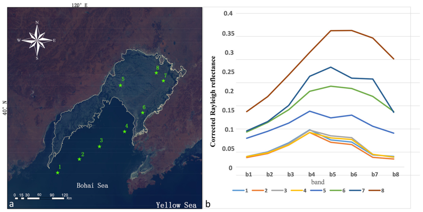
2. Study Area
3. Data
3.1. GOCI Images
3.2. SIT Observation
4. Method
4.1. Data Processing to Eliminate Atmospheric Effects
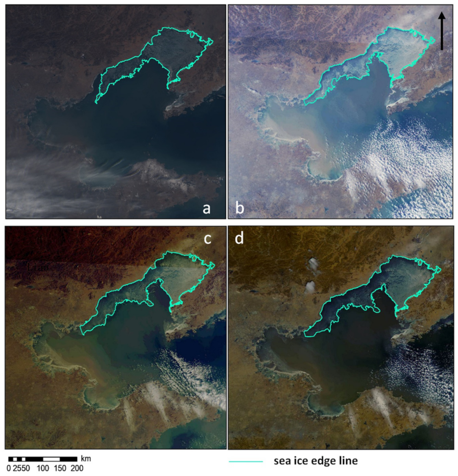
4.2. Sea Ice Extent Extraction
4.3. Optimization of the Ice Thickness Inversion Algorithm
4.3.1. Retrieval of SIT Using Several Bands
4.3.2. Retrieval of SIT Using All Bands
5. Temporal and Spatial Variation of the SIT in LDB
6. Discussion
6.1. Advantages and Limitations of the Retrieval Methods
6.2. The Effect of Snow on Sea Ice in the Retrieval Algorithm
7. Conclusions
Author Contributions
Funding
Data Availability Statement
Acknowledgments
Conflicts of Interest
References
- Curry, J.A.; Schramm, J.L.; Ebert, E.E. Sea ice-albedo climate feedback mechanism. J. Clim. 1995, 8, 240–247. [Google Scholar] [CrossRef]
- Eicken, H.; Lemke, P. The response of polar sea ice to climate variability and change. In Climate of the 21st Century, Changes and Risks; Lozán, J.L., Ed.; GEO: Hamburg, Germany, 2001; pp. 206–211. [Google Scholar]
- Serreze, M.C.; Stroeve, J. Arctic sea ice trends, variability and implications for seasonal ice forecasting. Philos. Trans. R. Soc. A Math. Phys. Eng. Sci. 2015, 373, 20140159. [Google Scholar] [CrossRef] [PubMed]
- Kapsch, M.; Graversen, R.G.; Tjernström, M.; Bintanja, R. The effect of downwelling longwave and shortwave radiation on Arctic summer sea ice. J. Clim. 2016, 29, 1143–1159. [Google Scholar] [CrossRef]
- Shi, W.; Wang, M. Sea ice properties in the Bohai Sea measured by MODIS-Aqua: 1. Satellite algorithm development. J. Mar. Syst. 2012, 95, 32–40. [Google Scholar] [CrossRef]
- Lemke, P.; Ren, J.; Alley, R.B.; Allison, I.; Carrasco, J.; Flato, G.; Fujii, Y.; Kaser, G.; Mote, P.; Thomas, R.H. Observations: Changes in Snow, Ice and Frozen Ground, Climate Change 2007: The Physical Science Basis; Contribution of Working Group i to the Fourth Assessment Report of the Intergovernmental Panel on Climate Change; Cambridge University Press: Cambridge, UK, 2007; pp. 337–383. [Google Scholar]
- Su, H.; Wang, Y.; Xiao, J.; Li, L. Improving MODIS sea ice detectability using gray level co-occurrence matrix texture analysis method: A case study in the Bohai Sea. ISPRS J. Photogramm. Remote Sens. 2013, 85, 13–20. [Google Scholar] [CrossRef]
- Shi, W.; Wang, M. Sea ice properties in the Bohai Sea measured by MODIS-Aqua: 2. Study of sea ice seasonal and interannual variability. J. Mar. Syst. 2012, 95, 41–49. [Google Scholar] [CrossRef]
- Liu, W.; Sheng, H.; Zhang, X. Sea ice thickness estimation in the Bohai Sea using geostationary ocean color imager data. Acta Oceanol. Sin. 2016, 35, 105–112. [Google Scholar] [CrossRef]
- Su, H.; Wang, Y.; Yang, J. Monitoring the spatiotemporal evolution of sea ice in the Bohai Sea in the 2009–2010 winter combining MODIS and meteorological data. Estuaries Coasts 2012, 35, 281–291. [Google Scholar] [CrossRef]
- Maksym, T.; Stammerjohn, S.; Ackley, S.; Massom, R. Antarctic Sea Ice—A Polar Opposite? Oceanography 2012, 25, 140–151. [Google Scholar] [CrossRef]
- Sumata, H.; Lavergne, T.; Girard Ardhuin, F.; Kimura, N.; Tschudi, M.A.; Kauker, F.; Karcher, M.; Gerdes, R. An intercomparison of A rctic ice drift products to deduce uncertainty estimates. J. Geophys. Res. Ocean. 2014, 119, 4887–4921. [Google Scholar] [CrossRef]
- Zhang, N.; Wu, Y.; Zhang, Q. Forecasting the evolution of the sea ice in the Liaodong Bay using meteorological data. Cold Reg. Sci. Technol. 2016, 125, 21–30. [Google Scholar] [CrossRef]
- Barber, D.G.; Thomas, A. The influence of cloud cover on the radiation budget, physical properties, and microwave scattering coefficient (sigma°) of first-year and multiyear sea ice. IEEE Trans. Geosci. Remote Sens. 1998, 36, 38–50. [Google Scholar] [CrossRef]
- Markus, T.; Cavalieri, D.; Gasiewski, A.; Klein, M.; Maslanik, J.; Powell, D.; Stankov, B.; Stroeve, J.C.; Sturm, M. Microwave Signatures of Snow on Sea Ice: Observations. IEEE Trans. Geosci. Remote Sens. 2006, 44, 3081–3090. [Google Scholar] [CrossRef]
- Yackel, J.J.; Barber, D. Observations of Snow Water Equivalent Change on Landfast First-Year Sea Ice in Winter Using Synthetic Aperture Radar Data. IEEE Trans. Geosci. Remote Sens. 2007, 45, 1005–1015. [Google Scholar] [CrossRef]
- Kurtz, N.T.; Farrell, S.L.; Studinger, M.; Galin, N.; Harbeck, J.P.; Lindsay, R.; Onana, V.D.; Panzer, B.; Sonntag, J.G. Sea ice thickness, freeboard, and snow depth products from Operation IceBridge airborne data. Cryosphere 2013, 7, 1035–1056. [Google Scholar] [CrossRef]
- Sturm, M.; Holmgren, J.; Perovich, D.K. Winter snow cover on the sea ice of the Arctic Ocean at the Surface Heat Budget of the Arctic Ocean (SHEBA): Temporal evolution and spatial variability. J. Geophys. Res. Ocean. 2002, 107, 23. [Google Scholar] [CrossRef]
- Nandan, V.; Geldsetzer, T.; Islam, T.; Yackel, J.J.; Gill, J.P.; Fuller, M.C.; Gunn, G.; Duguay, C. Ku-, X-and C-band measured and modeled microwave backscatter from a highly saline snow cover on first-year sea ice. Remote Sens. Environ. 2016, 187, 62–75. [Google Scholar] [CrossRef]
- Laxon, S.W.; Giles, K.A.; Ridout, A.L.; Wingham, D.J.; Willatt, R.; Cullen, R.; Kwok, R.; Schweiger, A.; Zhang, J.; Haas, C. CryoSat-2 estimates of Arctic sea ice thickness and volume. Geophys. Res. Lett. 2013, 40, 732–737. [Google Scholar] [CrossRef]
- Kwok, R.; Cunningham, G.F. ICESat over Arctic sea ice: Estimation of snow depth and ice thickness. J. Geophys. Res. Ocean. 2008, 113, C8010. [Google Scholar] [CrossRef]
- Kaleschke, L.; Tian-Kunze, X.; Maaß, N.; Mäkynen, M.; Drusch, M. Sea ice thickness retrieval from SMOS brightness temperatures during the Arctic freeze-up period. Geophys. Res. Lett. 2012, 39, 5501. [Google Scholar] [CrossRef]
- Tian-Kunze, X.; Kaleschke, L.; Maaß, N.; Mäkynen, M.; Serra, N.; Drusch, M.; Krumpen, T. SMOS-derived thin sea ice thickness: Algorithm baseline, product specifications and initial verification. Cryosphere 2014, 8, 997–1018. [Google Scholar] [CrossRef]
- Martin, S.; Drucker, R.; Kwok, R.; Holt, B. Improvements in the estimates of ice thickness and production in the Chukchi Sea polynyas derived from AMSR-E. Geophys. Res. Lett. 2005, 32, L05505. [Google Scholar] [CrossRef]
- Nihashi, S.; Ohshima, K.I.; Tamura, T.; Fukamachi, Y.; Saitoh, S.I. Thickness and production of sea ice in the Okhotsk Sea coastal polynyas from AMSR-E. J. Geophys. Res. Ocean. 2009, 114, C10025. [Google Scholar] [CrossRef]
- Wang, Z.Y.; Zhang, X.; Wang, S.S. Monitoring the Freeboard of the Drift Ice in the Bohai Sea Using the Cross-InSAR Technique with High-resolution TSX /TDX Data. Bull. Surv. Mapp. 2018, 25, 58–61. [Google Scholar]
- Zhang, X.; Zhang, J.; Meng, J.M. Polarimetric scattering characteristics based sea ice types classification by polarimetric synthetic aperture radar: Taking sea ice in the Bohai Sea for example. Acta Oceanol. Sin. 2013, 35, 95–101. [Google Scholar]
- Pan, S. Application Study in Monitoring the Bohai Sea Ice by Satellite Data of EOS/MODI. Master’s Thesis, Lanzhou University, Lanzhou, China, 1 May 2008. [Google Scholar]
- Ouyang, L.; Hui, F.; Zhu, L.; Cheng, X.; Cheng, B.; Shokr, M.; Zhao, J.; Ding, M.; Zeng, T. The spatiotemporal patterns of sea ice in the Bohai Sea during the winter seasons of 2000–2016. Int. J. Digit. Earth 2019, 12, 893–909. [Google Scholar] [CrossRef]
- Yan, Y.; Huang, K.; Shao, D.; Xu, Y.; Gu, W. Monitoring the characteristics of the Bohai Sea ice using high-resolution geostationary ocean color imager (GOCI) data. Sustainability 2019, 11, 777. [Google Scholar] [CrossRef]
- Ahn, J.H.; Park, Y.J.; Ryu, J.H.; Lee, B.; Oh, I.S. Development of atmospheric correction algorithm for Geostationary Ocean Color Imager (GOCI). Ocean Sci. J. 2012, 47, 247–259. [Google Scholar] [CrossRef]
- Wang, H. Study on Atmospheric Correction Methods for Water Color in Taihu Lake. Master’s Thesis, Nanjing Normal University, Nanjing, China, 1 April 2007. [Google Scholar]
- Perovich, D.K.; Grenfell, T.C. Laboratory Studies of the Optical Properties of Young Sea Ice. J. Glaciol. 1981, 27, 331–346. [Google Scholar] [CrossRef][Green Version]
- Zhang, Z.; Cao, Y.; Zhao, W. Wind characteristics and land-sea wind speed comparison in the Bohai Bay. Mar. Forecast. 2011, 28, 33–39. [Google Scholar]
- Ning, L.; Xie, F.; Gu, W.; Xu, Y.; Huang, S.; Yuan, S.; Cui, W.; Levy, J. Using remote sensing to estimate sea ice thickness in the Bohai Sea, China based on ice type. Int. J. Remote Sens. 2009, 30, 4539–4552. [Google Scholar] [CrossRef]
- Shi, W.; Yuan, S.; Xu, N.; Chen, W.; Liu, Y.; Liu, X. Analysis of floe velocity characteristics in small-scaled zone in offshore waters in the eastern coast of Liaodong Bay. Cold Reg. Sci. Technol. 2016, 126, 82–89. [Google Scholar] [CrossRef]
- Bai, X.; Wang, J.; Liu, Q.; Wang, D.; Liu, Y. Severe ice conditions in the Bohai Sea, China, and mild ice conditions in the great lakes during the 2009/10 winter: Links to El Nino and a strong negative arctic oscillation. J. Appl. Meteorol. Clim. 2011, 50, 1922–1935. [Google Scholar] [CrossRef]
- Bai, S.; Wu, H. Numerical sea ice forecast for the Bohai Sea. Acta Meteorol. Sin. 1998, 56, 139–153. [Google Scholar]
- Bai, S.; Liu, Q.; Li, H.; Wu, H. Sea ice in the Bohai Sea of China. Mar. Forecast. 1999, 16, 1–9. [Google Scholar]
- Cho, S.; Ahn, Y.; Ryu, J.; Kang, G.; Youn, H. Development of geostationary ocean color imager (GOCI). Korean J. Remote Sens. 2010, 26, 157–165. [Google Scholar]
- Ryu, J.; Han, H.; Cho, S.; Park, Y.; Ahn, Y. Overview of geostationary ocean color imager (GOCI) and GOCI data processing system (GDPS). Ocean Sci. J. 2012, 47, 223–233. [Google Scholar] [CrossRef]
- Zeng, T.; Shi, L.; Marko, M.; Cheng, B.; Zou, J.; Zhang, Z. Sea ice thickness analyses for the Bohai Sea using MODIS thermal infrared imagery. Acta Oceanol. Sin. 2016, 35, 96–104. [Google Scholar] [CrossRef]
- Zhao, M. Study of Cloud Removal Methods on Remote Sensing Images. Master’s Thesis, Tianjin University of Science and Technology, Tianjin, China, 1 November 2015. [Google Scholar]
- Liu, M.; Shen, F.; Ge, J.; Kong, Y.Z. Diurnal variation of suspended sediment concentration in Hangzhou Bay from geostationary satellite observation and its hydrodynamic analysis. J. Sediment Res. 2013, 1, 2. [Google Scholar]
- Hu, C. A novel ocean color index to detect floating algae in the global oceans. Remote Sens. Environ. 2009, 113, 2118–2129. [Google Scholar] [CrossRef]
- Chance, K.V.; Spurr, R.J. Ring effect studies: Rayleigh scattering, including molecular parameters for rotational Raman scattering, and the Fraunhofer spectrum. Appl. Opt. 1997, 36, 5224–5230. [Google Scholar] [CrossRef] [PubMed]
- Seasholtz, R.G.; Buggele, A.E.; Reeder, M.F. Flow measurements based on Rayleigh scattering and Fabry-Perot interferometer. Opt. Laser. Eng. 1997, 27, 543–570. [Google Scholar] [CrossRef]
- Haverkamp, D.; Soh, L.K.; Tsatsoulis, C. A comprehensive, automated approach to determining sea ice thickness from SAR data. IEEE Trans. Geosci. Remote Sens. 1995, 33, 46–57. [Google Scholar] [CrossRef]
- Su, H.; Wang, Y. Using MODIS data to estimate sea ice thickness in the Bohai Sea (China) in the 2009–2010 winter. J. Geophys. Res. Ocean. 2012, 117, C10018. [Google Scholar] [CrossRef]
- Shapiro, I.; Colony, R.; Vinje, T. April sea ice extent in the Barents Sea, 1850–2001. Polar Res. 2003, 22, 5–10. [Google Scholar]
- Grenfell, T.C. A radiative transfer model for sea ice with vertical structure variations. J. Geophys. Res. Ocean. 1991, 96, 16991–17001. [Google Scholar] [CrossRef]
- Xie, F.; Gu, W.; Yuan, Y.; Chen, Y. Estimation of sea ice resources in Liaodong gulf using remote sensing. Resour. Sci. 2003, 25, 17–23. [Google Scholar]
- Gardner, A.S.; Sharp, M.J. A review of snow and ice albedo and the development of a new physically based broadband albedo parameterization. J. Geophys. Res. Earth Surf. 2010, 115, F01009. [Google Scholar] [CrossRef]
- Grenfell, T.C.; Perovich, D.K. Spectral albedos of sea ice and incident solar irradiance in the southern Beaufort Sea. J. Geophys. Res. Ocean. 1984, 89, 3573. [Google Scholar] [CrossRef]
- Piwowar, J.M.; LeDrew, E.F. Principal components analysis of Arctic ice conditions between 1978 and 1987 as observed from the SMMR data record. Can. J. Remote Sens. 1996, 22, 390–403. [Google Scholar] [CrossRef]
- Liu, C.; Che, D.S.; Li, X.D. Sea ice distribution and influencing factors in the Yellow Sea and the Bohai Sea during winter. Resour. Sci. 2019, 41, 1167–1175. [Google Scholar]
- Cherukuru, N.; Martin, P.; Sanwlani, N.; Mujahid, A.; Müller, M. A Semi-Analytical Optical Remote Sensing Model to Estimate Suspended Sediment and Dissolved Organic Carbon in Tropical Coastal Waters Influenced by Peatland-Draining River Discharges off Sarawak, Borneo. Remote Sens. 2021, 13, 99. [Google Scholar] [CrossRef]
- Mishra, A.R.; Bajwa, S.G. Effect of suspended sediment and chlorophyll concentrations on water reflectance. Int. Agric. Eng. J. 2006, 15, 139–150. [Google Scholar]
- Wu, L.; Wu, H.; Sun, L.; Zhang, Y.; Liu, Y.; Wei, X. Retrieval of Sea Ice in the Bohai Sea from MODIS Data. Period. Ocean Univ. China 2006, 36, 173–179. [Google Scholar]
- Shi, L.; Zeng, T.; Mäkynen, M.; Cheng, B. Sea Ice Thickness Retrieval with MODIS Thermal Infrared Data over the Liaodong Bay during Winter 2012–2013. In Proceedings of the International Geoscience and Remote Sensing Symposium (IGARSS), Beijing, China, 10–15 July 2016; pp. 4857–4860. [Google Scholar]
- Kaufman, Y.J.; Tanré, D.; Boucher, O. A satellite view of aerosols in the climate system. Nature 2002, 419, 215–223. [Google Scholar] [CrossRef]
- Tian, L.; Wai, O.W.; Chen, X.; Li, W.; Li, J.; Li, W.; Zhang, H. Retrieval of total suspended matter concentration from Gaofen-1 Wide Field Imager (WFI) multispectral imagery with the assistance of Terra MODIS in turbid water–case in Deep Bay. Int. J. Remote Sens. 2016, 37, 3400–3413. [Google Scholar] [CrossRef]
- Lou, X.; Hu, C. Diurnal changes of a harmful algal bloom in the East China Sea: Observations from GOCI. Remote Sens. Environ. 2014, 140, 562–572. [Google Scholar] [CrossRef]
- Grenfell, T.C.; Warren, S.G.; Mullen, P.C. Reflection of solar radiation by the Antarctic snow surface at ultraviolet, visible, and nearinfrared wavelengths. J. Geophys. Res. Atmos. 1994, 99, 18669–18684. [Google Scholar] [CrossRef]
- Curry, J.A.; Schramm, J.L.; Rossow, W.B.; Randall, D. Overview of Arctic cloud and radiation characteristics. J. Clim. 1996, 9, 1731–1764. [Google Scholar] [CrossRef]
- Bergen, J.D. A possible relation of albedo to the density and grain size of natural snow cover. Water Resour. Res. 1975, 11, 745–746. [Google Scholar] [CrossRef]
- Bloch, M.R. Dust-induced albedo changes of polar ice sheets and glacierization. J. Glaciol. 1964, 5, 241–244. [Google Scholar] [CrossRef][Green Version]
- Green, R.O.; Dozier, J.; Roberts, D.; Painter, T. Spectral snow-reflectance models for grain-size and liquid-water fraction in melting snow for the solar-reflected spectrum. Ann. Glaciol. 2002, 34, 71–73. [Google Scholar] [CrossRef]


| Band | Central Wavelength (nm) | Bandwidth (nm) | SNR | Type | Primary Application | Time Period of Data Used |
|---|---|---|---|---|---|---|
| 1 | 412 | 20 | 1000 | Visible | Yellow substance and turbidity | 2012/02/04–2012/02/08 2013/01/03–2013/02/19 |
| 2 | 443 | 20 | 1090 | Visible | Chlorophyll absorption maximum | |
| 3 | 490 | 20 | 1170 | Visible | Chlorophyll and other pigments | |
| 4 | 555 | 20 | 1070 | Visible | Turbidity, suspended sediment | |
| 5 | 660 | 20 | 1010 | Visible | Atmospheric correction for turbid water, Baseline of fluorescence signal, Chlorophyll, suspended sediment | |
| 6 | 680 | 10 | 870 | Visible | Fluorescence signal | |
| 7 | 745 | 20 | 860 | NIR | Atmospheric correction and baseline of fluorescence signal | |
| 8 | 865 | 40 | 750 | NIR | Atmospheric correction, vegetation, water vapor reference over the ocean |
| JZ9-3 Oil Platform | JZ20-2 Oil Platform | ||||
|---|---|---|---|---|---|
| Index | Date | Mean | In Situ Data | Mean | In Situ Data |
| 1 | 4 February 2012 10:16 | 3.5 | 2–5 | 9 | 8–10 |
| 2 | 4 February 2012 13:16 | 3.5 | 2–5 | 7.5 | 5–10 |
| 3 | 4 February 2012 14:16 | 3.5 | 2–5 | 7.5 | 5–10 |
| 4 | 4 February 2012 15:16 | 3.5 | 2–5 | 6 | 4–8 |
| 5 | 6 February 2012 12:16 | 4 | 3–5 | 8 | 4–12 |
| 6 | 7 February 2012 8:16 | 6.5 | 4–9 | 11.5 | 8–15 |
| 7 | 7 February 2012 13:16 | 6.5 | 4–9 | 12 | 9–15 |
| 8 | 7 February 2012 15:16 | 6.5 | 4–9 | 12.5 | 10–15 |
| 9 | 8 February 2012 8:16 | 6.5 | 4–9 | 14 | 12–16 |
| 10 | 8 February 2012 9:16 | 5 | 4–6 | 18 | 14–22 |
| 11 | 8 February 2012 10:16 | 5.5 | 4–7 | 16 | 14–18 |
| 12 | 8 February 2012 11:16 | 5.5 | 4–7 | 16 | 14–18 |
| 13 | 8 February 2012 12:16 | 5 | 7–8 | 22.5 | 20–25 |
| 14 | 3 January 2013 10:16 | 5.5 | 4–7 | 11.5 | 8–15 |
| 15 | 7 January 2013 10:16 | 7 | 5–9 | 20 | 15–25 |
| 16 | 9 January 2013 10:16 | 7 | 5–9 | 22.5 | 15–30 |
| 17 | 18 January 2013 10:16 | 6.5 | 4–9 | 14 | 8–20 |
| 18 | 25 January 2013 10:16 | 5 | 3–7 | 5.5 | 3–8 |
| 19 | 4 February 2013 10:16 | 22.5 | 15–30 | 7.5 | 5–10 |
| 20 | 15 February 2013 10:16 | 13.5 | 12–15 | 11.5 | 8–15 |
| 21 | 19 February 2013 10:16 | 12.5 | 3–22 | 11.5 | 8–15 |
| 22 | 22 February 2013 10:16 | / | / | 11.5 | 8–15 |
| Component | PC1 | PC2 |
|---|---|---|
| Rrc1 | 0.292 | 0.851 |
| Rrc2 | 0.375 | 0.125 |
| Rrc3 | 0.373 | 0.126 |
| Rrc4 | 0.354 | −0.240 |
| Rrc5 | 0.351 | −0.096 |
| Rrc6 | 0.350 | −0.347 |
| Rrc7 | 0.369 | −0.235 |
| Rrc8 | 0.356 | −0.045 |
| Cumulative (%) | 78.230 | 85.487 |
| Station | Method | RMSE | Skill Score |
|---|---|---|---|
| JZ9-3 | 8 bands | 3.014 | 86.26 |
| PCA | 4.4933 | 67.65 | |
| 3 bands | 3.5829 | 80.96 | |
| Ouyang | 7.2248 | 44.32 | |
| JZ20-2 | 8 bands | 4.1805 | 78.24 |
| PCA | 4.5247 | 68.88 | |
| 3 bands | 4.2618 | 76.44 | |
| Ouyang | 6.9393 | 56.19 |
Publisher’s Note: MDPI stays neutral with regard to jurisdictional claims in published maps and institutional affiliations. |
© 2021 by the authors. Licensee MDPI, Basel, Switzerland. This article is an open access article distributed under the terms and conditions of the Creative Commons Attribution (CC BY) license (http://creativecommons.org/licenses/by/4.0/).
Share and Cite
Gu, F.; Zhang, R.; Tian-Kunze, X.; Han, B.; Zhu, L.; Cui, T.; Yang, Q. Sea Ice Thickness Retrieval Based on GOCI Remote Sensing Data: A Case Study. Remote Sens. 2021, 13, 936. https://doi.org/10.3390/rs13050936
Gu F, Zhang R, Tian-Kunze X, Han B, Zhu L, Cui T, Yang Q. Sea Ice Thickness Retrieval Based on GOCI Remote Sensing Data: A Case Study. Remote Sensing. 2021; 13(5):936. https://doi.org/10.3390/rs13050936
Chicago/Turabian StyleGu, Fengguan, Rui Zhang, Xiangshan Tian-Kunze, Bo Han, Lei Zhu, Tingwei Cui, and Qinghua Yang. 2021. "Sea Ice Thickness Retrieval Based on GOCI Remote Sensing Data: A Case Study" Remote Sensing 13, no. 5: 936. https://doi.org/10.3390/rs13050936
APA StyleGu, F., Zhang, R., Tian-Kunze, X., Han, B., Zhu, L., Cui, T., & Yang, Q. (2021). Sea Ice Thickness Retrieval Based on GOCI Remote Sensing Data: A Case Study. Remote Sensing, 13(5), 936. https://doi.org/10.3390/rs13050936