Abstract
New, accurate and generalizable methods are required to transform the ever-increasing amount of raw hyperspectral data into actionable knowledge for applications such as environmental monitoring and precision agriculture. Here, we apply advances in generative deep learning models to produce realistic synthetic hyperspectral vegetation data, whilst maintaining class relationships. Specifically, a Generative Adversarial Network (GAN) is trained using the Cramér distance on two vegetation hyperspectral datasets, demonstrating the ability to approximate the distribution of the training samples. Evaluation of the synthetic spectra shows that they respect many of the statistical properties of the real spectra, conforming well to the sampled distributions of all real classes. Creation of an augmented dataset consisting of synthetic and original samples was used to train multiple classifiers, with increases in classification accuracy seen under almost all circumstances. Both datasets showed improvements in classification accuracy ranging from a modest 0.16% for the Indian Pines set and a substantial increase of 7.0% for the New Zealand vegetation. Selection of synthetic samples from sparse or outlying regions of the feature space of real spectral classes demonstrated increased discriminatory power over those from more central portions of the distributions.
1. Introduction
Hyperspectral (HS) Earth observation has increased in popularity in recent years, driven by advancements in sensing technologies, increased data availability, research and institutional knowledge. The big data revolution of the 2000s and significant advances in data processing and machine learning (ML) have seen hyperspectral approaches used in a broad spectrum of applications, with methods of data acquisition covering wide-ranging spatial and temporal resolutions.
For researchers aiming to classify or evaluate vegetation, hyperspectral remote sensing offers rich spectral information detailing the influences of pigments, biochemistry, structure and water absorption whilst having the benefits of being non-destructive, rapid, and repeatable. These phenotypical variations imprint a sort of ‘spectral fingerprint’ that allows hyperspectral data to differentiate vegetation at taxonomic units ranging from broad ecological types to species and cultivars [1]. Acquiring labelled hyperspectral measurements of vegetation is expensive and time-consuming, resulting in limited training datasets for supervised classification techniques. However, this has been slightly alleviated through multi/hyperspectral data-sharing portals such as ECOSTRESS [2] and SPECCHIO [3]. Supervised classification of such high dimensional data has had to rely on feature reduction or selection techniques in order to overcome small training sample sizes and avoid the curse of dimensionality, also called the ‘Hughes phenomenon’. Additionally, the general requirement of large training datasets in ML has meant limited success has been had when trying to leverage recent ML progress towards classification of HS data, often leading to overfitting of models and poor generalizability.
Data augmentation (DA), the process of artificially increasing training sample size, has been implemented by the ML community when the problem of small or imbalanced datasets has been encountered. DA methods vary from simple pre-processing steps such as mirroring, rotating or scaling of images [4] to more complicated simulations [5,6] and generative models [7,8]. DA for timeseries or 1D data consists of the addition of noise, or methods such as time dilation, or cut and paste [9]. However, when dealing with non-spatial HS data, these methods would be unsuitable, as it is important to maintain reflectance and waveband relationships in order to ensure class labels are preserved. Methods of DA such as physics-based models [10], or noise injection [11,12] have been applied to HS data. Whilst successful, these methods are either simplifications of reality and require domain-dependent knowledge of target features in the case of physical models or rely upon random noise, potentially producing samples that only approximate the true distribution.
Generative adversarial networks (GANs) have been used successfully in many fields as a DA technique, often for images, timeseries/1D [13], sound synthesis [14], or anonymising medical data [15]. GANs consist of two neural networks trained in an adversarial manner. The generator (G) network produces synthetic copies mimicking the real training data while the discriminator (D) network attempts to identify whether a sample was from the real dataset or produced by G. The D is scored on its accuracy in identifying real from synthetic data, before passing feedback to G allowing it to learn how best to fool D and improve generation of synthetic samples [16].
The use of GANs to generate synthetic HS data is a relatively new field of study. GANs of varying architectures ranging from 1D spectral [17,18,19] to 2D [20], and 3D spectral-spatial [21] with differing data embeddings including individual spectra, HS images, and principal components have been examined. All have been able to demonstrate the ability to generate synthesized hyperspectral data and to improve classification outcomes to varying degrees whether through DA or conversion of the GANs discriminator model to a classifier. However, issues such as training instability and mode collapse, a common form of overfitting are prevalent.
The work presented in this paper applies advances in generative models to overcome limitations previously encountered by Audebert et al. [17] to produce more realistic synthetic HS vegetation data and eliminate reliance on PCA to reduce dimensionality and stabilise training. Specifically, we train a GAN using the Cramér distance on two vegetation HS datasets, demonstrating the ability to approximate the distribution of the training samples while encountering no evidence of mode collapse. We go on to demonstrate the use of these synthetic samples for data augmentation and reduced under-sampling of class distributions, as well as establishing a method to quantify the potential classification power of a synthetic sample by evaluating its relative position in feature space.
Generative Adversarial Networks—Background
GANs are a type of generative machine learning algorithm known as an implicit density model. This type of model does not directly estimate or fit the data distribution but rather generates its own data which is used to update the model. Since first being introduced by Goodfellow et al. [16] GANs have become a dominant field of study within ML/DL, with numerous variants and being described as “the most interesting idea in the last 10 years in machine learning” by a leading AI researcher [22]. Although sometimes utilizing non-neural network architectures, GANs generally consist of two neural networks, sometimes more, that compete against each other in a minimax game. This is where one neural network, the discriminator, attempts to reduce its “cost” or error as much as possible. This occurs in an adversarial manner, where the discriminator is trained to maximize the probability of correctly labelling whether a sample originates from the original data distribution or has been produced by the generator. Simultaneously, the generator is trained to minimize the probability that the discriminator correctly labels the sample [23].
As a result, the training of GANs is notoriously unstable, with issues such as the discriminator’s cost quickly becoming zero and providing no gradient to update the generator, or the generator converging onto a small subset of samples that regularly fool the discriminator, a common issue known as mode collapse. Considerable research has gone into attempting to alleviate these issues, improve training stability and improve quality of synthetic samples, so much so that during 2018 more than one GAN-related paper was being released every hour [23].
Unlike non-adversarial neural networks, the loss function of a GAN does not converge to an optimal state, making the loss values meaningless in respect to evaluating the performance of the model. In an attempt to alleviate this problem, the Wasserstein GAN (WGAN) was developed to use the Wasserstein distance, also known as the Earth Mover’s (EM) distance which results in an informative loss function for both D and G that converges to a minimum [24]. Rather than the D having sigmoid activation in its final layer producing a binary classification of real or fake, WGAN approximates the Wasserstein distance, which is a regression task detailing the distance between the real and fake distributions. Due to gradient loss being a common weakness with WGANs, they were improved by applying weight clipping to the losses with a gradient penalty (GP) [25], further improving training stability.
2. Experimental Design
Here, we implement the CramérGAN, a GAN variant using the Cramér/energy distance as the Ds loss, reportedly offering improved training stability and increased generative diversity over WGANs [26]. This choice was informed by our preliminary testing of wGAN and wGAN-GP that produced noisy synthesized samples and lower standard deviations, in addition to the learning instability and poor convergence previously reported for wGAN, which may explain mode collapse encountered by Audebert et al. [17].
Individual models were trained for each hyperspectral class, for a total of 38 models. Each model was trained for 50,000 epochs, at a ratio of 5:1 (5 training iterations of D for every 1 of G) using the Adam optimiser at a learning rate of 0.0001, with beta1 = 0.5 and beta2 = 0.9. The latent noise vector was generated from a normal distribution with length 100. The G consists of two fully connected dense layers followed by two convolution layers, all using the ReLu activation function save for the final convolution layer using Sigmoid activation. The final layer of G reshaped the output to be a 2D array with shape (batch size * number of bands). A similar architecture was used for the D, though reversed. Starting with two convolution layers into a flatten layer, followed by 2 fully connected dense layers, all layers of D used Leaky ReLu activation except the final layer which used a linear function (Figure 1) (Appendix A Table A1 and Table A2).
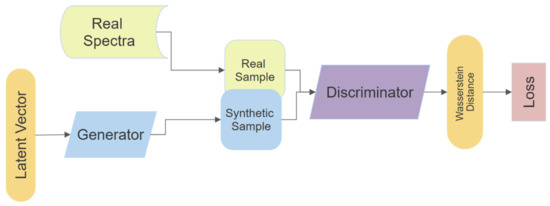
Figure 1.
Schematic of Generative Adversarial Network (GAN)architecture.
The three classification models (SVM, RF and NN) were evaluated in four permutations: trained on real data and evaluated on real data (real–real); trained on real data and evaluated on synthetic data (real–synthetic); trained on synthetic data and evaluated on synthetic data (synthetic–synthetic); and trained on synthetic data and evaluated on real data (synthetic–real). Each dataset was split into training and testing subsets with 10 times cross-validation. All synthetic datasets were restricted to the same number of samples per class as the real datasets unless specified otherwise. The real–real experiments were expected to have the highest accuracy and offer a baseline of comparison for the synthetic samples. If the accuracy of real–synthetic is significantly higher than real–real experiments, this potentially indicates that the generator has not fully learned the true distribution of the training samples. Conversely, accuracy being significantly lower could mean the synthetic samples are outside the true distribution and are an unrealistic representation of the spectra.
Extending this analysis, synthetic–synthetic and synthetic–real experiments were performed with the number of synthesized training samples increasing from 10 to 490 samples by increments of 10 samples per class. The real–synthetic and real–real experiments were included for comparison with a consistent number of training samples, though training and evaluation subsets differed every iteration. The initial DA experiment was performed with the same number of samples for real and synthetic datasets with the augmented set having twice the number before the number of synthetic samples were incremented by 10 from 10 to 490 samples per class.
The data augmentation capabilities of the synthetic spectra were evaluated by similar methods. First, the three classifiers were trained with either real, synthetic or both combined into an augmented dataset and tested against an evaluation dataset that was not used in the training of the GAN.
All code was written and executed in Python 3.7. The CramérGAN based upon [27] using the Tensorflow 1.8 framework. Support Vector Machine (SVM), and Random Forests (RF) classifiers make use of the Scikit-Learn 0.22.2 library, with Tensorflow 1.8 utilized for the neural network (NN) classifier. Additionally, Scikit-Learn 0.22.2 provided the dimensionality reduction functions for Principal Components Analysis (PCA) and t-distributed Stochastic Neighbourhood Embedding (t-SNE), with Uniform Manifold Approximation and Projection (UMAP) being a standalone library. Hyperparameters for all functions are provided in Appendix A.
2.1. Classification Power
Potential classification power of a sample was estimated with the C metric devised in Mountrakis and Xi [28] for the purpose of predicting the likelihood of correctly classifying an unknown sample by measuring its Euclidean distance in feature space to samples in the training dataset. Mountrakis and Xi [28] demonstrated a strong correlation between close proximity to number of training samples and likelihood of correctly being classified. The C metric is bound between −1 indicating low likelihood and 1 indicating high likelihood of successful classification.
Rather than focusing on the proximity of an unknown sample to a classifier’s training data, we are interested in the distance of each synthesized sample to that of the real data in order to evaluate any potential increase in information density. We hypothesise that a C value closer to the lower bound for a synthetic sample would indicate it being further away from real data points and of any synthetic samples with C values close to the upper bound. Such a sample could potentially contain greater discriminatory power for the classifier as it essentially fills a gap in feature space of the class distribution.
To determine whether some samples of the NZ dataset provide more information to the classifier than others, and that the improvement in classification accuracy is not purely from increased sample size, the distance of each generated sample was measured to all real samples of its class before being converted to a C value as per Mountrakis and Xi [28], with an h value range of 1–50 at increments of 1. Two data subsets were then created using the first 100 spectral samples after all synthetic samples were ordered by their C value in ascending (most distant) and descending (least distant) order. The first 100 samples from each ordered dataset rather than the full 500 were used to maximize differences, reduce computation time and simplify figures.
2.2. Datasets
Two hyperspectral datasets were used to train the GAN: Indian Pines agricultural land cover types (INDI); and New Zealand plant spectra (NZ). The Indian Pines dataset (INDI) recorded by the AVIRIS airborne hyperspectral imager over North-West Indiana, USA, is made available by Purdue University and comprises 145 × 145 pixels at 20 m spatial resolution and 224 spectral reflectance bands from 400 to 2500 nm [29]. Removal of water absorption bands by the provider reduced these to 200 wavebands, and then reflectance of each pixel was scaled between 0 and 1. Fifty pixels were randomly selected as training samples except for three classes with fewer than 50 total samples, for which 15 samples were used for training (Table 1).

Table 1.
Land cover classes, training and evaluation sample numbers for Indian Pines dataset.
The New Zealand (NZ) dataset used in this study is a subsample of hyperspectral spectra for 22 species taken from a dataset of 39 native New Zealand plant spectra collected from four different sites around the North Island of New Zealand and made available on the SPECCHIO database [3]. These spectra were acquired with an ASD FieldSpecPro spectroradiometer at 1 nm sampling intervals between 350 and 2500 nm. Following acquisition from the SPECCHIO database, spectra were resampled to 3 nm and noisy bands associated with atmospheric water absorption were removed (1326–1464, 1767–2004, 2337–2500) resulting in 540 bands per spectra. Eighty percent of samples per class were used for training the GAN and 20% held aside to evaluate classifier performance (Table 2).

Table 2.
Plant species classes, training and evaluation sample numbers for New Zealand dataset.
3. Results and Discussion
3.1. Mean and Standard Deviation of Training and Synthetic Spectra
In order to visualize similarities between synthetic and real spectra, the mean and standard deviation for each class are shown for the real, evaluation, and synthetic datasets. All low-frequency spectral features, as well as mean and standard deviations, appear to be reproduced with high accuracy by the GAN. At finer scales of 3–5 wavebands noise is present, most notably throughout the near infra-red (NIR) plateau (Figure 2). Smoothing of synthesized data by a number of methods resulted in either no improvement or decreased performance in a number of tests; for this reason, no pre-processing was performed on synthesized samples. Due to the high frequency and random nature of the noise, once mean and STD statistics are calculated the spectra appear smooth.

Figure 2.
Synthetic spectra of NZ class 0, 350–2400 nm at 3 nm bandwidths.
Class 0 is one of the NZ classes with the largest number of samples, resulting in its mean and standard deviation being similar between its real, evaluation, and synthetic subsets. However, this is not the case for all classes, with NZ-9 showing the mean and standard deviation of the randomly selected evaluation samples being vastly different to those of real and synthetic spectra (Figure 3). The same is seen amongst INDI classes, with class 2 matching across all 3 data subsets, and class 4 with only 40 samples showing substantial difference between evaluation and real samples, especially in the visible wavebands (Figure 4). Although some classes may struggle to represent the evaluation dataset due to the initial random splitting of the datasets, in general, mean and standard deviation of the synthetic samples very closely match the real training data.
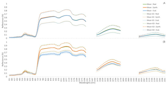
Figure 3.
Mean and +/− 1 STD for training (real), synthetic, and evaluation (real) datasets. (A) NZ class 0; Manuka (L. scoparium). (B) NZ class 9; Rata (M. robusta).
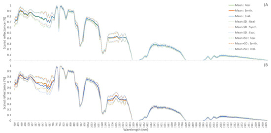
Figure 4.
Mean and +/− 1 STD for training (real), synthetic, and evaluation (real) datasets. (A) INDI class 2; corn-no-till. (B) INDI class 4; corn.
3.2. Generation and Distribution of Spectra
Here, we demonstrate the ability of the GAN to reproduce realistic spectral shapes and to capture the statistical distribution of the class populations. Three dimensionality reduction methods—PCA, t-SNE, and UMAP—were applied to both the real and synthetic datasets of INDI and NZ spectra to reduce their 200 and 540 wavebands (respectively) down to a plottable 2D space (Figure 5 and Figure 6). Upon visual inspection, the class clusters formed by the augmented data across all reduction methods mimic the distribution of those of the real data. Additionally, due to its small sample sizes the structure of clusters for the real NZ data is sparse and unclear, though is emphasised by the large number of synthetic samples.
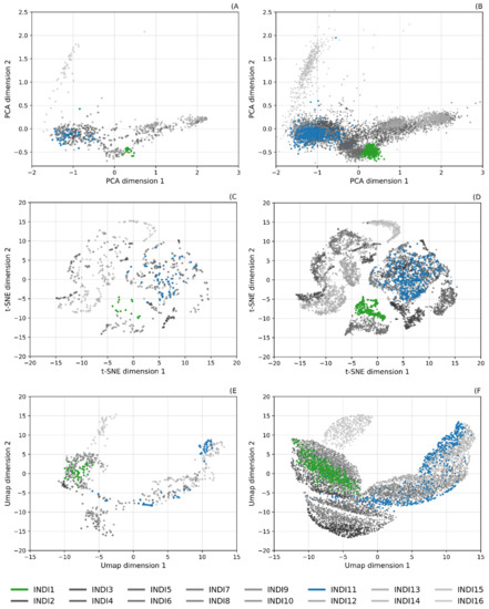
Figure 5.
Dimensional reduced representations of INDI real and synthetic datasets; highlighted classes: INDI1—Alfalfa (green); INDI11—Soybean-min-till (blue). (A) Real dataset; PCA reduction, (B) synthetic dataset; PCA reduction, (C) real dataset; t-SNE reduction, (D) synthetic dataset; t-SNE reduction, (E) real dataset; UMAP reduction, and (F) synthetic dataset; UMAP reduction.
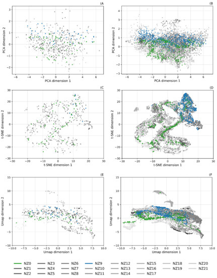
Figure 6.
Dimensional reduced representations of NZ real and synthetic datasets; + highlighted classes: NZ0—Manuka (L. scoparium) (green), NZ9—Rata (M. robusta) (blue). (A) Real dataset; PCA reduction, (B) synthetic dataset; PCA reduction, (C) real dataset; t-SNE reduction, (D) synthetic dataset; t-SNE reduction, (E) real dataset; UMAP reduction, and (F) synthetic dataset; UMAP reduction.
Such strong replication of the 2D representation of the classes is a good indication of the generative model’s ability to learn distributions. Even when the models are trained separately for each class, the relationship between classes is maintained. However, the increased sample number in the synthetic datasets do in some cases extend beyond the bounds of the real samples. Whilst some may represent potential outliers the majority are artefacts of increased sample sizes. This is most evident in the UMAP representation, where a parameter that defines minimum distance between samples can be set a larger value, which results in increased spread of samples in the 2D representation [30]. This is most notable in the INDI dataset, with classes 1, 7, and 8 extending more broadly than the real dataset (Figure 5F).
3.3. Training Classification Ability
In order to further examine the similarity of synthetic spectra to the real training data, three classifiers were trained (SVM, RF, NN), with four permutations of each (real–real, real–synthetic, synthetic–synthetic, and synthetic–real) (Table 3). With few exceptions, the neural network classifier outperformed the others, with SVM being the second most accurate, followed by RF. The INDI dataset recorded the highest accuracy for the real–real test with RF and NN classifiers at 74.76% and 84.13%, respectively, although the highest accuracy for the SVM classifier occurred during the synthetic–real test with 81.42% accuracy. Comparing the four combinations of real and synthetic, real–real had the highest accuracy for four experiments, with INDI synthetic–real with the SVM, and NZ real–synthetic with the RF classifier being the only exceptions.

Table 3.
Classification accuracies for classifiers trained on real or synthesized spectral data and evaluated on either real or synthesized data for both Indian Pines and New Zealand datasets based on real class sample sizes. Highest achieved accuracy for each classifier per dataset indicated in bold.
To further evaluate the synthetic spectra, synthetic–synthetic and synthetic–real experiments were performed with the number of synthesized training samples increasing from 10 to 490 samples by increments of 10 samples per class (Figure 7). Synthetic–synthetic accuracy improves with more samples: this too is to be expected as this simply adds more training samples from the same distribution. Most importantly, synthetic–real accuracy, though often slightly lagging behind synthetic–synthetic, improves in the same manner, indicating that the synthetic samples are a good representation of the true distribution and that increasing their number for training a classier is an effective method of data augmentation. The main exception to this is the NN NZ classier, where synthetic–synthetic quickly reaches ~100% accuracy, while synthetic–real maintains ~80% before slowly decreasing in accuracy as more samples are added. This could indicate the NN classifier focuses on different features than the other classifiers, potentially being more affected by the small-scale noise apparent in the NZ-generated samples as the noise is not as apparent in the INDI data and the INDI NN classifier does not show such a discrepancy between synthetic–synthetic and synthetic–real.
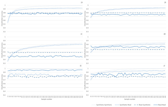
Figure 7.
Classification accuracies for classifiers trained on real or synthesized spectral data and evaluated on either real or synthesized data for both Indian Pines and New Zealand datasets ranging from 10 to 490 samples per class. (A) New Zealand dataset; SVM classifier, (B) Indian Pines dataset; SVM classifier, (C) New Zealand dataset; RF classifier, (D) Indian Pines dataset; RF classifier, (E) New Zealand dataset; NN classifier, and (F) Indian Pines dataset; NN classifier.
3.4. Data Augmentation
In order to test the viability of the synthetic data for data augmentation, the same three classifiers were trained with either real, synthetic or both combined into an augmented dataset and tested against an evaluation dataset (Table 4). All classifiers had higher accuracy when trained on the real dataset compared to synthetic, though the highest accuracy overall was with the augmented dataset. For the INDI data, this increase was minor, being < 1% for all classifiers. A far more significant improvement was seen for the NZ data with increases of 3.54% (to 86.55%), 0.53% (to 50.80%), and 3.73% (to 85.14%) for SVM, RF, and NN, respectively.

Table 4.
Classification accuracies for classifiers trained on real, synthesized, or augmented spectral data and evaluated on an evaluation dataset for both Indian Pines and New Zealand datasets based on real class sample sizes. Highest achieved accuracy for each classifier per dataset indicated in bold.
Of course, however, the number of synthetic samples does not have to be limited in such a manner. As with previous experiments the number of synthetic samples started at 10 and incremented by 10 to a total of 490, demonstrating the potential of this data augmentation method. Dramatic increases in accuracy were seen for the synthetic dataset, with the smallest increase being 5.13% for INDI-SVM occurring at 490 samples, the largest being 20.47% for NZ-RF at 420 samples. These increases brought the synthetic dataset very close to the accuracy of the real samples or even above in the cases of INDI-NN, NZ-RF, and NZ-NN. Increases in accuracy were also seen in the augmented dataset, though not as dramatic as those for the synthetic dataset. Improvements in accuracy ranged from 0.16% for INDI-SVM at 10 synthetic samples to 9.45% for NZ-RF at 280 synthetic samples. These improvements raise the highest accuracy for the INDI dataset from 70.40% to 70.56%, resulting in an increase of 0.16% over the highest achieved by just the real data. A larger increase was seen in the NZ dataset with the previous highest accuracy raising from 86.55% to 90.01%, an increase of 3.45% from the previous augmented classification with restricted sample size, and a 7% increase over the real dataset alone (Table 5).

Table 5.
Classification accuracies for classifiers trained on real, synthesized, or augmented spectral data and evaluated on an evaluation dataset for both Indian Pines and New Zealand datasets with sample sizes ranging from 10 to 490 per class for synthetic and augmented while real contained all real samples. Highest achieved accuracy for each classifier per dataset indicated in bold.
3.5. Classification Power of a Synthetic Sample
Ordering the synthetic samples by their C value before iteratively adding samples one at a time from each class to the training dataset of an SVM classifier shows the differing classification power of the synthetic samples from lower to upper bounds of C and vice versa (Figure 8).

Figure 8.
Classification accuracy of a SVM classifier for C metric ascending and descending ordered synthetic datasets incremented by single samples.
When in ascending order from lower to upper bounds, classification accuracy increases dramatically, reaching ~60% accuracy with ~100 samples, while 200 samples were required for similar accuracy in descending order. At approximately half the number of samples, accuracies converge, then increase at the same rate before reaching 80% accuracy at 500 samples. These classification accuracies (Figure 8) provide the first insight into increased discriminatory power associated with synthetic samples that occur at distance to real samples. Although not encountered here, a maximum limit to this distance would be present, with synthetic samples needing to remain within the bounds of their respective class distributions.
A similar, though reduced, trend can be seen when the ordered synthetic samples are used to augment the real dataset. Both ascending and descending datasets improve classification over that of the real dataset when samples are iteratively added to the classifiers training dataset (Figure 9). Despite descending ordered samples outperforming ascending at times, on average, ascending samples achieved ~1.5% higher accuracy across the classifications compared with the 79.72% to 78.24% accuracy of descending samples.

Figure 9.
Classification accuracy of a SVM classifier for C metric ascending and descending augmented datasets with randomly ordered real dataset incremented by single samples.
This artificial selection of synthetic data points distant or close to the real data influences sample distribution used to train the classifiers. As one might expect, the ordered data points come from the edges or sparse regions of the real data distribution, dramatically shifting the mean and standard deviation of the ordered datasets (Figure 10).

Figure 10.
(A) Mean and (B) STD of C metric ascending, descending, and randomly ordered synthetic datasets incremented by single samples.
The inclusion of synthetic data points selected at random provides a baseline for comparison with the ordered datasets. Once the number of samples increases beyond a few points, the means for descending and random converge and stay steady throughout. Mean values for ascending start significantly higher, though initially begin to converge towards the other datasets before plateauing at a higher level. Whilst being averaged across all classes and all wavebands of spectra, the mean reflectance for the ascending data is consistently higher. Standard deviation of the descending dataset is consistently low, only slightly increasing as samples are added. This is in stark contrast to the STD of the ascending dataset being ~5–6 x higher across all n samples. The mean of the randomly selected dataset occurs between the means of the two ordered, though closer to the ascending mean, indicating the samples that make up the descending dataset are highly conserved.
To further illustrate the relationship of the ordered datasets and the real distribution, a PCA of one of the classes is shown (Figure 11). As the mean and STD indicated, the descending samples are tightly grouped near the mean and densest area of the real data distribution, with the ascending samples generally occurring along the border of the real distribution. Whilst ascending selects for samples with low C and greater distance from real samples, it is important to note that these synthetic samples still appear to conform to the natural shape of the real distribution, a further indication the generative model is performing well.
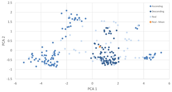
Figure 11.
PCA of NZ class 0; Manuka (L. scoparium) real samples, with first 100 samples of the ascending and descending C ordered synthetic datasets.
4. Conclusions
In this paper, we have successfully demonstrated the ability to train a generative machine learning model for synthesis of hyperspectral vegetation spectra. Evaluation of the synthetic spectra shows that they respect many of the statistical properties of the real spectra, conforming well to the sampled distributions of all real classes. Further to this, we have shown that the synthetic spectra generated by our models are suitable for data augmentation of a classification models training dataset. Addition of synthetic samples to the real training samples of a classifier produced increased overall classification accuracy under almost all circumstances examined. Of the two datasets, the New Zealand vegetation showed a maximum increase of 7.0% in classification accuracy, with Indian Pines demonstrating a more modest improvement of 0.16%. Selection of synthetic samples from sparse or outlying regions of the feature space of real spectral classes demonstrated increased discriminatory power over those from more central portions of the distributions. We believe further work regarding this could see targeted generation to maximize the information content of a synthetic sample that would result in improved classification accuracy and generalizability with a smaller augmented dataset. The use of these synthesized spectra to augment real spectral datasets allows for the training of classifiers that benefit from large sample numbers without a researcher needing to collect additional labelled spectra from the field. This is of increasing significance as modern machine and deep learning algorithms tend to require larger datasets.
Author Contributions
Conceptualization, A.H.; methodology, A.H.; data curation, A.H.; formal analysis, A.H.; writing—original draft preparation, A.H., K.C. and M.L.; writing—review and editing, A.H., K.C. and M.L.; supervision, K.C., M.L. All authors have read and agreed to the published version of the manuscript.
Funding
This research received no external funding.
Data Availability Statement
The publically available datasets used in our experiments are available at; Indian Pine Site 3 AVIRIS hyperspectral data image file, doi:10.4231/R7RX991C. New Zealand hyperspectral vegetation dataset, https://specchio.ch/.
Acknowledgments
Financial support for this research was provided by the Australian Government Research Training Program Scholarship and the University of Adelaide School of Biological Sciences.
Conflicts of Interest
The authors declare no conflict of interest.
Appendix A

Table A1.
Layer architecture of the GANs generator.
Table A1.
Layer architecture of the GANs generator.
| Layer Type/Parameters | Shape | Activation |
|---|---|---|
| Conv1D | (100,100) | ReLU |
| Conv1D | (100,50) | ReLU |
| Conv1D | (100,10) | ReLU |
| Flatten | ||
| Dense | 2048 | Leaky ReLU (alpha = 0.2) |
| Batch Normalization (momentum = 0.4) | ||
| Dropout (0.5) | ||
| Dense | 4096 | Leaky ReLU (alpha = 0.2) |
| Batch Normalization (momentum = 0.4) | ||
| Dropout (0.5) | ||
| Dense | 2048 | Leaky ReLU (alpha = 0.2) |
| Batch Normalization (momentum = 0.4) | ||
| Dropout (0.5) | ||
| Dense | 22 | Softmax |

Table A2.
Layer architecture of the GANs discriminator.
Table A2.
Layer architecture of the GANs discriminator.
| Layer Type/Parameters | Shape | Activation |
|---|---|---|
| Dense | 1024 | Leaky ReLU (alpha = 0.2) |
| Dense | 1024 | Leaky ReLU (alpha = 0.2) |
| Dense | 256 | Linear |

Table A3.
Epochs with Kullback–Leibler divergence loss, Adam optimiser with a learning rate of 0.00001, and a batch size of 32.
Table A3.
Epochs with Kullback–Leibler divergence loss, Adam optimiser with a learning rate of 0.00001, and a batch size of 32.
| Layer Type/Parameters | Shape | Activation |
|---|---|---|
| Conv1D | (100,100) | ReLU |
| Conv1D | (100,50) | ReLU |
| Conv1D | (100,10) | ReLU |
| Flatten | ||
| Dense | 2048 | Leaky ReLU (alpha = 0.2) |
| Batch Normalization (momentum = 0.4) | ||
| Dropout (0.5) | ||
| Dense | 4096 | Leaky ReLU (alpha = 0.2) |
| Batch Normalization (momentum = 0.4) | ||
| Dropout (0.5) | ||
| Dense | 2048 | Leaky ReLU (alpha = 0.2) |
| Batch Normalization (momentum = 0.4) | ||
| Dropout (0.5) | ||
| Dense | 22 | Softmax |

Table A4.
Hyperparameters used during UMAP dimension reduction for each dataset.
Table A4.
Hyperparameters used during UMAP dimension reduction for each dataset.
| Dataset | Number of Neighbours | Minimum Distance | Distance Metric |
|---|---|---|---|
| INDI | 20 | 1 | Canberra |
| NZ | 100 | 0.3 | Correlation |
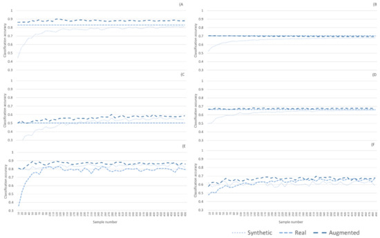
Figure A1.
(A) New Zealand dataset; SVM classifier, (B) Indian Pines dataset; SVM classifier, (C) New Zealand dataset; RF classifier, (D) Indian Pines dataset; RF classifier, (E) New Zealand dataset; NN classifier, and (F) Indian Pines dataset; NN classifier.
References
- Hennessy, A.; Clarke, K.; Lewis, M. Hyperspectral Classification of Plants: A Review of Waveband Selection Generalisability. Remote Sens. 2020, 12, 113. [Google Scholar] [CrossRef]
- JPL/NASA. ECOSTRESS. 2021. Available online: https://ecostress.jpl.nasa.gov/ (accessed on 28 May 2021).
- Hueni, A.; Chisholm, L.A.; Ong, C.C.H.; Malthus, T.J.; Wyatt, M.; Trim, S.A.; Schaepman, M.E.; Thankappan, M. The SPECCHIO Spectral Information System. IEEE J. Sel. Top. Appl. Earth Obs. Remote Sens. 2020, 13, 5789–5799. [Google Scholar] [CrossRef]
- Taylor, L.; Nitschke, G. Improving Deep Learning Using Generic Data Augmentation. 2017. Available online: https://arxiv.org/abs/1708.06020 (accessed on 12 November 2020).
- Wang, K. Synthetic DATA Generation and Adaptation for Object Detection in Smart Vending Machines. 2019. Available online: https://arxiv.org/abs/1904.12294 (accessed on 8 December 2020).
- Goodenough, A.A.; Brown, S.D. DIRSIG5: Next-Generation Remote Sensing Data and Image Simulation Framework. IEEE J. Sel. Top. Appl. Earth Obs. Remote Sens. 2017, 10, 4818–4833. [Google Scholar] [CrossRef]
- Bissoto, A.; Perez, F.V.M.; Valle, E.; Avila, S. Skin Lesion Synthesis with Generative Adversarial Networks. In Transactions on Petri Nets and Other Models of Concurrency XV; Springer Science and Business Media LLC: Cham, Switzerland, 2018; pp. 294–302. [Google Scholar]
- Wang, G.; Kang, W.; Wu, Q.; Wang, Z.; Gao, J. Generative Adversarial Network (GAN) Based Data Augmentation for Palmprint Recognition. In Proceedings of the 2018 Digital Image Computing: Techniques and Applications (DICTA), Canberra, Australia, 10–13 December 2018. [Google Scholar] [CrossRef]
- Wen, Q.; Sun, L.; Yang, F.; Song, X.; Gao, J.; Wang, X.; Xu, H. Time Series Data Augmentation for Deep Learning: A Survey. 2020. Available online: https://arxiv.org/abs/2002.12478 (accessed on 9 November 2020).
- Jacquemoud, S.; Verhoef, W.; Baret, F.; Bacour, C.; Zarco-Tejada, P.J.; Asner, G.P.; François, C.; Ustin, S.L. PROSPECT+SAIL models: A review of use for vegetation characterization. Remote Sens. Environ. 2009, 113, S56–S66. [Google Scholar] [CrossRef]
- Slavkovikj, V.; Verstockt, S.; De Neve, W.; Van Hoecke, S.; Van de Walle, R. Hyperspectral Image Classification with Convolutional Neural Networks. In Proceedings of the 23rd ACM international conference on Multimedia, Brisbane, Australia, 26–30 October 2015; pp. 1159–1162. [Google Scholar]
- Nalepa, J.; Myller, M.; Kawulok, M.; Smolka, B. On data augmentation for segmenting hyperspectral images. In Real-Time Image Processing and Deep Learning 2019; International Society for Optics and Photonics: Bellingham, WA, USA, 2019; Volume 10996, p. 1099609. [Google Scholar] [CrossRef]
- Harada, S.; Hayashi, H.; Uchida, S. Biosignal Generation and Latent Variable Analysis with Recurrent Generative Adversarial Networks. IEEE Access 2019, 7, 144292–144302. [Google Scholar] [CrossRef]
- Donahue, C.; McAuley, J.; Puckette, M. Adversarial Audio Synthesis. 2017. Available online: https://arxiv.org/abs/1802.04208 (accessed on 1 February 2020).
- Esteban, C.; Hyland, S.L.; Rätsch, G. Real-Valued (Medical) Time Series Generation with Recurrent Conditional Gans. Available online: https://arxiv.org/abs/1706.02633 (accessed on 12 August 2019).
- Goodfellow, I.J.; Pouget-Abadie, J.; Mirza, M.; Xu, B.; Warde-Farley, D.; Ozair, S.; Courville, A.; Bengio, Y. Generative adversarial nets. In Proceedings of the 27th International Conference on Neural Information Processing Systems—Volume 2 (NIPS’14), Cambridge, MA, USA, 8–13 December 2014; pp. 2672–2680. [Google Scholar]
- Audebert, N.; Le Saux, B.; Lefevre, S. Generative Adversarial Networks for Realistic Synthesis of Hyperspectral Samples. In Proceedings of the IGARSS 2018—2018 IEEE International Geoscience and Remote Sensing Symposium, Valencia, Spain, 22–27 July 2018; pp. 4359–4362. [Google Scholar]
- Zhan, Y.; Hu, D.; Wang, Y.; Yu, X. Semisupervised Hyperspectral Image Classification Based on Generative Adversarial Networks. IEEE Geosci. Remote Sens. Lett. 2017, 15, 212–216. [Google Scholar] [CrossRef]
- Xu, Y.; Du, B.; Zhang, L. Can We Generate Good Samples for Hyperspectral Classification?—A Generative Adversarial Network Based Method. In Proceedings of the IGARSS 2018—2018 IEEE International Geoscience and Remote Sensing Symposium, Valencia, Spain, 22–27 July 2018; pp. 5752–5755. [Google Scholar]
- Feng, J.; Yu, H.; Wang, L.; Cao, X.; Zhang, X.; Jiao, L. Classification of Hyperspectral Images Based on Multiclass Spatial–Spectral Generative Adversarial Networks. IEEE Trans. Geosci. Remote Sens. 2019, 57, 5329–5343. [Google Scholar] [CrossRef]
- Zhu, L.; Chen, Y.; Ghamisi, P.; Benediktsson, J.A. Generative Adversarial Networks for Hyperspectral Image Classification. IEEE Trans. Geosci. Remote Sens. 2018, 56, 5046–5063. [Google Scholar] [CrossRef]
- LeCun, Y. What Are Some Recent and Potentially Upcoming Breakthroughs in Deep Learning. 2016. Available online: https://www.quora.com/What-are-some-recent-and-potentially-upcoming-breakthroughs-in-deep-learning (accessed on 15 January 2021).
- Gui, J.; Sun, Z.; Wen, Y.; Tao, D.; Ye, J. A Review on Generative Adversarial Networks: Algorithms, Theory, and Applications. 2020. Available online: https://arxiv.org/abs/2001.06937 (accessed on 20 January 2021).
- Arjovsky, M.; Chintala, S.; Bottou, L. Wasserstein GAN. 2017. Available online: https://arxiv.org/abs/1701.07875 (accessed on 8 December 2019).
- Gulrajani, I.; Ahmed, F.; Arjovsky, M.; Dumoulin, V.; Courville, A. Improved training of wasserstein gans. arXiv 2017, arXiv:1704.00028. [Google Scholar]
- Bellemare, M.; Danihelka, I.; Dabney, W.; Mohamed, S.; Lakshminarayanan, B.; Hoyer, S.; Munos, R. The Cramer Distance as a Solution to Biased Wasserstein Gradients. 2017. Available online: https://arxiv.org/abs/1705.10743 (accessed on 12 March 2020).
- Song, J. Cramer-Gan. 2017. Available online: https://github.com/jiamings/cramer-gan (accessed on 28 December 2019).
- Mountrakis, G.; Xi, B. Assessing reference dataset representativeness through confidence metrics based on information density. ISPRS J. Photogramm. Remote Sens. 2013, 78, 129–147. [Google Scholar] [CrossRef]
- Baumgardner, M.F.; Biehl, L.L.; Landgrebe, D.A. 220 Band AVIRIS Hyperspectral Image Data Set: June 12, 1992 Indian Pine Test Site 3. 2015. Available online: https://purr.purdue.edu/publications/1947/1 (accessed on 6 July 2018).
- McInnes, L.; Healy, J.; Melville, J. UMAP: Uniform Manifold Approximation and Projection for Dimension Reduction. 2018. Available online: https://arxiv.org/abs/1802.03426 (accessed on 19 July 2019).
Publisher’s Note: MDPI stays neutral with regard to jurisdictional claims in published maps and institutional affiliations. |
© 2021 by the authors. Licensee MDPI, Basel, Switzerland. This article is an open access article distributed under the terms and conditions of the Creative Commons Attribution (CC BY) license (https://creativecommons.org/licenses/by/4.0/).