Article

Hyperspectral Image Super-Resolution with Self-Supervised Spectral-Spatial Residual Network

1
Key Laboratory of Spectral Imaging Technology CAS, Xi’an Institute of Optics and Precision Mechanics, Chinese Academy of Sciences, Xi’an 710119, China
2
University of Chinese Academy of Sciences, Beijing 100049, China
*
Author to whom correspondence should be addressed.
Remote Sens. 2021, 13(7), 1260; https://doi.org/10.3390/rs13071260
Submission received: 16 February 2021 / Revised: 23 March 2021 / Accepted: 23 March 2021 / Published: 26 March 2021
(This article belongs to the Special Issue Advances in Hyperspectral Data Exploitation)

Abstract

:
Recently, many convolutional networks have been built to fuse a low spatial resolution (LR) hyperspectral image (HSI) and a high spatial resolution (HR) multispectral image (MSI) to obtain HR HSIs. However, most deep learning-based methods are supervised methods, which require sufficient HR HSIs for supervised training. Collecting plenty of HR HSIs is laborious and time-consuming. In this paper, a self-supervised spectral-spatial residual network (SSRN) is proposed to alleviate dependence on a mass of HR HSIs. In SSRN, the fusion of HR MSIs and LR HSIs is considered a pixel-wise spectral mapping problem. Firstly, this paper assumes that the spectral mapping between HR MSIs and HR HSIs can be approximated by the spectral mapping between LR MSIs (derived from HR MSIs) and LR HSIs. Secondly, the spectral mapping between LR MSIs and LR HSIs is explored by SSRN. Finally, a self-supervised fine-tuning strategy is proposed to transfer the learned spectral mapping to generate HR HSIs. SSRN does not require HR HSIs as the supervised information in training. Simulated and real hyperspectral databases are utilized to verify the performance of SSRN.

1. Introduction

Hyperspectral imaging sensors collect hyperspectral images (HSIs) across many narrow spectral wavelengths, which contain rich physical properties of observed scenes [1]. HSIs with high spectral resolution are beneficial for various tasks, e.g., classification [2] and detection [3]. However, as the amount of incident energy is limited, observed HSIs usually have low spatial resolution (LR) [4]. Contrary to HSIs, observed multispectral images (MSIs) have high spatial resolution (HR) but low spectral resolution [5,6]. Exploring both MSIs and HSIs captured in the same scene is a feasible and effective way for improving the spatial resolution of HSIs [7].
Over decades, many methods [8,9] have been proposed to reconstruct the desired HR HSI by fusing HR MSIs and LR HSIs, including sparse representation-based methods [10,11], Bayesian-based methods [12,13], spectral unmixing-based methods [1,14], and tensor factorization-based methods [15,16]. Sparse representation-based, Bayesian-based, and spectral unmixing-based methods usually first learn spectral bases (or endmembers) from the LR HSI [9,10]. Then, the learned spectral bases are transformed to extract the sparse codes (or abundances) from the HR MSI. Finally, the desired HR HSI is reconstructed using the learned spectral bases and sparse codes. These methods usually treat the HR MSI and LR HSI as 2-D matrices, which result in the spatial structure information of HR MSIs and LR HSIs not being effectively exploited [15]. Tensor factorization-based methods [15,16] consider HR MSIs and LR HSIs as 3-D tensors to fully explore the spatial structure information of HR MSIs and LR HSIs. In general, previous methods mainly focus on exploiting various handcrafted priors (e.g., sparsity and low-rankness) to improve the quality of the reconstructed HR HSI [9]. However, sparsity and low-rankness priors may not hold in real complicated scenarios [17], which can result in unsatisfactory super-resolved results [18].
Recent works [19,20,21,22] usually build various deep learning (DL) architectures to learn deep priors for fusing HR MSIs and LR HSIs. Due to powerful feature learning capabilities, DL-based methods have shown superior performance. In most DL-based methods, deep networks are usually utilized to learn the deep priors between LR HSIs and HR HSIs [22,23,24]. For example, Li et al. [25] employed a Laplacian pyramid network instead of the bicubic interpolation to upsample HSIs for the guided filtering-based MSI and HSI fusion. Dian et al. [21] proposed to utilize a residual network to learn deep priors of HR HSIs. However, these methods are supervised methods, which require plentiful HR HSIs as the supervised information to optimize weight parameters of deep networks. It is an intractable problem to collect a mass of HR HSIs for supervised training [26].
To mitigate the dependence on HR HSIs as the supervised information, several works [26,27] have designed unsupervised deep networks. Yuan et al. [26] transferred the deep priors between LR and HR nature images to HSIs. Sidorov et al. [27] utilized a fully convolutional encoder–decoder network to explore deep hyperspectral priors. However, these methods [26,27] cannot exploit HR MSIs for reconstructing HR HSIs. To leverage both LR HSIs and the corresponding HR MSI, several works [17,28] attempted to build two-branch deep networks. Qu et al. [28] designed two sparse Dirichlet autoencoder networks: one for extracting spectral bases from LR HSI and the other for extracting spatial representations from HR MSIs. Ma et al. [17] proposed a generative adversarial network with two discriminators to reconstruct HR HSIs. One discriminator is utilized to preserve the spectral information of HR HSIs consistent with that of LR HSIs, and the other discriminator is designed to preserve the spatial structures of HR HSIs consistent with that of HR MSIs. However, these methods [17,28] ignore the potential spectral mapping relationship between the observed MSI and HSI.
In this paper, the fusion problem of HR MSIs and LR HSIs is considered a problem of learning the pixel-wise spectral mapping from MSIs to HSIs. The pixel-wise spectral mapping can be utilized to reconstruct hyperspectral pixels directly from multispectral pixels. Since the LR HSI and the reconstructed HR HSI contain the same observed scene, the spectral mapping between the HR MSI and HR HSI is assumed to be approximately equal to that between the corresponding LR MSI and LR HSI. In this paper, as shown in Figure 1, a self-supervised spectral-spatial residual network (SSRN) is proposed to learn the pixel-wise spectral mapping between LR MSIs and LR HSIs. Then, the learned spectral mapping is transferred to reconstruct the desired HR HSI from HR MSIs. In the proposed SSRN, the LR MSI utilized for training is the spatial degradation of HR MSIs. Additionally, SSRN takes the observed LR HSI instead of the HR HSI as supervised information in training. There are two advantages to consider the fusion problem of HR MSIs and LR HSIs as the problem of learning the pixel-wise spectral mapping. The first advantage is that reconstructing HR HSIs directly from HR MSIs, which contains the desired HR spatial structure information, can mitigate the distortion of spatial structures in HR HSIs. The second advantage is that there are plentiful multispectral and hyperspectral pixel pairs naturally between MSIs and HSIs, which are sufficient for training deep networks without the need to introduce other supervised information.
The proposed SSRN includes two modules: the spectral module and the spatial module. First, the spectral module is proposed to extract spectral features from MSIs. In the spectral module, the concatenation operation is employed to explore the complementarity among multi-layer features. Second, the spatial module is added following the spectral module to capture spectral-spatial features for facilitating learning of the spectral mapping. Especially, an attention mechanism is employed in the spatial module to make SSRN extract spectral-spatial features from homogeneous adjacent pixels, since homogeneous adjacent pixels in HSIs usually share similar spectral signatures. Finally, a self-supervised fine-tuning strategy is employed to further improve the performance of SSRN. In fact, the spatial degradation from the HR image to the LR image usually interferes with the spectral signatures of the LR image, which makes the spectral mapping between LR MSIs and LR HSIs slightly different from the spectral mapping between HR MSIs and HR HSIs. The self-supervised fine-tuning strategy is utilized to obtain the spectral mapping between HR MSIs and HR HSIs from the spectral mapping between LR MSIs and LR HSIs. The experimental results demonstrate that SSRN performs better than the state-of-the-art methods.
The major contributions of this paper are as follows:
  • A spectral-spatial residual network is proposed to consider the fusion of HR MSIs and LR HSIs as a pixel-wise spectral mapping problem. In SSRN, the HR HSI is estimated from the HR MSI at the desired spatial resolution, which can effectively preserve spatial structures of HR HSIs.
  • A self-supervised fine-tuning strategy is proposed to promote SSRN learning optimal spectral mapping. The self-supervised fine-tuning does not require HR HSIs as the supervised information.
  • A spatial module configured with the attention mechanism is proposed to explore the complementarity of adjacent pixels. The attention mechanism can explore the spectral-spatial features from homogeneous adjacent pixels, which is beneficial to the learning of pixel-wise spectral mapping.
The remaining sections are as follows. In Section 2, recent HSI super-resolution methods are reviewed. In Section 3, the proposed SSRN is introduced. The experimental results of SSRN and the compared methods are reported in Section 4. The performance of SSRN is discussed in Section 5. Finally, Section 6 concludes this paper.

2. Related Work

Many methods have been proposed to reconstruct HR HSIs by fusing the observed LR HSI and HR MSI. In light of whether deep networks are utilized, the existing methods are roughly categorized into traditional methods and DL-based methods.

2.1. Traditional Methods

According to different technique frameworks, traditional methods can be further divided into sparse representation-based methods, Bayesian-based methods, spectral unmixing-based methods, and tensor factorization-based methods.
Sparse representation-based methods [29] learn a dictionary from the observed LR HSI. The dictionary represents the reflectance spectrum of the scene and is then employed to learn the sparse code of HR MSIs. Akhtar et al. [30] proposed a generalization of the simultaneous orthogonal matching pursuit (GSOMP) method. Wei et al. [31] proposed a variational-based fusion method and designed a sparse regularization term.
Bayesian-based methods [32] intuitively interpret the process of fusion through the posterior distribution. Eismann et al. [33] proposed a maximum a posteriori probability (MAP) estimation method. Wei et al. [34] proposed a hierarchical Bayesian fusion method to fuse spectral images. Irmak et al. [35] proposed a MAP-based energy function to enhance the spatial resolution of HSI.
Spectral unmixing-based methods usually employ nonnegative matrix factorization to decompose HR MSIs and LR HSIs [36,37]. A classic method is coupled nonnegative matrix factorization (CNMF) [36]. In CNMF, HR MSIs and LR HSIs are alternately decomposed. Then, the estimated endmember matrix of the LR HSI and the estimated abundance matrix of the HR MSI are multiplied to reconstruct the HR HSI. Borsoi et al. [1] embedded an explicit parameter into a spectral unmixing-based method to model the spectral variability between the HR MSI and LR HSI.
Tensor factorization-based methods treat HSIs as a 3-D tensor to estimate a core tensor and the dictionaries of the width, height, and spectral modes [15,16]. Dian et al. [16] introduced the sparsity prior into tensor factorization to extract non-local spatial information from HR MSIs and spectral information from LR HSIs, respectively. Li et al. [38] proposed a coupled sparse tensor factorization to estimate the core tensor.
Traditional methods have achieved favorable performances by exploiting the priors (e.g., sparsity and low-rankness), but such priors may not hold in some complicated scenarios [9,17,18].

2.2. Deep Learning-Based Methods

Recently, many works have designed various deep networks for fusing HR MSIs and LR HSIs, which can be divided into supervised DL-based methods [39] and unsupervised DL-based methods [40].
Supervised DL-based methods usually exploit massive HR HSIs as training images to learn potential HSI priors or the mapping relationship between LR and HR HSIs [20,25]. Xie et al. [20] exploited the low-rankness prior of HSIs to construct an MSI and HSI fusion model, which can be optimized iteratively with the proximal gradient. Subsequently, the iterative optimization is unfolded into a convolutional network structure for end-to-end training. Wei et al. [23] proposed a residual convolutional network to learn the mapping relationship between LR MSIs and HR MSIs. To mitigate dependence on the point spread function and spectral response function, Wang et al. [24] proposed a blind iterative fusion network to iteratively optimize the observation model. Li et al. [39] proposed a two-stream network to reconstruct HR HSIs, where one is a 1-D convolutional stream to extract spectral features and the other is a 2-D convolutional stream to extract spatial features. However, in practice, collecting plenty of HR HSIs as supervised information for training is time-consuming and laborious [26,27].
Unsupervised DL-based methods are dedicated to leveraging spectral and spatial ingredients from the given HR MSI and LR HSI to reconstruct the desired HR HSI [17,28,41]. Huang et al. [42] utilized a sparse denoising autoencoder to learn the spatial mapping relationship between LR and HR panchromatic images, where LR panchromatic images are obtained from the spectral degradation of LR MSIs. Then, the learned spatial mapping relationship was exploited to improve the spatial resolution of each spectral band of LR MSIs. Fu et al. [40] proposed a plain network simply composed of five convolution layers to fuse HR MSIs and LR HSIs. The HR MSI was concatenated with the feature maps of every convolution layer to guide the spatial structure reconstruction of HR HSIs. Although recent methods have achieved superior performance [17,28], designing deep networks suitable for HSI super-resolution that do not require additional supervision information for training is still an open problem.

3. Materials and Methods

3.1. Proposed Method

3.1.1. Problem Formulation

The goal of the proposed SSRN is to estimate the HR HSI by fusing the observed HR MSI and LR HSI of the same scene. Let the HR HSI be X H R B × W × H , the observed LR HSI be X L R B × w × h , and the observed HR MSI be Y H R b × W × H , where B and b represent spectral band numbers, W and w represent the width, and H and h represent the height. The observed LR HSI has a higher spectral resolution and a lower spatial resolution than the observed HR MSI, i.e., W = D × w , H = D × h , and B b (D is the scaling factor). In fact, one pixel Y H ( i , j ) R b of Y H uniquely corresponds to one pixel X H ( i , j ) R B of X H , where ( i , j ) represents the spatial location in the ith row and the jth column. This paper exploits a convolutional network to learn a nonlinear pixel-wise spectral mapping F : R b R B that maps Y H ( i , j ) to X H ( i , j ) . The pixel-wise spectral mapping can be formulated as
X H = F ( Y H ) .
Since HR HSIs are difficult to obtain in practice [26,28], the proposed SSRN does not use HR HSIs as supervised information. In this paper, the spectral signatures of LR HSI X L are first used as the supervised information to learn the spectral mapping F ^ : R b R B between LR MSIs and LR HSIs. During the training phase, the input of SSRN is the LR MSI Y L R b × w × h and the output is the LR HSI X L . Y L is obtained by spatially blurring and then downsampling Y H .
Y L = E ( Y H ) ,
where E ( · ) represents the spatially blurring and downsampling operations [12]. Then, the learned spectral mapping F ^ between the LR MSI Y L and LR HSI X L is transformed to the spectral mapping F with a self-supervised fine-tuning strategy, which can reconstruct the HR HSI X H from the HR MSI Y H .
Previous methods [10,28,30,36] usually focus on extracting spectral ingredients (spectral bases or endmembers) from the LR HSI X L and extracting spatial ingredients (sparse codes or abundances) from the HR MSI Y H . Then, the spectral ingredients of X L and the spatial ingredients of Y H are utilized to reconstruct the HR HSI X H . However, the observed scene in the HR MSI Y H usually contains complex spatial distributions of land-covers; hence, there are still many challenges in accurately extracting spatial ingredients from HR MSI Y H [8,9]. In previous methods, inaccurate spatial ingredients extracted from the HR MSI Y H can cause spatial distortion of the reconstructed HR HSI. Different from previous methods [10,28,30,36], the proposed SSRN avoids the process of spatial ingredient extraction from HR MSI Y H . The proposed SSRN considers the fusion problem of HR MSI and LR HSI as a problem of spectral mapping learning. Based on the learned spectral mapping F, HR HSI X H is directly reconstructed from HR MSI Y H . All the spatial ingredients of HR MSI Y H can be used to reconstruct the HR HSI X H . Therefore, compared with previous methods, the proposed SSRN can better preserve the spatial structures of the reconstructed HR HSI.
The proposed method is similar to recent spectral resolution enhancement methods [43,44] that focus on learning the spectral mapping between MSIs and HSIs. However, the methods for spectral resolution enhancement are usually supervised training methods [45,46], which learn the spectral mapping from plentiful MSI and HSI pairs that are collected in other observed scenes. In contrast, in the HR MSI and LR HSI fusion task, the HR MSI and LR HSI are captured in the same observed scene. Our proposed method is a self-supervised training method specially designed for the HR MSI and LR HSI fusion task. The details of SSRN are introduced in the following subsections.

3.1.2. Architecture of SSRN

A detailed architecture of SSRN is shown in Figure 2. SSRN consists of two modules: the spectral module and the spatial module. In SSRN, the input is an MSI patch Y ^ R b × K × K and the output is an HSI patch X ^ R B × K × K , where b and B represent spectral band numbers and K × K represents the spatial size. First, a 1 × 1 convolution layer is used to generate initial shallow spectral features from the MSI patch Y ^ . Then, the spectral module is utilized to extract spectral features from the initial shallow spectral features, and the spatial module is added following the spectral module to extract spectral-spatial features to facilitate learning of spectral mapping.
In this paper, spectral features refer to the features of multispectral pixels in the spectral dimension, which do not involve any information of the spatially adjacent pixels. The spectral module mainly consists of several residual blocks and a multi-layer feature aggregation (MLFA) component. As shown in Figure 3, the setting of the residual blocks is similar to that in the literature [47], where the residual connection can facilitate the convergence of SSRN. In residual blocks, the kernel size of all convolution layers is set to 1 × 1 to ensure that spectral feature extraction is only performed in the spectral dimension of MSI. The different residual blocks can extract different spectral features, which are beneficial for learning spectral mapping [48,49]. To explore the complementarity among the features of different residual blocks, an MLFA component is employed to integrate these features into the final spectral feature. The MLFA component is composed of a concatenation layer and 1 × 1 convolution, which do not introduce any information from the spatially adjacent multispectral pixels.
The spatial module aims to extract complementary spatial information from adjacent pixels to learn spectral mapping. In this paper, the spatial information from adjacent pixels refers to the spatial structure information and spectrums contained in adjacent pixels. In practice, due to that adjacent pixels in real MSIs or HSIs potentially corresponding to the same object, adjacent pixels may have similar spectral signatures [50,51,52], which can be used as a prior to refine the reconstruct HR HSI. The adjacent pixels with similar spectral signatures are called homogeneous adjacent pixels. The spatial information of homogeneous adjacent pixels in HR MSI is beneficial in the learning of the pixel-wise spectral mapping between MSIs and HSIs [53]. Previous methods [43,44] usually use 3 × 3 convolution to extract spatial information. However, the 3 × 3 convolution can introduce the interference information from inhomogeneous adjacent pixels [2]. In this paper, the spatial module employs a self-attention module [54] to extract spectral-spatial features from the homogeneous adjacent pixels. The self-attention module can capture homogeneous adjacent pixels based on the correlation between different pixels [54] and then aggregate the information from these homogeneous adjacent pixels to generate spectral-spatial features. The details of the self-attention module are shown in Figure 3. The self-attention module takes the final spectral feature from the spectral module as the input and outputs the spectral-spatial features. The final spectral feature is denoted as S R C × K × K , where C is the channel number and K × K is the spatial size. First, S is fed into three 1 × 1 convolution layers to generate abstract features f ( S ) R C × K × K , g ( S ) R C × K × K , and n ( S ) R C × K × K , respectively. Second, f ( S ) , g ( S ) , and n ( S ) are reshaped to f ¯ ( S ) , g ¯ ( S ) , and n ¯ ( S ) R C × M , where M = K × K . Each column of the reshaped f ¯ ( S ) , g ¯ ( S ) , and n ¯ ( S ) represents the spectral feature of a certain pixel. The correlation among pixels in spectral features is calculated as follows
N = f ¯ ( S ) T g ¯ ( S ) ,
where ( · ) T denotes the transpose and N R M × M . A softmax function is employed to normalize the value of all elements in N to the range [ 0 , 1 ] . Then, the spectral-spatial features are generated by multiplying n ¯ ( S ) with the normalized correlation N . With the normalized correlation N , the homogeneous pixels from adjacent regions can be aggregated to facilitate the learning of the spectral mapping. Finally, the shape of spectral-spatial features is reshaped to R C × K × K for the following operations. After the self-attention module, a 1 × 1 convolution layer with B kernels is utilized to reconstruct the desired HR HSI from the spectral-spatial features.
In the proposed SSRN, the kernel size of all convolution layers is set to 1 × 1 , which can mitigate the difficulty of training SSRN caused by too many weight parameters.

3.1.3. Loss Function

In the proposed SSRN, a reconstruction loss L r e c and a cosine similarity loss L c o s are employed as the loss functions. Let U represent the generated HSI and V represent the ground truth. For convenience, U and V are reshaped to R P × Q , where P is the number of spectral bands and Q is the number of pixels. Each column of U and V represents the spectral vector of a hyperspectral pixel. The reconstruction loss L r e c is a classic metric function that measures the numerical differences between two HSIs. L r e c is defined as
L r e c ( U , V ) = U V F 2 ,
where · F represents the Frobenius norm. The cosine similarity loss L c o s measures the spectral distortion based on the angle between two spectral signatures. L c o s is defined as
L c o s ( U , V ) = 1 1 Q i = 1 Q U ( i ) · V ( i ) U ( i ) 2 V ( i ) 2 ,
where U ( i ) is the ith column of U that denotes the spectral vector of the ith pixel of U and V ( i ) is the ith column of V that denotes the spectral vector of the ith pixel of V ( 1 i Q ).
In the training phase, the LR MSI Y L and the LR HSI X L are cropped into small patches for training. Let Y ^ L R b × K × K be the LR MSI patch cropped from Y L , X ^ L R B × K × K be the corresponding LR HSI patch cropped from X L , and X ¯ L = F ^ ( Y ^ L ) R B × K × K be the reconstructed LR HSI patch. To facilitate calculation of the loss, Y ^ L is reshaped to R b × M , and X ^ L and X ¯ L are reshaped to R B × M , where M = K × K . The details of the loss function in SSRN are as follows.
First, the loss L o s s H S I between the reconstructed X ¯ L and the ground truth X ^ L are measured by the reconstruction loss L r e c and the cosine similarity loss L c o s .
L o s s H S I ( X ¯ L , X ^ L ) = L r e c ( X ¯ L , X ^ L ) + λ L c o s ( X ¯ L , X ^ L ) ,
where λ is the balancing parameter to control the tradeoff between L r e c and L c o s .
Second, according to the observation model, the LR MSI patch Y ^ L is the spectral degradation of the LR HSI patch X ^ L [14], which can be formulated as
Y ^ L = R ( X ^ L ) ,
where R ( · ) represents the spectral degradation. This means that the spectral degradation of the reconstructed HSI patch X ¯ L should also be consistent with the input MSI patch Y ^ L . To maintain the consistency between R ( X ¯ L ) and Y ^ L , another loss function L o s s M S I is established in this paper. Similar to L o s s H S I , L o s s M S I is formulated as
L o s s M S I ( R ( X ¯ L ) , Y ^ L ) = L r e c ( R ( X ¯ L ) , Y ^ L ) + β L c o s ( R ( X ¯ L ) , Y ^ L ) ,
where β is simply set to the same value as λ of Equation (6), since the second terms in Equations (6) and (8) are all the cosine similarity loss. Overall, the loss function of SSRN is set as
L o s s t r a i n = L o s s H S I ( X ¯ L , X ^ L ) + ϕ L o s s M S I ( R ( X ¯ L ) , Y ^ L ) .
In the proposed SSRN, L o s s H S I and L o s s M S I are equally important for reconstructing HR HSI. Therefore, ϕ is simply set to 1 in the following experiments.

3.1.4. Self-Supervised Fine-Tuning

This paper assumes that the pixel-wise spectral mapping F between HR MSI and HR HSI can be estimated on the basis of the pixel-wise spectral mapping F ^ between LR MSI and LR HSI. The training process of the proposed SSRN includes two stages: the pretraining stage and the fine-tuning stage. In the pretraining stage, the pixel-wise spectral mapping F ^ can be easily learned from the paired LR MSI patches and LR HSI patches using the proposed SSRN. In this stage, the proposed SSRN is supervised by LR MSIs and LR HSIs simultaneously. In fact, the spectral signatures of LR MSIs and LR HSIs are usually influenced by spatial degradation. The spectral mapping F ^ is not exactly equal to the spectral mapping F. Hence, in this paper, a fine-tuning strategy is proposed to further estimate the spectral mapping F from the spectral mapping F ^ . The SSRN trained with LR MSIs and LR HSIs serves as a pretrained network. Then, in the fine-tuning stage, the pretrained SSRN is further fine-tuned with the HR MSI. Since the HR HSI is hard to be obtained in practice, SSRN does not utilize the HR HSI as supervised information in training. Therefore, Equation (6) cannot be employed as the loss function in the fine-tuning stage. Equation (8) is employed as the fine-tuning loss L o s s F T to maintain the consistency between R ( X ¯ H ) and Y ^ H , where R ( · ) has the same definition as that in Equation (7), X ¯ H is the reconstructed HR HSI patch, and Y ^ H is the input HR MSI patch. L o s s F T can be expressed as
L o s s F T = L o s s M S I ( R ( X ¯ H ) , Y ^ H ) .
In the fine-tuning stage, the proposed SSRN is only supervised by HR MSI. Therefore, the fine-tuning stage is a self-supervised training style. After fine-tuning, the spectral mapping F between HR MSI and HR HSI is obtained. The desired HR HSI can be reconstructed with Equation (1).

3.2. Software and Package

The proposed SSRN is implemented in a computer workstation that is configured with the Ubuntu 14.04 system, 64G RAM, Intel Core i7-5930K, and NVIDIA TITAN X. The software used in the experiments is PyCharm. The packages used in the experiments include Python, TensorFlow, NumPy, and SciPy.

3.3. Databases

To evaluate the performance of SSRN, the experiments are conducted on simulated databases and real databases, respectively. First, the Pavia University (PU) database (http://www.ehu.eus/ccwintco/index.php?title=Hyperspectral_Remote_Sensing_Scenes#Pavia_University_scene, accessed on 16 December 2020) and the Washington DC Mall (WDCM) database (https://engineering.purdue.edu/~biehl/MultiSpec/hyperspectral.html, accessed on 16 December 2020) are utilized to simulate MSIs for experiments. Then, the Paris database (https://github.com/alfaiate/HySure/tree/master/data, accessed on 17 December 2020) [12] and the Ivanpah Playa database (https://github.com/ricardoborsoi/FuVarRelease/tree/master/DATA, accessed on 17 December 2020) [1], which contain both real MSIs and HSIs, are employed to conduct experiments. Finally, the CAVE database (https://www.cs.columbia.edu/CAVE/databases/multispectral/, accessed on 19 December 2020) [55] is employed to further explore the performance of SSRN.
The PU database is captured by the ROSIS sensor over Pavia University. The PU database contains an HSI with 103 spectral bands and 610 × 340 pixels. The WDCM database is collected by the HYDICE sensor over the National Mall. The WDCM database consists of an HSI with 191 spectral bands and 1280 × 307 pixels. Similar to the literature [37], a 200 × 200 subimage of the PU database and a 240 × 240 subimage of the WDCM database are utilized for experiments. The original HSIs in the PU and WDCM databases are regarded as the ground truth. The ground truth is blurred and then spatially downsampled with the scaling factor of 4 to simulate the observed LR HSI. The observed HR MSI is obtained by spectrally downsampling the ground truth. The setting of the spectral response function is the same as that in the literature [37].
The Paris database contains an HSI captured by the hyperion instrument and an MSI collected by the ALI instrument [12]. The HSI contains 128 spectral bands. The MSI contains 9 spectral bands. Both the HSI and the MSI have 72 × 72 pixels. The Ivanpah Playa database consists of an HSI with 173 spectral bands and an MSI with 10 spectral bands. The HSI and the MSI on the Ivanpah Playa database contain 80 × 128 pixels. According to the literature [1], the HSIs on the Paris and Ivanpah Playa databases are treated as the ground truth, which are blurred and spatially downsampled with the scaling factor of 4 to generate the observed LR HSI. The MSIs on the Paris and Ivanpah Playa databases are treated as the observed HR MSI.
The CAVE database contains 32 HSIs, which are captured by the cooled charge-coupled device (CCD) camera on the ground [55]. On the CAVE database, each HSI consists of 512 × 512 pixels, where each pixel is composed of 31 spectral bands ranging from 400 nm to 700 nm. Following the literature [56], the original HSIs on the CAVE database are treated as the ground truth. Then, the ground truth is blurred and spatially downsampled with the scaling factor of 4 to obtain the observed LR HSI. The ground truth is spectrally downsampled by the spectral response function of Nikon D700 (https://maxmax.com/spectral_response.htm, accessed on 19 December 2020) to obtain the observed HR MSI.

3.4. Evaluation Metrics

Five quantitative quality metrics are employed for performance evaluation, including peak signal-to-noise ratio (PSNR), spectral angle mapper (SAM), universal image quality index (UIQI), erreur relative globale adimensionnelle de synthèse (ERGAS), and root mean squared error (RMSE). PSNR measures the spatial reconstruction quality of each spectral band in the reconstructed HR HSI. SAM measures the spectral distortions of each hyperspectral pixel in the reconstructed HR HSI. UIQI measures the spatial structural similarity between the reconstructed HR HSI and the ground truth based on the combination of luminance, contrast, and correlation comparisons. ERGAS takes into account the ratio of ground sample distances between HR MSI and LR HSI to measure the global statistical quality of the reconstructed HR HSI. RMSE measures the global statistical error between the reconstructed HR HSI and the ground truth. The larger values of PSNR and UIQI indicate the better quality of the reconstructed HR HSI. When the values of SAM, ERGAS, and RMSE are smaller, the quality of the reconstructed HR HSI is better. The best value of PSNR is + . The best value of SAM is 0. The best value of UIQI is 1. The best values of ERGAS and RMSE are 0.
In this paper, the ground truth X ˜ H R B × W × H and the reconstructed HR HSI X H R B × W × H are converted into 8-bit images to calculate quantitative performance, where B, W, and H are the numbers of the band, width, and height, respectively. The formulations of the above quality metrics for the ground truth X ˜ H and the reconstructed HR HSI X H are given below.
PSNR is formulated as
PSNR = 1 B i = 1 B 10 log 10 m a x ( X ˜ H i ) 2 1 W × H j = 1 W × H X ˜ H i j X H i j 2 ,
where m a x ( X ˜ H i ) represents the maximum pixel value in the ith band of X ˜ H . X ˜ H i j and X H i j ( 1 i B , 1 j W × H ) represent the jth pixel in the ith band of X ˜ H and X H , respectively.
SAM is formulated as
SAM = 1 W × H j = 1 W × H arccos X ˜ H j T X H j X ˜ H j 2 X H j 2 ,
where X ˜ H j R B × 1 and X H j R B × 1 ( 1 j W × H ) denote the spectra of the jth pixel of X ˜ H and X H , respectively. ( · ) T denotes the transpose, and · 2 denotes the 2 vector norm.
UIQI is formulated as
UIQI = 1 B i = 1 B 1 Z q = 1 Z 4 μ z ˜ i q μ z i q σ z ˜ i q z i q μ z ˜ i q 2 + μ z i q 2 σ z ˜ i q 2 + σ z i q 2 ,
where a sliding window moving pixel by pixel is used to divide the ith band of X ˜ H and X H at the same position into Z image patch pairs z ˜ i q and z i q ( 1 i B , 1 q Z ), respectively. Z is the image patch pair number. μ z ˜ i q and μ z i q are mean pixel values of image patches z ˜ i q and z i q , respectively. σ z ˜ i q and σ z i q are the corresponding variance. σ z ˜ i q z i q is the covariance.
ERGAS is formulated as
ERGAS = 100 d 1 B i = 1 B 1 W × H j = 1 W × H X ˜ H i j X H i j 2 μ X ˜ H i 2 ,
where d is the ratio of ground sample distances between HR MSI and LR HSI. μ X ˜ H i ( 1 i B ) denotes the mean pixel value in the ith band of the ground truth HSI X ˜ H .
RMSE is formulated as
RMSE = 1 B i = 1 B 1 W × H j = 1 W × H X ˜ H i j X H i j 2 ,
where X ˜ H i j and X H i j ( 1 i B , 1 j W × H ) represent the jth pixel in the ith band of X ˜ H and X H , respectively.

4. Results

4.1. Parameter Settings of SSRN

This subsection explores the parameter settings of SSRN. The WDCM database has plenty of spectral bands and contains complicated land-cover distributions, making the fusion task challenging [16]. Therefore, the WDCM database is utilized for parameter setting experiments. For convenience, this subsection directly uses PSNR and SAM to measure the quality of the reconstructed HR HSI. Moreover, the fine-tuning strategy is not employed in the parameter setting experiments.

4.1.1. Number of Convolutional Kernels

In the experiments, the spatial size of input image patches is set as 4 × 4 . The number of training epochs is set as 200. The learning rate is initially set as 0.01, which then drops by a factor of 10 after 100 epochs. The balancing parameter λ in the loss function is initially set as 0.1. The number of residual blocks is set as 3. For convenience, all convolution layers of SSRN (except the last convolution layer) are configured with the same number of convolutional kernels, which is set as 16, 32, 64, 128, 256m and 512 for the experiments. The PSNR and SAM of SSRN with different numbers of convolutional kernels on the WDCM database are shown in Table 1. As the kernel number increases from 16 to 256, the performance of SSRN increases. As the kernel number increases from 256 to 512, the performance of SSRN decreases due to too many weight parameters, making SSRN training difficult. As shown in Table 1, the number of convolutional kernels in SSRN except the last convolution layer is set as 256 in the following experiments.

4.1.2. Number of Residual Blocks

SSRN utilizes several residual blocks to extract spectral features from the MSI. To explore the effects of different numbers of residual blocks on the performance of SSRN, the number of residual blocks is set as 1, 2, 3, 4, 5, and 6 for the experiments. The PSNR and SAM of SSRN on the WDCM database are shown in Table 2. SSRN with 4 residual blocks achieves the best performance, where the PSNR and SAM are 33.167 and 1.213, respectively. In following experiments, the residual block number of SSRN is set as 4.

4.1.3. Balancing Parameter λ

The balancing parameter λ is a key parameter that controls the tradeoff between the reconstruction loss and the cosine similarity loss in SSRN. If the value of the balancing parameter λ is too small, the cosine similarity loss in SSRN will be invalidated, resulting in a large SAM value of the reconstructed HR HSI. If the value of the balancing parameter λ is too large, the reconstruction loss will be invalidated, resulting in a decrease in the quality of the reconstructed HR HSI. To explore the impacts of the balancing parameter λ on the performance of SSRN, λ is set as 0.001, 0.01, 0.1, 1, 5, and 10 for the experiments. The PSNR and SAM of SSRN with different balancing parameter λ are shown in Table 3. As λ increases from 0.001 to 0.1, the performance of SSRN increases. However, as λ increases from 0.1 to 10, the performance of SSRN decreases. The balancing parameter λ of SSRN is set as 0.1 in the following experiments.

4.2. Ablation Study

The proposed SSRN can be specifically decomposed into five components, including the basic network, the MLFA component, the spatial module, the cosine similarity loss, and the fine-tuning. The basic network refers to the proposed spectral module without the MLFA, which can be utilized to coarsely learn the pixel-wise spectral mapping. The loss function of the basic network is a reconstruction loss. The other four components are utilized to improve the performance of this basic network. In this subsection, the ablation experiments for these four components are conducted on the WDCM database. The experimental results are shown in Table 4. The basic network achieves the worst performance. It is indicated that spatial features are not adequately exploited by the basic network. The MLFA component is added to the basic network to demonstrate that aggregating features of different convolution layers can improve the performance of the basic network. After further introducing the spatial module in the basic network and MLFA, the PSNR of the estimated HSI improved. Although the spatial module can improve the spatial quality of the estimated HSI, it cannot significantly reduce the spectral distortion. Then, the cosine similarity loss is further added into the basic network combined with the MLFA and the spatial module. As shown in Table 4, the cosine similarity loss can effectively alleviate the problem of spectral distortion in the estimated HSI. Finally, the fine-tuning strategy is added into the basic network combined with other three components. The proposed SSRN shows superior performance, which demonstrates the effectiveness of the fine-tuning strategy. Therefore, the MLFA, the spatial module, the cosine similarity loss, and the fine-tuning are all crucial components for the proposed SSRN.

4.3. Comparisons with Other Methods on Simulated Databases

In this subsection, the PU and WDCM databases are employed to simulate HR MSIs to evaluate the proposed SSRN. The proposed SSRN is compared with several state-of-the-art HSI super-resolution methods, including coupled nonnegative matrix factorization (CNMF) (http://naotoyokoya.com/assets/zip/CNMF_MATLAB.zip, accessed on 12 October 2020) [36], generalization of simultaneous orthogonal matching pursuit (GSOMP) (http://www.csse.uwa.edu.au/~ajmal/code/HSISuperRes.zip, accessed on 12 October 2020) [30], hyperspectral image super-resolution via subspace-based regularization (HySure) (https://github.com/alfaiate/HySure, accessed on 12 October 2020) [12], transfer learning-based super-resolution (TLSR) [26], unsupervised sparse Dirichlet-net (USDN) (https://github.com/aicip/uSDN, accessed on 20 October 2020) [28], and deep hyperspectral prior (DHSP) (https://github.com/acecreamu/deep-hs-prior, accessed on 20 October 2020) [27]. CNMF, GSOMP, and HySure are traditional methods. TLSR, USDN, and DHSP are recent unsupervised DL-based methods. On the PU and WDCM databases, the number of training epochs is set as 200 for SSRN. The learning rate of SSRN is initially set as 0.01, which then drops by a factor of 10 after every 100 epochs. Compared methods use the parameter settings from the original literature. All experiments are implemented 5 times, and then, the average results are reported.

4.3.1. PU Database

The quantitative results of SSRN and the compared methods on the PU database are reported in Table 5. TLSR and DHSP perform worse than traditional methods, since TLSR and DHSP only employ a single hyperspectral image to reconstruct HR HSIs. TLSR and DHSP cannot utilize the spatial information of the MSI to estimate the HR HSI. USDN utilizes two autoencoder networks to extract spatial information from HR MSIs and spectral information from LR HSIs, respectively. USDN shows superior performance to the traditional methods. Different from CNMF, GSOMP, HySure, and USDN, the proposed SSRN learns a pixel-wise spectral mapping between MSIs and HSIs. In SSRN, the desired HSI is directly estimated from MSIs with the desired high spatial resolution, which can preserve the spatial structures. In addition, the proposed SSRN employs cosine similarity loss for training, which can reduce the distortion of spectral signatures. As shown in Table 5, the proposed SSRN outperforms other methods on the PU database.
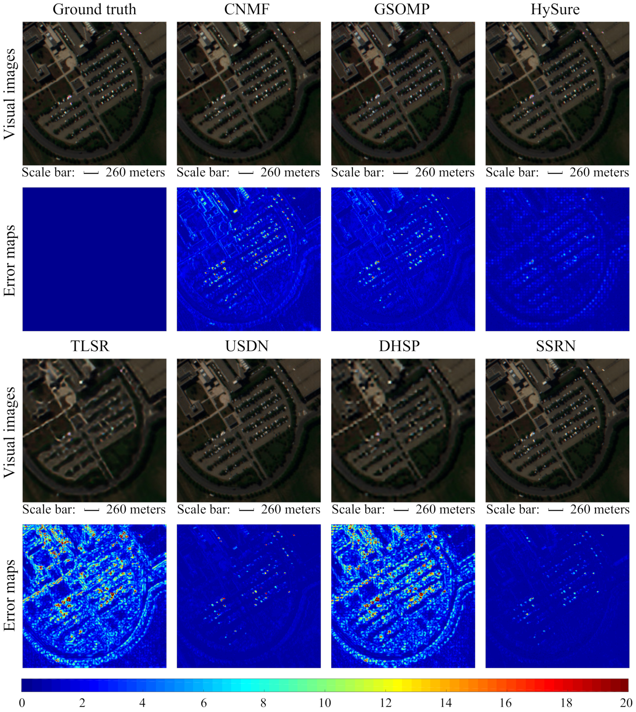
To visualize the experimental results, the visual images and error maps of SSRN and the compared methods are displayed in Figure 4. The HSIs estimated by TLSR and DHSP are blurry, since TLSR and DHSP cannot utilize the spatial information of the MSI. In the estimated HSIs of TLSR and DHSP, the small targets that only cover one or two pixels are missing. As shown in the error maps, the proposed SSRN effectively preserves the spatial structures of the estimated HSI.

4.3.2. WDCM Database

The quantitative results of SSRN and the compared methods on the WDCM database are reported in Table 6. CNMF, GSOMP, and HySure show better performance than TLSR and DHSP, since the spatial information of the MSI is utilized. The performance of USDN can compete with CNMF, GSOMP, and HySure. As shown in Table 6, the performance of the proposed SSRN is better than the compared methods in terms of PSNR, RMSE, and SAM. In terms of UIQI and ERGAS, the proposed SSRN shows favorable performance, which is close to the results of GSOMP.
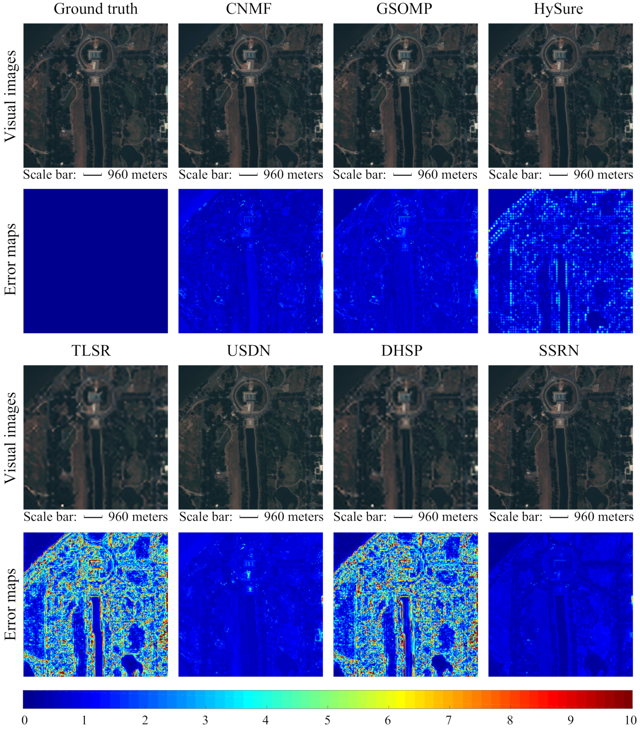
Visual images and error maps of SSRN and the compared methods on the WDCM database are shown in Figure 5. The visual images of CNMF, GSOMP, HySure, USDN, and the proposed SSRN have good visualization results, owing to the reliable spatial information provided by the HR MSI. As shown in the error maps, the errors of TLSR and DHSP are mainly concentrated on the edges of complicated land-covers. The proposed SSRN shows superior performance in complicated land-covers.

4.4. Comparisons with Other Methods on Real Databases

In this subsection, SSRN and the compared methods are evaluated on two real databases. On the Paris and Ivanpah Playa databases, the number of training epochs is set as 400 for SSRN. The learning rate of SSRN is initially set as 0.01, which then drops by a factor of 10 after 200 epochs.

4.4.1. Paris Database

On the Paris database, HR MSIs and LR HSIs are captured at the same time instant. On this database, the LR HSI is generated from the original HSI for training. After spatially downsampling with the scaling factor of 4, the LR HSI contains only 18 × 18 pixels, which is far less than the number of pixels on simulated databases. Insufficient pixels in the LR HSI can make the proposed SSRN difficult to train. To alleviate the problem of insufficient pixels, the training samples are flipped left and right. Furthermore, the training samples are rotated 90, 180, and 270 degrees. On the Paris database, the spectral response function is estimated with the method proposed in the literature [12]. The performance of SSRN and the compared methods on the Paris database is shown in Table 7. In comparison with the PU and WDCM databases, the performance of SSRN and the compared methods decreased due to the too complicated land-cover distributions on the Paris database. As shown in Table 7, the proposed SSRN still shows better performance than the compared methods.
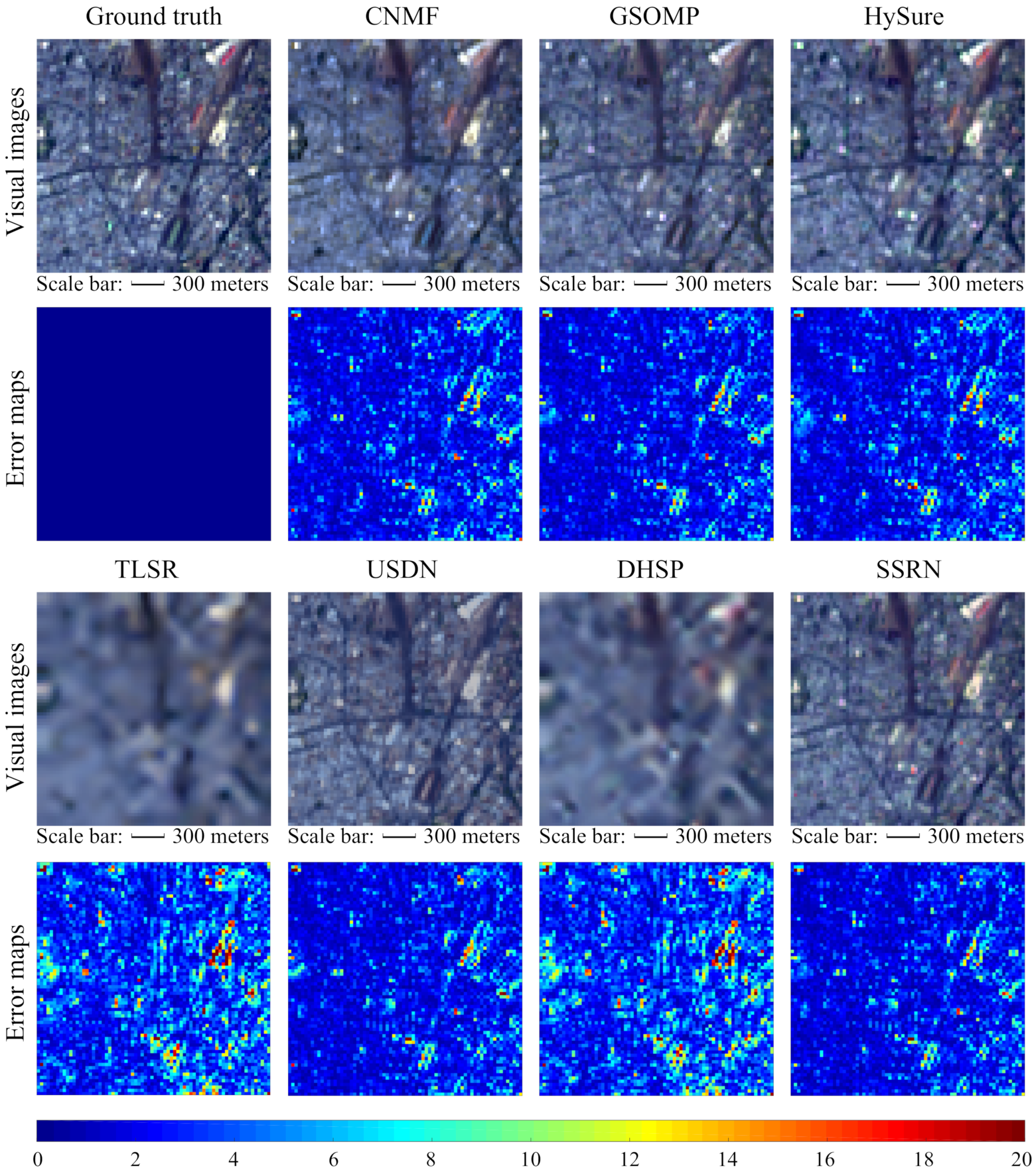
Visual images and error maps of SSRN and the compared methods are shown in Figure 6. Since the proposed SSRN estimates the HSI directly from the MSI, the spatial information of the MSI can be fully utilized. As shown in Figure 6, compared to the error maps of other methods, the proposed SSRN effectively mitigates the spatial distortion.

4.4.2. Ivanpah Playa Database

The Ivanpah Playa database is a real database that consists of a LR HSI collected on 26 October 2015 and a HR MSI captured on 17 December 2017. On the Ivanpah Playa database, the HR MSI and LR HSI are collected during different seasons. In practice, seasonal changes may result in that the same land-cover material having different intrinsic spectral signatures [1]. Therefore, the intrinsic spectral signatures of the same land-cover may be different in LR MSIs and HR HSIs on the Ivanpah Playa database. It is challenging to perform HR MSI and LR HSI fusion on the Ivanpah Playa database. On this database, similar to the literature [1], the spectral response function from calibration measurements (https://earth.esa.int/web/sentinel/user-guides/sentinel-2-msi/document-library/-/asset_publisher/Wk0TKajiISaR/content/sentinel-2aspectral-responses, accessed on 17 December 2020) is employed for the compared methods.
Experimental results of SSRN and the compared methods on the Ivanpah Playa database are reported in Table 8. Different from that on the PU, WDCM, and Paris databases, TLSR and DHSP perform better than traditional methods and USDN on the Ivanpah Playa database. CNMF, GSOMP, HySure, and USDN usually rely on the assumption that the intrinsic spectral signatures of the same land-cover in HR MSIs and LR HSIs are the same [28,36]. In these methods, the spectral response function is usually directly used to obtain the spectral ingredients of HR MSIs from the spectral ingredients of LR HSIs. However, this assumption is not satisfied on the Ivanpah Playa database, which results in the performance degradations of CNMF, GSOMP, HySure, and USDN.
Different from CNMF, GSOMP, HySure, and USDN, the proposed SSRN does not rely on the assumption that the intrinsic spectral signatures of the same land-cover in HR MSIs and LR HSIs are the same. In the proposed SSRN, the fusion problem of the HR MSI and the LR HSI is considered a problem of spectral mapping learning. The proposed SSRN is utilized to directly learn spectral mapping from the multispectral pixels to the hyperspectral pixels. Owing to the powerful nonlinear representation ability of deep convolutional networks, SSRN can model the spectral variability increased by the seasonal changes between multispectral and hyperspectral pixels. In addition, due to HR MSI and LR HSI on the Ivanpah Playa database being collected at different time instants, the imaging environments (e.g., illumination, atmospheric, and weather) of HR MSIs and LR HSIs are different. Different imaging environments may result in it being difficult to accurately obtain real spectral response function [12]. In the proposed SSRN, only the loss function requires a spectral response function. To reduce the errors caused by the estimated spectral response function, the second term in the loss function Equation (9) and the fine-tuning strategy of SSRN are removed in the experiments on the Ivanpah Playa database. Data augmentation that is same as that on the Paris database is also employed on the Ivanpah Playa database to increase the number of training samples. As shown in Table 8, in terms of PSNR, UIQI, RMSE, and ERGAS, the proposed SSRN shows superior performance.
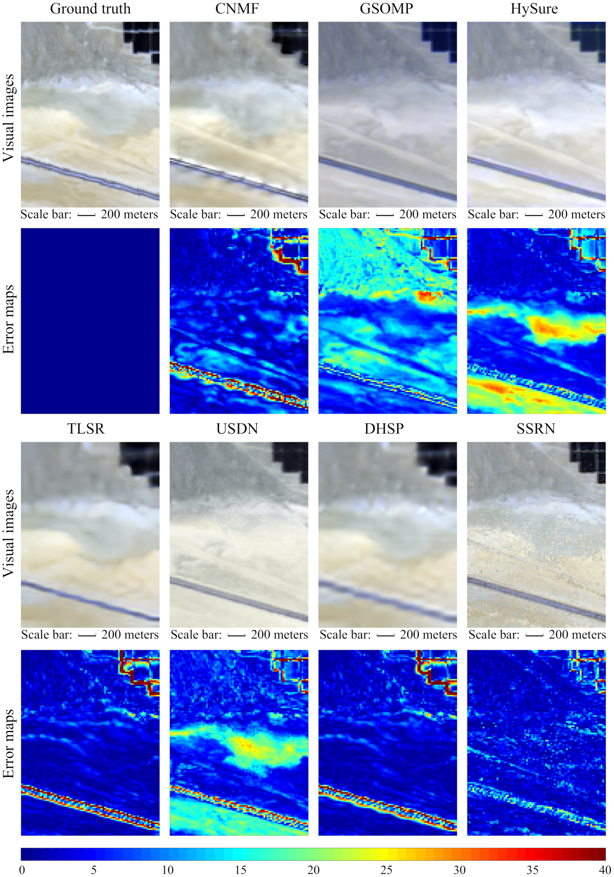
Visual images and error maps are shown in Figure 7. The spatial structures on the Ivanpah Playa database are relatively smooth. Although TLSR and DHSP cause the high-frequency information of the reconstructed image to be blurred, the experimental results of TLSR and DHSP in the smooth land-cover regions are favorable. According to the visual image and the error map of SSRN, the proposed SSRN effectively preserves the spatial structures of the HR MSI in the estimated HSI.

4.5. Time Cost

The total time cost of SSRN and the compared methods on the PU, WDCM, Paris, and Playa databases is shown in Table 9. In this paper, all experiments are conducted on the Ubuntu 14.04 system, 64G RAM, Intel Core i7-5930K, and NVIDIA TITAN X. CNMF, GSOMP, HySure, and TLSR are implemented with MATLAB. DHSP is implemented with PyTorch. USDN and the proposed SSRN are implemented with TensorFlow. The codes ofthe traditional methods (CNMF, GSOMP, and HySure) are implemented with the CPU. In the compared methods, the DL-based methods include TLSR, USDN, and DHSP. However, the code of TLSR provided by the original literature [26] is implemented with the CPU rather than the GPU. The codes of other deep learning-based methods (USDN, DHSP, and the proposed SSRN) are implemented with the GPU. As shown in Table 9, CNMF has superior computational efficiency. In general, DL-based methods usually take more time than traditional methods due to plenty of weight parameters. In the training process, the inputs of the proposed SSRN are image patches and the inputs of TLSR, USDN, and DHSP are entire images. Therefore, the proposed SSRN has less time cost than TLSR, USDN, and DHSP.

5. Discussion

The performance of the proposed SSRN heavily depends on the learning of the spectral mapping. When the spectral information contained in MSI is too little, it becomea difficult to learn effective spectral mapping, which may weaken the performance of the proposed SSRN. For instance, RGB images (special MSIs), containing only three spectral bands, have little spectral information. Similar colors in RGB images may represent different objects. In other words, similar RGB image pixels may correspond to different HSI pixels, which makes it challenging to learn the spectral mapping between MSIs and HSIs. In this subsection, to explore the performance of SSRN when the MSI contains little spectral information, the CAVE database [55] is employed to conducted experiments. The average quantitative results are reported in Table 10. On the CAVE database, the MSI only contains three spectral bands, making it challenging to learn the spectral mapping between MSIs and HSIs. In terms of PSNR, UIQI, RMSE, and ERGAS, the performance of SSRN is weaker than that of CNMF and HySure. In terms of SAM, the proposed SSRN outperforms the compared methods.

6. Conclusions

In this paper, a spectral-spatial residual network is proposed to estimate HR HSI based on the observed HR MSI and LR HSI. Different from previous methods that focus on extracting spectral ingredients from LR HSI and extracting spatial ingredients from HR MSI, the proposed SSRN directly learns pixel-wise spectral mapping between MSIs and HSIs. In SSRN, a spectral module is proposed to extract spectral features from MSIs and a spatial module is proposed to explore the complementarity of homogeneous adjacent pixels to facilitate learning of spectral mapping. Finally, a self-supervised fine-tuning strategy is proposed to estimate the spectral mapping between HR MSIs and HR HSIs on the basis of the learned pixel-wise spectral mapping between LR MSIs and LR HSIs. Experiments on simulated and real databases show that SSRN can effectively reduce spatial and spectral distortions and can achieve superior performance. In the future, we will study more efficient deep networks for learning spectral mapping between MSIs and HSIs.

Author Contributions

Conceptualization, W.C. and X.Z.; methodology, W.C.; software, W.C.; validation, W.C., X.Z., and X.L.; formal analysis, X.Z.; investigation, W.C.; resources, X.Z.; data curation, W.C.; writing—original draft preparation, W.C.; writing—review and editing, X.Z.; visualization, X.Z.; supervision, X.L.; project administration, X.L.; funding acquisition, X.L. All authors have read and agreed to the published version of the manuscript.

Funding

This work was funded in part by the National Science Fund for Distinguished Young Scholars under grant 61925112, in part by the National Natural Science Foundation of China under grant 61806193 and grant 61772510, in part by the Innovation Capability Support Program of Shaanxi under grant 2020KJXX-091 and grant 2020TD-015, and in part by the Natural Science Basic Research Program of Shaanxi under grants 2019JQ-340 and 2019JC-23.

Institutional Review Board Statement

Not applicable.

Informed Consent Statement

Not applicable.

Data Availability Statement

Not applicable.

Acknowledgments

The authors would like to thank the editors and reviewers for their insightful suggestions.

Conflicts of Interest

The authors declare no conflict of interest.

References

  1. Borsoi, R.A.; Imbiriba, T.; Bermudez, J.C.M. Super-Resolution for Hyperspectral and Multispectral Image Fusion Accounting for Seasonal Spectral Variability. IEEE Trans. Image Process. 2020, 29, 116–127. [Google Scholar] [CrossRef] [PubMed] [Green Version]
  2. Sun, H.; Zheng, X.; Lu, X.; Wu, S. Spectral-Spatial Attention Network for Hyperspectral Image Classification. IEEE Trans. Geosci. Remote Sens. 2020, 58, 3232–3245. [Google Scholar] [CrossRef]
  3. Zhao, X.; Li, W.; Zhang, M.; Tao, R.; Ma, P. Adaptive Iterated Shrinkage Thresholding-Based Lp-Norm Sparse Representation for Hyperspectral Imagery Target Detection. Remote Sens. 2020, 12, 3991. [Google Scholar] [CrossRef]
  4. Ren, X.; Lu, L.; Chanussot, J. Toward Super-Resolution Image Construction Based on Joint Tensor Decomposition. Remote Sens. 2020, 12, 2535. [Google Scholar] [CrossRef]
  5. Zhang, K.; Wang, M.; Yang, S. Multispectral and Hyperspectral Image Fusion Based on Group Spectral Embedding and Low-Rank Factorization. IEEE Trans. Geosci. Remote Sens. 2017, 55, 1363–1371. [Google Scholar] [CrossRef]
  6. Chen, W.; Lu, X. Unregistered Hyperspectral and Multispectral Image Fusion with Synchronous Nonnegative Matrix Factorization. In Chinese Conference on Pattern Recognition and Computer Vision, Proceedings of the Third Chinese Conference, PRCV 2020, Nanjing, China, 16–18 October 2020; Springer: Berlin/Heidelberg, Germany, 2020; pp. 602–614. [Google Scholar]
  7. Liu, W.; Lee, J. An Efficient Residual Learning Neural Network for Hyperspectral Image Superresolution. IEEE J. Sel. Top. Appl. Earth Obs. Remote Sens. 2019, 12, 1240–1253. [Google Scholar] [CrossRef]
  8. Loncan, L.; de Almeida, L.B.; Bioucas-Dias, J.M.; Briottet, X.; Chanussot, J.; Dobigeon, N.; Fabre, S.; Liao, W.; Licciardi, G.A.; Simões, M.; et al. Hyperspectral Pansharpening: A Review. IEEE Geosci. Remote Sens. Mag. 2015, 3, 27–46. [Google Scholar] [CrossRef] [Green Version]
  9. Yokoya, N.; Grohnfeldt, C.; Chanussot, J. Hyperspectral and Multispectral Data Fusion: A comparative review of the recent literature. IEEE Geosci. Remote Sens. Mag. 2017, 5, 29–56. [Google Scholar] [CrossRef]
  10. Han, X.; Shi, B.; Zheng, Y. Self-Similarity Constrained Sparse Representation for Hyperspectral Image Super-Resolution. IEEE Trans. Image Process. 2018, 27, 5625–5637. [Google Scholar] [CrossRef]
  11. Feng, X.; He, L.; Cheng, Q.; Long, X.; Yuan, Y. Hyperspectral and Multispectral Remote Sensing Image Fusion Based on Endmember Spatial Information. Remote Sens. 2020, 12, 1009. [Google Scholar] [CrossRef] [Green Version]
  12. Simões, M.; Bioucas-Dias, J.; Almeida, L.B.; Chanussot, J. A Convex Formulation for Hyperspectral Image Superresolution via Subspace-Based Regularization. IEEE Trans. Geosci. Remote Sens. 2015, 53, 3373–3388. [Google Scholar] [CrossRef] [Green Version]
  13. Wei, Q.; Dobigeon, N.; Tourneret, J. Fast Fusion of Multi-Band Images Based on Solving a Sylvester Equation. IEEE Trans. Image Process. 2015, 24, 4109–4121. [Google Scholar] [CrossRef] [Green Version]
  14. Zhou, Y.; Feng, L.; Hou, C.; Kung, S. Hyperspectral and Multispectral Image Fusion Based on Local Low Rank and Coupled Spectral Unmixing. IEEE Trans. Geosci. Remote Sens. 2017, 55, 5997–6009. [Google Scholar] [CrossRef]
  15. Zhang, K.; Wang, M.; Yang, S.; Jiao, L. Spatial-Spectral-Graph-Regularized Low-Rank Tensor Decomposition for Multispectral and Hyperspectral Image Fusion. IEEE J. Sel. Top. Appl. Earth Obs. Remote Sens. 2018, 11, 1030–1040. [Google Scholar] [CrossRef]
  16. Dian, R.; Li, S.; Fang, L.; Lu, T.; Bioucas-Dias, J.M. Nonlocal Sparse Tensor Factorization for Semiblind Hyperspectral and Multispectral Image Fusion. IEEE Trans. Cybern. 2020, 50, 4469–4480. [Google Scholar] [CrossRef]
  17. Ma, J.; Yu, W.; Chen, C.; Liang, P.; Guo, X.; Jiang, J. Pan-GAN: An unsupervised pan-sharpening method for remote sensing image fusion. Inf. Fusion 2020, 62, 110–120. [Google Scholar] [CrossRef]
  18. Zhang, L.; Nie, J.; Wei, W.; Zhang, Y.; Liao, S.; Shao, L. Unsupervised Adaptation Learning for Hyperspectral Imagery Super-Resolution. In Proceedings of the IEEE/CVF Conference on Computer Vision and Pattern Recognition (CVPR), Seattle, WA, USA, 14–19 June 2020; pp. 3070–3079. [Google Scholar] [CrossRef]
  19. Zhang, X.; Huang, W.; Wang, Q.; Li, X. SSR-NET: Spatial-Spectral Reconstruction Network for Hyperspectral and Multispectral Image Fusion. IEEE Trans. Geosci. Remote Sens. 2020, 1–13. [Google Scholar] [CrossRef]
  20. Xie, Q.; Zhou, M.; Zhao, Q.; Meng, D.; Zuo, W.; Xu, Z. Multispectral and Hyperspectral Image Fusion by MS/HS Fusion Net. In Proceedings of the IEEE/CVF Conference on Computer Vision and Pattern Recognition (CVPR), Long Beach, CA, USA, 16–20 June 2019; pp. 1585–1594. [Google Scholar] [CrossRef] [Green Version]
  21. Dian, R.; Li, S.; Guo, A.; Fang, L. Deep Hyperspectral Image Sharpening. IEEE Trans. Neural Netw. Learn. Syst. 2018, 29, 5345–5355. [Google Scholar] [CrossRef]
  22. Xie, W.; Jia, X.; Li, Y.; Lei, J. Hyperspectral Image Super-Resolution Using Deep Feature Matrix Factorization. IEEE Trans. Geosci. Remote Sens. 2019, 57, 6055–6067. [Google Scholar] [CrossRef]
  23. Wei, Y.; Yuan, Q.; Shen, H.; Zhang, L. Boosting the Accuracy of Multispectral Image Pansharpening by Learning a Deep Residual Network. IEEE Geosci. Remote Sens. Lett. 2017, 14, 1795–1799. [Google Scholar] [CrossRef] [Green Version]
  24. Wang, W.; Zeng, W.; Huang, Y.; Ding, X.; Paisley, J. Deep Blind Hyperspectral Image Fusion. In Proceedings of the IEEE/CVF International Conference on Computer Vision (ICCV), Long Beach, CA, USA, 16–20 June 2019; pp. 4149–4158. [Google Scholar] [CrossRef]
  25. Li, K.; Xie, W.; Du, Q.; Li, Y. DDLPS: Detail-Based Deep Laplacian Pansharpening for Hyperspectral Imagery. IEEE Trans. Geosci. Remote Sens. 2019, 57, 8011–8025. [Google Scholar] [CrossRef]
  26. Yuan, Y.; Zheng, X.; Lu, X. Hyperspectral Image Superresolution by Transfer Learning. IEEE J. Sel. Top. Appl. Earth Obs. Remote Sens. 2017, 10, 1963–1974. [Google Scholar] [CrossRef]
  27. Sidorov, O.; Hardeberg, J.Y. Deep Hyperspectral Prior: Single-Image Denoising, Inpainting, Super-Resolution. In Proceedings of the IEEE/CVF International Conference on Computer Vision (ICCV), Long Beach, CA, USA, 16–20 June 2019; pp. 3844–3851. [Google Scholar] [CrossRef]
  28. Qu, Y.; Qi, H.; Kwan, C. Unsupervised Sparse Dirichlet-Net for Hyperspectral Image Super-Resolution. In Proceedings of the IEEE/CVF Conference on Computer Vision and Pattern Recognition, Salt Lake City, UT, USA, 18–23 June 2018; pp. 2511–2520. [Google Scholar] [CrossRef] [Green Version]
  29. Fang, L.; Zhuo, H.; Li, S. Super-resolution of hyperspectral image via superpixel-based sparse representation. Neurocomputing 2018, 273, 171–177. [Google Scholar] [CrossRef]
  30. Akhtar, N.; Shafait, F.; Mian, A. Sparse Spatio-spectral Representation for Hyperspectral Image Super-resolution. In European Conference on Computer Vision, Proceedings of the Computer Vision—ECCV 2014, Zurich, Switzerland, 6–12 September 2014; Springer International Publishing: Cham, Switzerland, 2014; pp. 63–78. [Google Scholar]
  31. Wei, Q.; Bioucas-Dias, J.; Dobigeon, N.; Tourneret, J. Hyperspectral and Multispectral Image Fusion Based on a Sparse Representation. IEEE Trans. Geosci. Remote Sens. 2015, 53, 3658–3668. [Google Scholar] [CrossRef] [Green Version]
  32. Wei, Q.; Dobigeon, N.; Tourneret, J. Bayesian fusion of hyperspectral and multispectral images. In Proceedings of the IEEE International Conference on Acoustics, Speech and Signal Processing (ICASSP), Florence, Italy, 4–9 May 2014; pp. 3176–3180. [Google Scholar] [CrossRef] [Green Version]
  33. Eismann, M.T.; Hardie, R.C. Hyperspectral resolution enhancement using high-resolution multispectral imagery with arbitrary response functions. IEEE Trans. Geosci. Remote Sens. 2005, 43, 455–465. [Google Scholar] [CrossRef]
  34. Wei, Q.; Dobigeon, N.; Tourneret, J. Bayesian Fusion of Multi-Band Images. IEEE J. Sel. Top. Signal Process. 2015, 9, 1117–1127. [Google Scholar] [CrossRef] [Green Version]
  35. Irmak, H.; Akar, G.B.; Yuksel, S.E. A MAP-Based Approach for Hyperspectral Imagery Super-Resolution. IEEE Trans. Image Process. 2018, 27, 2942–2951. [Google Scholar] [CrossRef]
  36. Yokoya, N.; Yairi, T.; Iwasaki, A. Coupled Nonnegative Matrix Factorization Unmixing for Hyperspectral and Multispectral Data Fusion. IEEE Trans. Geosci. Remote Sens. 2012, 50, 528–537. [Google Scholar] [CrossRef]
  37. Lin, C.; Ma, F.; Chi, C.; Hsieh, C. A Convex Optimization-Based Coupled Nonnegative Matrix Factorization Algorithm for Hyperspectral and Multispectral Data Fusion. IEEE Trans. Geosci. Remote Sens. 2018, 56, 1652–1667. [Google Scholar] [CrossRef]
  38. Li, S.; Dian, R.; Fang, L.; Bioucas-Dias, J.M. Fusing Hyperspectral and Multispectral Images via Coupled Sparse Tensor Factorization. IEEE Trans. Image Process. 2018, 27, 4118–4130. [Google Scholar] [CrossRef] [PubMed]
  39. Li, J.; Cui, R.; Li, B.; Song, R.; Li, Y.; Du, Q. Hyperspectral Image Super-Resolution with 1D-2D Attentional Convolutional Neural Network. Remote Sens. 2019, 11, 2859. [Google Scholar] [CrossRef] [Green Version]
  40. Fu, Y.; Zhang, T.; Zheng, Y.; Zhang, D.; Huang, H. Hyperspectral Image Super-Resolution with Optimized RGB Guidance. In Proceedings of the IEEE/CVF Conference on Computer Vision and Pattern Recognition (CVPR), Long Beach, CA, USA, 16–20 June 2019; pp. 11653–11662. [Google Scholar] [CrossRef]
  41. Wang, Z.; Chen, B.; Lu, R.; Zhang, H.; Liu, H.; Varshney, P.K. FusionNet: An Unsupervised Convolutional Variational Network for Hyperspectral and Multispectral Image Fusion. IEEE Trans. Image Process. 2020, 29, 7565–7577. [Google Scholar] [CrossRef]
  42. Huang, W.; Xiao, L.; Wei, Z.; Liu, H.; Tang, S. A New Pan-Sharpening Method with Deep Neural Networks. IEEE Geosci. Remote Sens. Lett. 2015, 12, 1037–1041. [Google Scholar] [CrossRef]
  43. Li, J.; Wu, C.; Song, R.; Xie, W.; Ge, C.; Li, B.; Li, Y. Hybrid 2-D-3-D Deep Residual Attentional Network with Structure Tensor Constraints for Spectral Super-Resolution of RGB Images. IEEE Trans. Geosci. Remote Sens. 2020, 1–15. [Google Scholar] [CrossRef]
  44. Fu, Y.; Zhang, T.; Zheng, Y.; Zhang, D.; Huang, H. Joint Camera Spectral Response Selection and Hyperspectral Image Recovery. IEEE Trans. Pattern Anal. Mach. Intell. 2020. [Google Scholar] [CrossRef]
  45. Akhtar, N.; Mian, A. Hyperspectral Recovery from RGB Images using Gaussian Processes. IEEE Trans. Pattern Anal. Mach. Intell. 2020, 42, 100–113. [Google Scholar] [CrossRef] [Green Version]
  46. Yan, L.; Wang, X.; Zhao, M.; Kaloorazi, M.; Chen, J.; Rahardja, S. Reconstruction of Hyperspectral Data from RGB Images with Prior Category Information. IEEE Trans. Comput. Imaging 2020, 6, 1070–1081. [Google Scholar] [CrossRef]
  47. He, K.; Zhang, X.; Ren, S.; Sun, J. Deep Residual Learning for Image Recognition. In Proceedings of the IEEE Conference on Computer Vision and Pattern Recognition (CVPR), Las Vegas, NV, USA, 27–30 June 2016; pp. 770–778. [Google Scholar] [CrossRef] [Green Version]
  48. Song, W.; Li, S.; Fang, L.; Lu, T. Hyperspectral Image Classification with Deep Feature Fusion Network. IEEE Trans. Geosci. Remote Sens. 2018, 56, 3173–3184. [Google Scholar] [CrossRef]
  49. Sun, H.; Li, S.; Zheng, X.; Lu, X. Remote Sensing Scene Classification by Gated Bidirectional Network. IEEE Trans. Geosci. Remote Sens. 2020, 58, 82–96. [Google Scholar] [CrossRef]
  50. Sun, H.; Zheng, X.; Lu, X. A Supervised Segmentation Network for Hyperspectral Image Classification. IEEE Trans. Image Process. 2021, 30, 2810–2825. [Google Scholar] [CrossRef]
  51. Lu, X.; Dong, L.; Yuan, Y. Subspace Clustering Constrained Sparse NMF for Hyperspectral Unmixing. IEEE Trans. Geosci. Remote Sens. 2020, 58, 3007–3019. [Google Scholar] [CrossRef]
  52. Du, X.; Zheng, X.; Lu, X.; Doudkin, A.A. Multisource Remote Sensing Data Classification with Graph Fusion Network. IEEE Trans. Geosci. Remote Sens. 2021, 1–11. [Google Scholar] [CrossRef]
  53. Dian, R.; Li, S. Hyperspectral Image Super-Resolution via Subspace-Based Low Tensor Multi-Rank Regularization. IEEE Trans. Image Process. 2019, 28, 5135–5146. [Google Scholar] [CrossRef]
  54. Wang, X.; Girshick, R.; Gupta, A.; He, K. Non-local Neural Networks. In Proceedings of the IEEE/CVF Conference on Computer Vision and Pattern Recognition, Salt Lake City, UT, USA, 18–23 June 2018; pp. 7794–7803. [Google Scholar] [CrossRef] [Green Version]
  55. Yasuma, F.; Mitsunaga, T.; Iso, D.; Nayar, S.K. Generalized Assorted Pixel Camera: Postcapture Control of Resolution, Dynamic Range, and Spectrum. IEEE Trans. Image Process. 2010, 19, 2241–2253. [Google Scholar] [CrossRef] [Green Version]
  56. Akhtar, N.; Shafait, F.; Mian, A. Bayesian sparse representation for hyperspectral image super resolution. In Proceedings of the IEEE Conference on Computer Vision and Pattern Recognition (CVPR), Boston, MA, USA, 7–12 June 2015; pp. 3631–3640. [Google Scholar] [CrossRef]
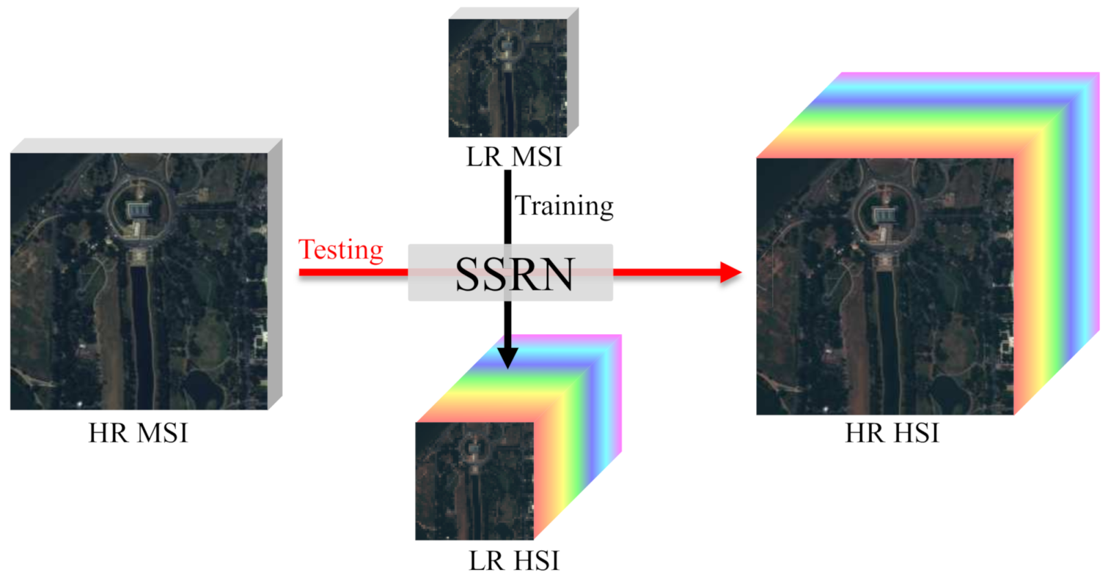
Figure 1. Illustration of the proposed spectral-spatial residual network (SSRN) framework. Firstly, a low spatial resolution (LR) multispectral image (MSI) and an LR hyperspectral image (HSI) are utilized to train the proposed SSRN to learn the pixel-wise spectral mapping. Then, the learned pixel-wise spectral mapping is exploited to estimate high spatial resolution (HR) HSIs from HR MSIs.
Remotesensing 13 01260 g001
Figure 2. Architecture of the proposed SSRN. A spectral module and a spatial module are utilized to learn the pixel-wise spectral mapping between MSIs and HSIs. ⊕ represents the residual connection.
Remotesensing 13 01260 g002
Figure 3. Structures of the residual block and the self-attention module. ⊕ represents the residual connection. ReLU represents the rectified linear unit.
Remotesensing 13 01260 g003
Figure 4. Visual images (R: 60, G: 30, and B: 10) and error maps of SSRN and the compared methods on the PU database. The error maps are the sum of absolute differences in all spectral bands between the estimated HSI and the ground truth.
Remotesensing 13 01260 g004
Figure 5. Visual images (R: 50, G: 30, and B: 20) and error maps of SSRN and the compared methods on the WDCM database.
Remotesensing 13 01260 g005
Figure 6. Visual images (R: 24, G: 14, and B: 3) and error maps of the proposed SSRN and the compared methods on the Paris database.
Remotesensing 13 01260 g006
Figure 7. Visual images (R: 32, G: 20, and B: 8) and error maps of the proposed SSRN and the compared methods on the Ivanpah Playa database.
Remotesensing 13 01260 g007
Table 1. Peak signal-to-noise ratio (PSNR) and spectral angle mapper (SAM) of SSRN with different numbers of convolutional kernels on the Washington DC Mall (WDCM) database.
Number163264128256512
PSNR31.77232.47732.92633.04433.12333.048
SAM1.4851.3851.2871.2451.2281.245
Table 2. PSNR and SAM of SSRN with different numbers of residual blocks on the WDCM database.
Number123456
PSNR32.85033.14933.12333.16732.97832.941
SAM1.2321.2151.2281.2131.2191.240
Table 3. PSNR and SAM of SSRN with different λ on the WDCM database.
λ 0.0010.010.11510
PSNR31.95932.47333.16733.06031.88429.940
SAM1.4361.4111.2131.2441.2541.267
Table 4. Ablation experiments of SSRN on the WDCM databases.
Ablation Study
MLFA×
Spatial module××
Cosine similarity loss×××
Fine-tuning××××
PSNR31.90232.06132.15033.16733.232
SAM1.5141.4821.4941.2131.211
1. × represents that the basic network is configured with the component. 2. √ represents that the basic network is not configured with the component.
Table 5. Quantitative experimental results on the Pavia University (PU) database.
MethodsPSNRUIQIRMSEERGASSAM
CNMF [36]33.0720.9635.8283.6543.710
GSOMP [30]35.1170.9714.8193.2304.050
HySure [12]38.7100.9833.2262.0373.453
TLSR [26]25.3490.78314.0938.6256.815
USDN [28]36.9440.9773.8352.6203.340
DHSP [27]25.7020.79913.5048.2826.606
SSRN39.7410.9852.8861.9802.781
Table 6. Quantitative experimental results on the WDCM database.
MethodsPSNRUIQIRMSEERGASSAM
CNMF [36]32.2170.9481.52074.1971.944
GSOMP [30]31.9790.9561.72957.5871.877
HySure [12]30.4840.9402.31659.7992.518
TLSR [26]21.6630.7128.59561.6636.095
USDN [28]31.3550.9351.805122.3362.264
DHSP [27]21.9170.7498.566122.0695.967
SSRN33.2320.9541.44861.2161.211
Table 7. Quantitative experimental results on the Paris database.
MethodsPSNRUIQIRMSEERGASSAM
CNMF [36]27.8790.8197.5643.6013.534
GSOMP [30]28.2350.8177.2993.5173.381
HySure [12]27.6210.8247.8863.7633.759
TLSR [26]24.6710.52010.9855.1304.806
USDN [28]27.9750.8037.5093.6223.435
DHSP [27]24.5690.51611.1065.1854.935
SSRN28.3500.8297.1853.4343.334
Table 8. Quantitative experimental results on the Ivanpah Playa database.
MethodsPSNRUIQIRMSEERGASSAM
CNMF [36]23.3990.72115.6002.3951.456
GSOMP [30]20.8550.48121.7033.2953.575
HySure [12]21.6580.53119.1262.9392.221
TLSR [26]23.7020.78615.1492.3301.440
USDN [28]22.1430.48718.0482.7692.169
DHSP [27]23.9630.79214.6722.2571.418
SSRN27.7700.8079.4471.4511.451
Table 9. Time cost of different methods on different databases (seconds).
MethodsCPU/GPUPUWDCMParisPlaya
CNMF [36]CPU12.3714.261.563.64
GSOMP [30]CPU77.60160.7010.5920.52
HySure [12]CPU40.9658.736.8526.21
TLSR [26]CPU1130.83541.05251.68492.56
USDN [28]GPU782.65198.68151.53134.43
DHSP [27]GPU796.921885.74259.89470.56
SSRNGPU74.09117.2182.88181.46
Table 10. Quantitative experimental results on the CAVE database.
MethodsPSNRUIQIRMSEERGASSAM
CNMF [36]42.4030.8452.2732.3376.629
GSOMP [30]37.2040.8245.1225.43912.556
HySure [12]41.3310.8142.1302.5306.645
TLSR [26]34.1480.7445.2065.8796.221
USDN [28]37.7110.8253.7693.84711.493
DHSP [27]34.2050.7035.1905.8407.096
SSRN40.5580.8162.5203.0315.523
Publisher’s Note: MDPI stays neutral with regard to jurisdictional claims in published maps and institutional affiliations.