Abstract
The net ecosystem CO2 exchange (NEE) is a critical parameter for quantifying terrestrial ecosystems and their contributions to the ongoing climate change. The accumulation of ecological data is calling for more advanced quantitative approaches for assisting NEE prediction. In this study, we applied two widely used machine learning algorithms, Random Forest (RF) and Extreme Gradient Boosting (XGBoost), to build models for simulating NEE in major biomes based on the FLUXNET dataset. Both models accurately predicted NEE in all biomes, while XGBoost had higher computational efficiency (6~62 times faster than RF). Among environmental variables, net solar radiation, soil water content, and soil temperature are the most important variables, while precipitation and wind speed are less important variables in simulating temporal variations of site-level NEE as shown by both models. Both models perform consistently well for extreme climate conditions. Extreme heat and dryness led to much worse model performance in grassland (extreme heat: R2 = 0.66~0.71, normal: R2 = 0.78~0.81; extreme dryness: R2 = 0.14~0.30, normal: R2 = 0.54~0.55), but the impact on forest is less (extreme heat: R2 = 0.50~0.78, normal: R2 = 0.59~0.87; extreme dryness: R2 = 0.86~0.90, normal: R2 = 0.81~0.85). Extreme wet condition did not change model performance in forest ecosystems (with R2 changing −0.03~0.03 compared with normal) but led to substantial reduction in model performance in cropland (with R2 decreasing 0.20~0.27 compared with normal). Extreme cold condition did not lead to much changes in model performance in forest and woody savannas (with R2 decreasing 0.01~0.08 and 0.09 compared with normal, respectively). Our study showed that both models need training samples at daily timesteps of >2.5 years to reach a good model performance and >5.4 years of daily samples to reach an optimal model performance. In summary, both RF and XGBoost are applicable machine learning algorithms for predicting ecosystem NEE, and XGBoost algorithm is more feasible than RF in terms of accuracy and efficiency.
1. Introduction
The biosphere acts as an important regulator for the global climate system through land-atmosphere exchange of greenhouse gases [1,2,3], of which the net ecosystem CO2 exchange (NEE) is arguably one of the most critical components [4]. The NEE has been widely measured by eddy covariance (EC) techniques [5,6]. The EC technique uses classical micrometeorological principles to compute the covariance between the vertical velocity, CO2, and water vapor concentration pulsations, and thus can directly measure the net CO2 exchange between the canopy and the atmosphere [7]. The footprint of the EC tower varies from meters to hundreds of meters, depending on the height of the tower and spatial heterogeneity of vegetation. Hundreds of EC tower sites have been operating worldwide, most of which contribute data to FLUXNET datasets [6,8].
Across the globe, the large amount of EC datasets enables upscaling NEE prediction from site to regional scale, primarily based on process-based models [9,10,11,12,13] and data-oriented approaches [14,15]. Process-based ecosystem models can be used for evaluating spatiotemporal patterns and trends of the carbon cycle in terrestrial ecosystems [16,17,18,19]. However, there are uncertainties in the description of certain mechanisms, and different parameters have significant impacts on the simulation results [13]. Additionally, all the models rely on different datasets and intensive computational cost. Data-oriented approaches are the complements to process-based models, and their algorithms and tools are critically important for the robustness of the approaches.
Machine learning (ML) methods have been widely adopted in investigating land cover change [20], environmental monitoring [21], carbon flux assessment [22], water resource monitoring [23], and gap-filling for eddy covariance dataset [24]. The ML algorithms use an advanced statistical approach to extract critical information contained in large datasets without explicit instructions [25]. Artificial neural network (ANN), supports vector machines for regression (SVR), and tree-based model (e.g., regression tree, model tree ensembles, random forest, and gradient boosting regression) are three widely used approaches for NEE prediction. Some novel algorithms such as deep learning [26] and symbolic regression [27,28] also offer the possibility of NEE prediction. The ANN algorithm has been used for CO2 flux prediction in different ecosystems over the past 20 years [29,30,31]. More recent studies [32,33] combined ANN with SVR [34] to develop gross primary productivity (GPP) and NEE databases at site-level and continental-scale with EC data and remote sensing datasets. Tree-based models are the other type of ML method, which includes regression tree (RT, [35]), model tree ensembles (MTE, [36]), random forest (RF, [15]), and gradient boosting regression (GBR, [37]). Multiple ML methods also have been applied to estimate carbon flux at various scales [38,39].
Each ML approach has its strengths and limitations. For example, the ANN algorithm is simple but requires a large training dataset and tremendous computational resources [40]. The SVR algorithm can produce high quality outputs but it mostly depends on the choice of the kernel function; its limitations also include difficulties in choosing a good kernel function and long training time [41]. The RF approach has been the most widely used ML algorithm in ecological studies, but it comes with a large computational cost [42]. In summary, computational inefficiency is a common problem of these ML models. XGBoost is a state-of-the-art ensemble ML algorithm based on gradient boosting proposed by Chen and Guestrin [43] after improving the gradient boosting decision tree (GBDT) algorithm, and it is well known that the XGBoost has high efficiency [43].
The objectives of this study are (1) to compare the RF and XGBoost algorithms in predicting site-level NEE; (2) to rank the environmental variables in controlling the NEE as shown by both RF and XGBoost; (3) to investigate the RF and XGBoost models in terms of predicting NEE under extreme climate conditions; and (4) to further evaluate the performance curving of two models against the observational NEE.
2. Data and Methods
2.1. Data Sources
The data used in this study are collected from the FLUXNET dataset [6], which was derived from FLUXNET2015 database (https://fluxnet.org/ accessed on 1 September 2020). The FLUXNET dataset includes data from multiple flux networks, including ICOS, AmeriFlux, NEON, AsiaFlux, ChinaFLUX, and TERN-OzFlux. All variables within the dataset had gone through quality control with a code package called ONEFlux (Open Network-Enabled Flux processing pipeline, available at https://github.com/AmeriFlux/ONEFlux/ accessed on 5 February 2021). This study selected the SUBSET data product from the FLUXNET2015 that contains micrometeorological, energy, and NEE data. The SUBSET dataset contains data products in hourly, daily, and yearly time steps. Ten micrometeorological variables were used for the NEE prediction (details in Table 1). The daily dataset in all FLUXNET2015 (Tier 1) sites were screened and if any of the 11 variables (10 micrometeorological features and NEE) required for modeling had a missing value, the datapoint was removed. Finally, we obtained 69 sites for this analysis, including 5 sites for evergreen broadleaf forest (EBF), 12 sites for deciduous broadleaf forest (DBF), 17 sites for evergreen needleleaf forest (ENF), 4 sites for mixed forest (MF), 15 sites for grassland (GRA), 5 for croplands (CRO), 2 sites for open shrublands (OSH), 1 site for closed shrublands (CSH), 4 sites for savannas (SAV), and 4 sites for woody savannas (WSA) (Table 2).

Table 1.
Summary of input features for the model training.

Table 2.
FLUXNET sites used for this study. List of acronyms: DBF, deciduous broadleaf forest; EBF, evergreen broadleaf forest; ENF, was evergreen needleleaf forest; MF, mixed forest; GRA, grassland; CRO, cropland; OSH, open shrublands; CSH, closed shrublands; SAV, savannas; WSA, woody savannas.
2.2. Machine Learning Algorithms
2.2.1. Random Forest
Random Forest is an ensemble approach for classification and regression that consists of multiple decision trees as the base estimator [44]. The decision trees are generated by randomly selecting samples and features using the bagging ensemble method. Since the training datasets for different decision trees are obtained by the bootstrap sampling method, training sets and features are selected randomly, which reduces the variance in model prediction. At the same time, the RF again weakens the correlation between decision trees by randomly selecting features to make it less over-fitting. Given the ensemble method, RF has a higher accuracy compared to individual decision trees [45]. However, a large number of decision trees in RF would lead to longer training time and lower efficiency. In this study, the RF model was built with the Scikit-learn (version 0.23.2) package, which is available from https://github.com/scikit-learn/scikit-learn accessed on 10 September 2020.
2.2.2. XGBoost
XGBoost [43] is an optimized version of the Gradient Boosting algorithm [46]. The boosting algorithm is a type of ensemble approach of learning algorithm that accomplishes the learning task by building and combining multiple base estimators. The base estimator of XGBoost is the regression tree (CART) [47]. XGBoost uses the boosting algorithm to continuously correct the fitting effect, and each tree is grown on the residuals of the previous tree, and the prediction is obtained by weighting the ensemble output of all regression trees. Like the RF algorithm, XGBoost also supports random row sampling and column sampling of the training set to avoid overfitting. However, XGBoost features a few improvements, such as it (1) supports linear classifiers to reduce generalization errors and improve better prediction accuracy by using Newton’s method and second-order Taylor series; (2) reduces the possibility of overfitting by application of regularization; and (3) combines multi-threading and data compression to make the algorithm as efficient as possible. Presently, XGBoost is widely used in data science competitions and is considered to be an advanced evaluator with ultra-high performance in both classification and regression. In this study, the XGBoost model was implemented using the XGBoost package (https://github.com/dmlc/xgboost accessed on 12 October 2020) with Scikit-learn interface.
2.3. Model Development
2.3.1. Biome-level Simulation
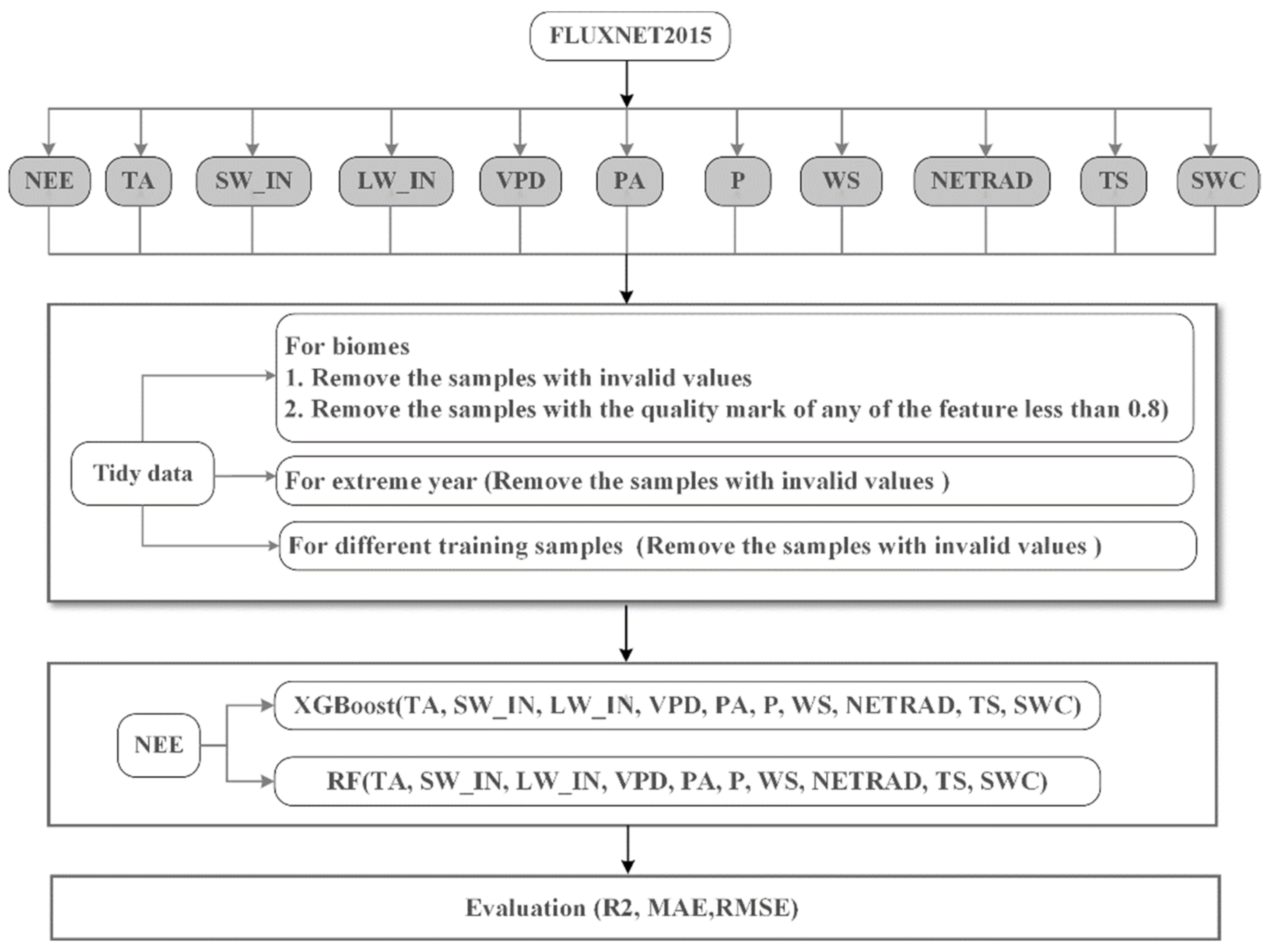
The RF and XGBoost models were implemented in this study and compared to estimate daily NEE in 10 different biomes. To achieve high simulation accuracy, the data need to be pre-processed before further analysis. We merged the subset daily data of EC sites belonging to the same biome to generate hybrid data for each biome. Because daily data were generated by aggregating half-hourly data, further sample screening was performed based on the quality mark of each feature. The quality mark ranges between 0~1, indicating the percentage of observed and good quality gap-filled half-hourly samples per day. To control the data quality of the training features, we excluded the sample when any of the feature’s quality mark was less than 0.8. After the process of data cleaning, both of the RF and XGBoost models were generated in Python (version 3.7.5) with packages including Numpy (version 1.17.3), Pandas (version 0.25.3), Scikit-learn (version 0.23.2), and Scikit-learn interface for XGBoost.
For each hybrid data of different biomes, we used the method of “train_test_split” to split it into training samples (70%) and test samples (30%) with a “random_state” value of 420. The training sample was modeled using the “randomizedSearchCV” method with 5-fold cross-validation as well as random search to obtain hyper-parameters for the model. The hyper-parameters used for the two models are listed in Table S1. Taking into account the computational efficiency, the “n_iter” parameter in the “randomizedSearchCV” method was set to 100 and 200 for RF and XGBoost, respectively. It controls the number of parameter settings that are tried in the model training. After the hyper-parameters are obtained, the best model can be established. The summary of the data processing was outlined in Figure 1.
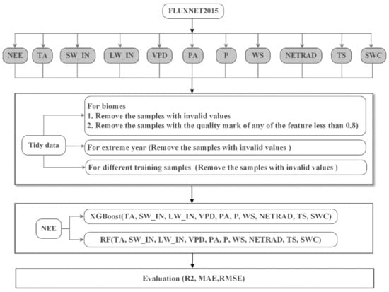
Figure 1.
Flowchart of datasets and model setup. NEE is assumed to be the nonlinear function of TA, SW_IN, LW_IN, VPD, PA, P, WS, NETRAD, TS, and SWC. (NEE: Net ecosystem exchange; TA: Air temperature; SW_IN: Shortwave radiation, incoming; LW_IN: Longwave radiation, incoming; VPD: Vapor pressure deficit; PA: Atmospheric pressure; P: Precipitation; WS: Wind speed; NETRAD: Net radiation; TS: Soil temperature at the shallowest; SWC: Soil water content at the shallowest).
2.3.2. Simulations under Extreme Climate Conditions
To analyze the applicability of the models under extreme climate conditions, we specifically evaluated the model performance in simulating NEE under extremely hot, cold, wet, or dry years. The procedures were as below. First, we selected each of the EC sites with more than 10 years of observational data. For each selected site, we calculated the respective standard deviations (SD) for the mean annual temperature (MAT) and annual total precipitation (ATP). The year is considered to be extremely cold if its MAT is less than the multi-year mean temperature by two SDs, and extremely hot if its MAT is greater than the multi-year mean temperature by two SDs. We can find the extremely dry and extremely wet years in the same way. Finally, 5 sites with extreme heat years, 7 sites with extreme cold years, 4 sites with extreme wetness years, and 3 sites with extreme dryness years were selected, details in Table S2. For each extreme situation, we selected the sites with different biomes for evaluation. If there were multiple sites with the same biome in the same extreme conditions, we randomly selected one of them. In order to maintain a balance between the number of extreme and normal samples, we selected a non-extreme year closest to the extreme year to represent the normal year. The samples of extreme year and the normal year were split into training samples (70%, merged the extreme and normal training samples for training) and validation samples (30%, representing extreme and normal samples of testing) with “random_state” value of 420, respectively. A comparison of prediction NEE for extreme and normal samples with the same modeling approach as that of biome above is shown in Section 2.3.1. Note that, in order to maintain the integrity of the data, we did not use the quality mark of each feature for sample exclusion as in Section 2.3.1.
2.3.3. Sample Size Sufficiency for Model Estimation
To quantify the effect of the number of training samples on the NEE prediction of site-level, four EC sites (US-MMS, US-Var, DE-Geb, NL-Loo) with different biomes and more than 12 years observations were selected. Two approaches were used to assess the robustness of the model prediction results with different training sample sizes. The first approach is to use the last 2 years dataset of the site as the test samples and the number of training samples is increased by the annual sample size (BAS) to build the model. The details of the annual sample size of each evaluated EC site are shown in Table S3.
Another method is to increase the number of total samples gradually by a fixed step of 100 (BFS). First, we merged the annual samples for each evaluated EC site. The total samples for each evaluation were randomly selected from the merged data, then split into 70% for training and 30% for testing. Determination (R2), root mean square error (RMSE), and mean absolute error (MAE) were used to evaluate the prediction results. The definitions of three metrics are as follows:
where is the ith observed validation sample, the predicted value of the ith validation sample, denotes the mean value of observed value y, and n is the number of validation samples. When R2 is larger and RMSE and MAE are smaller, it means that the predicted value is closer to the observed value. Evaluation of the models using these three indices can provide criteria for hyper-parameter correction and model performance comparisons.
2.4. Bernaola-Galvan Segmentation Algorithm
The Bernaola-Galvan Segmentation Algorithm (BGSA) was adopted to detect nonlinear, nonstationary sequence mutations [48]. Its principle is to divide a non-stationary time series by making the time series consist of many segments with different means, such that the difference in means between neighboring segments is maximized. Compared to traditional mutation detection methods, the BGSA showed better performance in estimating climate evolution [49,50]. In this study, we used the BGSA algorithm to detect the mutations of R2 series derived from the two machine-learning algorithms (Section 2.3.3).
2.5. Feature Analysis
Feature importance is defined as the contribution of each variable to the model, with important variables showing a greater impact on the model evaluation results. In this study, we use both impurity-based and permutation-based methods to calculate the feature importance for RF and XGBoost algorithms, respectively. RF and XGBoost are all ensemble models based on the decision tree as the base estimator, the difference between them is that each decision tree is generated in a different way. In a single decision tree, the model uses the amount of each feature split point improvement performance measure to calculate feature importance, called the impurity-based importance measure. It is used to describe how useful each feature is in constructing the decision tree in the model. However, when the model is overfitting, some features that have less predictive effect may get high importance. The permutation importance is the decrease in a model score when a single feature value is not available, which is complementary to the impurity-based im-portance. In this study, the impurity-based predictive importance scores of features were obtained from the attribute of “feature_importances_” of the best trained RF or XGBoost models generated during the modeling development. The feature importance of the two models and different biomes will be output by the above processes. The permutation-based predictive importance scores used the method of “permutation_importance” to evaluate the training samples with a “n_repeats” value of 10.
3. Results
3.1. Biome-Level Model Performance
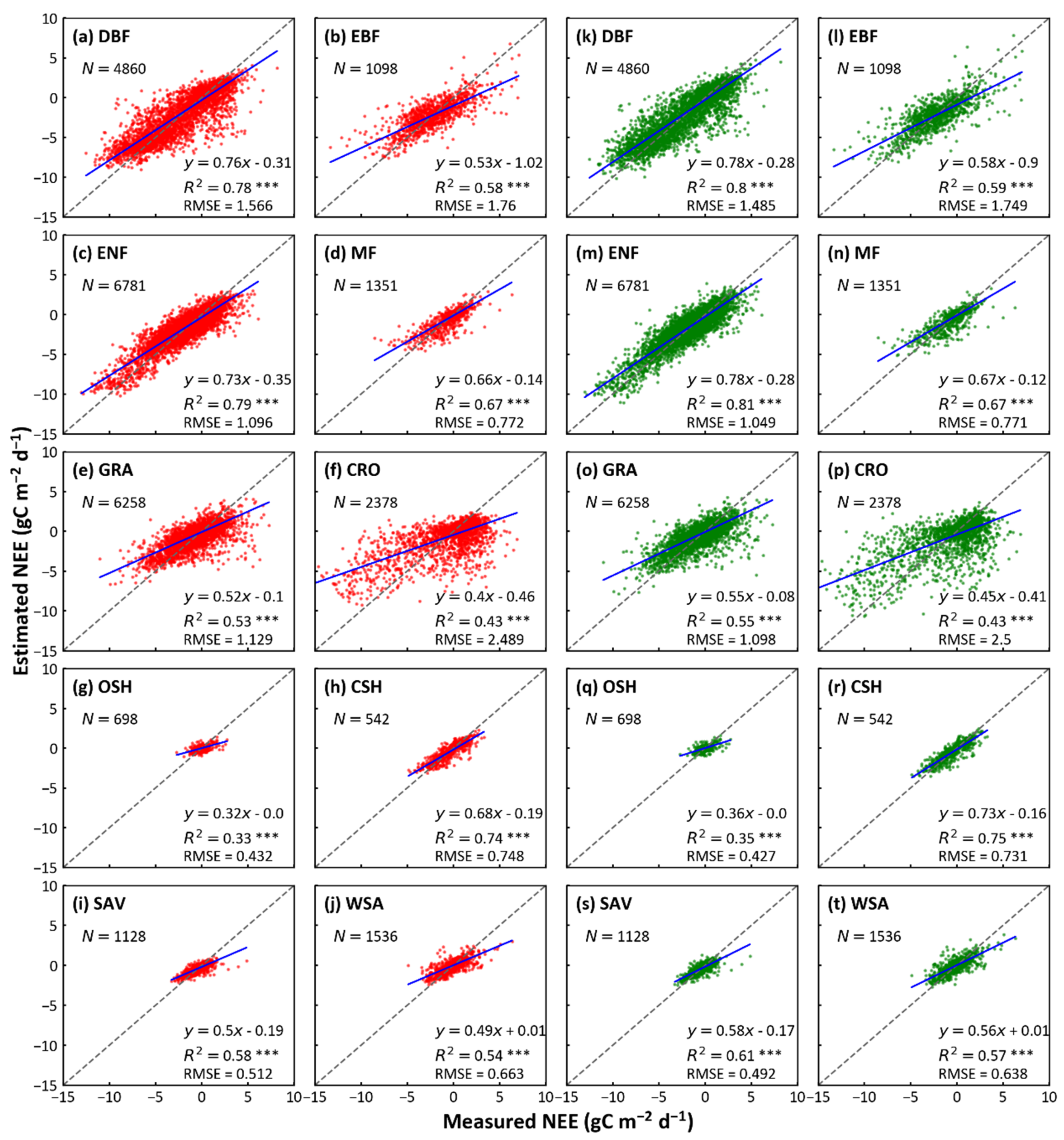
The RF and XGBoost algorithms did reasonably well in simulating NEE at the biome-level (Figure 2). Among eight biomes (DBF, EBF, ENF, GRA, OSH, CSH, SAV, and WSA), XGBoost predicted slightly better than RF, with larger R2 and smaller RMSE; for the other two biomes (MF and CRO), the predictions of the two models have the same R2 and RMSE. For the XGBoost, ENF (R2 = 0.81 and RMSE = 0.77 g C m−2d−1) has the highest R2 and OSH shows the smallest R2 (R2 = 0.35 and RMSE = 0.43 g C m−2d−1). In summary, the forest ecosystems (DBF, EBF, ENF, and MF) have the best predictions (R2 between 0.59 to 0.81), followed by savanna (contain SAV and WSA; R2 between 0.57 to 0.61), grassland (R2 = 0.55), and cropland (R2 = 0.43). The predictions of different types of shrublands (OSH and CSH) showed a large inconsistency, with the R2 of CSH (R2 = 0.75) being much higher than that of OSH (R2 = 0.35). From the fitted lines, the predicted values of both models were smaller than the observed values, in all biomes. Although the prediction of XGBoost is as similar as that of RF, XGBoost is slightly better in modeling efficiencies. The training durations for RF and XGBoost with different biomes of training samples are shown in Table 3. For different biomes, the training durations of different models increase reasonably with the number of training samples. The computational efficiency of XGBoost is 6~62 times higher than that of RF, and their difference increases as the number of samples increases.
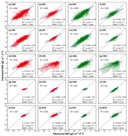
Figure 2.
Comparison of predicted and actual values using RF and XGBoost models in each biome. The x-axis represents actual values of NEE by eddy-covariance and y-axis denotes the predicted values by the two models above. The red and green scatters indicate the prediction of RF and XGBoost for each biome, respectively. The dash line represents the equality of predicted and actual values. R2 refers to the determination, RMSE refers to root mean square error, N refers to the number of test data points. * p-value ≤ 0.05, ** p-value ≤ 0.01, and *** p-value ≤ 0.001. (DBF, deciduous broadleaf forest; EBF, evergreen broadleaf forest; ENF, was evergreen needleleaf forest; MF, mixed forest; GRA, grassland; CRO, cropland; OSH, open shrublands; CSH, closed shrublands; SAV, savannas; WSA, woody savannas).

Table 3.
Training duration for different biomes and models.
3.2. Environmental Conditions
The feature rankings obtained by impurity-based and permutation-based were generally consistent across biomes (Figure 3 and Figure S1). For the impurity-based result (Figure 3), there were two biomes in the two models with the top three consistent importance of variables (DBF, in order of soil temperature (TS), net radiation(NETRAD), and atmospheric pressure (PA); WSA, in order of PA, NETRAD, and incident longwave radiation (LW_IN)), and six biomes with two identical variables in the top three of variable importance (EBF with PA and LW_IN; ENF with NETRAD and wind speed (WS); MF with NETRAD and TS; GRA with NETRAD and TS; CRO with NETRAD and vapor pressure deficit (VPD); CSH with NETRAD and LW_IN; SAV with WS and VPD; and WSA with PA and LW_IN). The biome of OSH has one identical variable in the top three of variable importance soil water content (SWC). Among all the biomes, the number of occurrences for variables in the top three variable importance was: eight occurrences of NETRAD; five occurrences of PA; three occurrences of LW_IN, SW_IN, and TS for RF model; and seven occurrences of NETRAD, five occurrences of PA, and two occurrences of LW_IN and SWC for XGBoost model. The variables with the highest number of occurrences in the last three of variable importance was precipitation (P) (nine occurrences), WS (five occurrences), LW_IN (four occurrences) for RF model; and P (eight occurrences), WS (six occurrences), LW_IN (four occurrences) for XGBoost model. In general, NETRAD, PA, and TS are the most important variables, P and WS are the least important variables in each biome for both two models.
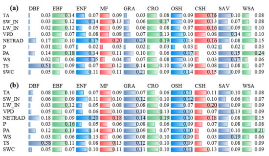
Figure 3.
Impurity-based importance of variables in RF (a) and XGBoost (b) models to NEE by biomes (NEE: Net ecosystem exchange; TA: Air temperature; SW_IN: Shortwave radiation, incoming; LW_IN: Longwave radiation, incoming; VPD: Vapor pressure deficit; PA: Atmospheric pressure; P: Precipitation; WS: Wind speed; NETRAD: Net radiation; TS: Soil temperature at the shallowest; SWC: Soil water content at the shallowest).
Similar results appear in the permutation-based method (Figure S1). Among all the biomes, the number of occurrences for variables in the top three variable importance was: NETRAD (eight occurrences), PA (seven occurrences), SWC (four occurrences) for RF model; NETRAD (eight occurrences), PA (five occurrences), and SWC (four occurrences) for XGBoost model. The variables with the highest number of occurrences in the last three of variable importance were P (ten occurrences), WS (five occurrences), LW_IN (four occurrences) for RF model; and P (ten occurrences), WS (six occurrences), LW_IN (five occurrences) for XGBoost model. Note that because of the different calculation principles, the values reported in Figure 3 are not directly comparable with that in Figure S1.
The two feature importance methods disagree on the performance of LW_IN. For both RF and XGBoost algorithms, permutation-based method showed that LW_IN was the less important variable. However, the impurity-based method showed LW_IN appears at two extremes under different biomes. For EBF, CSH, and WSA, it is an important variable (top three of variable importance), while for DBF, ENF, and OSH, it is an insignificant variable (last three of variable importance).
3.3. Model Performance in Simulating NEE under Extreme Climate Conditions
Both RF and XGBoost models captured the difference of the NEE predictions under normal and extreme climate conditions, with similar R2 and RMSE. However, dominant variables varied under different extreme conditions and in different biomes. In the following, we will use the prediction results of XGBoost as an example. Extreme cold conditions had little impacts on forest biomes (DBF, R2 = 0.93 for normal and R2 = 0.86 for extreme; ENF, R2 = 0.90 for normal and R2 = 0.87 for extreme; EBF, R2 = 0.21 for normal and R2 = 0.19 for extreme), and had a slightly greater effect on SAV (R2 = 0.53 for normal and R2 = 0.44 for extreme). Extreme heat conditions reduced the evaluation results of the four biomes, MF (R2 = 0.81 for normal and R2 = 0.76 for extreme), DBF (R2 = 0.87 for normal and R2 = 0.78 for extreme), ENF (R2 = 0.59 for normal and R2 = 0.51 for extreme), and GRA (R2 = 0.78 for normal and R2 = 0.66 for extreme) with different degrees. The negative effect of extreme wetness on CRO (R2 = 0.84 for normal and R2 = 0.64 for extreme) was significant, but showed litter effects or even positive effects on forest biomes, MF (R2 = 0.83 for normal and R2 = 0.82 for extreme), ENF (R2 = 0.90 for normal and R2 = 0.92 for extreme), and DBF (R2 = 0.86 for normal and R2 = 0.83 for extreme). In the extreme dryness conditions, DBF (R2 = 0.85for normal and R2 = 0.90 for extreme) was not affected, but SAV (R2 = 0.73 for normal and R2 = 0.43 for extreme) and GRA were evaluated with significant decreases compared to the normal condition, especially the effect for GRA was considerable (R2 = 0.54 for normal and R2 = 0.14 for extreme) (Table 4).

Table 4.
Comparative analysis of NEE predicted by the RF and XGBoost in extreme climate conditions, (a–d) denote extreme cold, extreme heat, extreme wetness, and extreme dryness, respectively. Normal refers to the evaluation of the non-extreme samples. The screening method for each extreme site and year is described in Section 2.3.2.
3.4. Model Performance in Simulating NEE under Extreme Climate Conditions
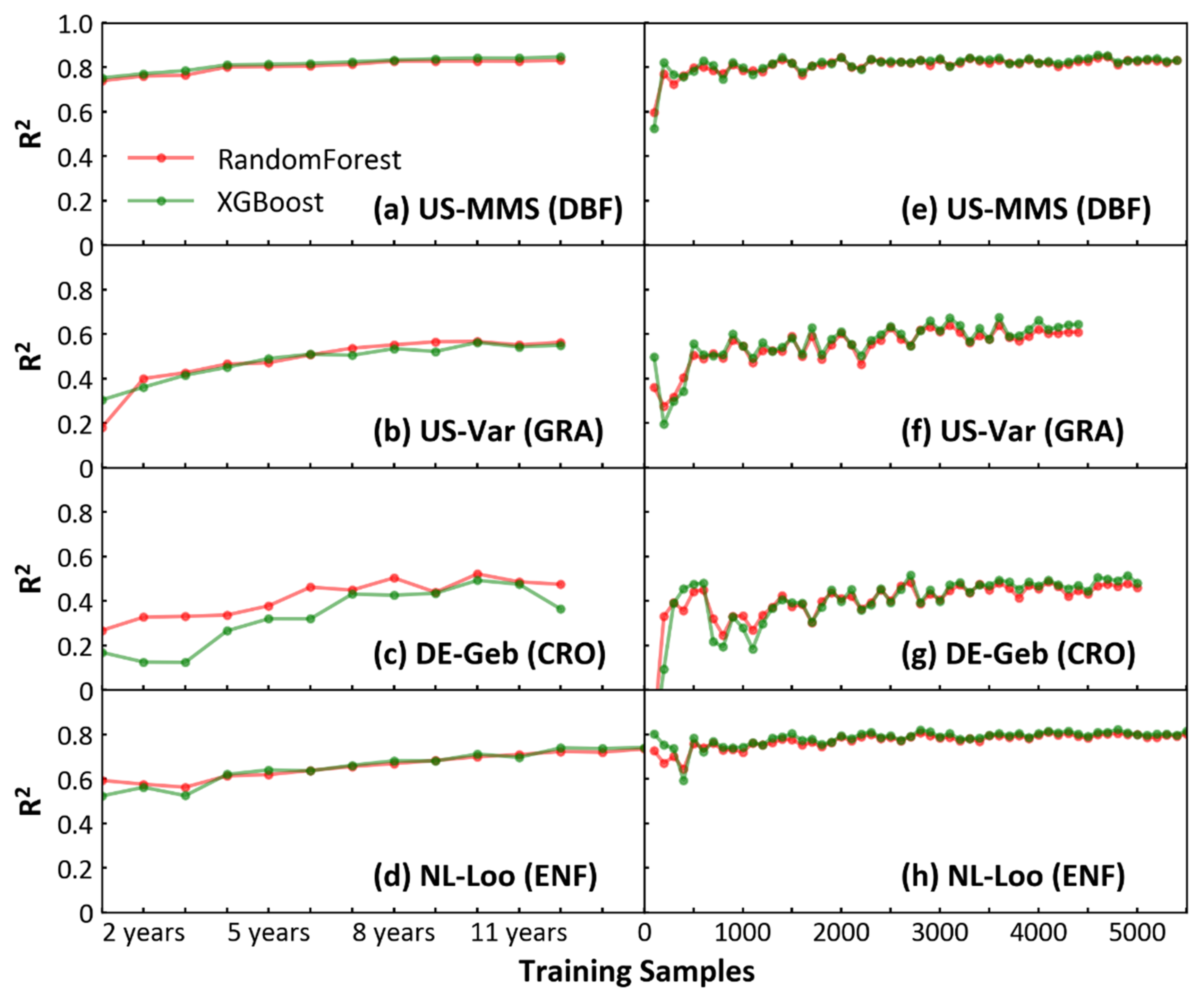
Machine learning models appear to be highly dependent on the training samples. Increasing model training samples benefits model prediction for the same quality of data [37]. Both RF and XGBoost algorithms are sensitive to the number of training samples (NTS) when simulating the NEE of different biomes at site-level. The prediction results of two models were similar according to BAS (Figure 4a–d) or BFS (Figure 4e–h) method. With the BAS method, the result of XGBoost showed that the R2 of the prediction for the four sites increased with the NTS and reached a stable state when the NTS reached about 8 years of daily samples (Figure 4a–d). With the BFS method, when the assessment curve reached final stability, the R2 assessed by each site (US-MMS, R2 = 0.83; US-Var, R2 = 0.64; DE-Geb, R2 = 0.48; NL-Loo, R2 = 0.79) was generally consistent with the evaluation result of the respective biome to which they belong in Figure 2. In Figure 4e–h, although the prediction of each site eventually reached a steady state with the maximum R2 as the NTS increased, the R2 curves varied among biomes. For the forest biome (Figure 4e,h), R2 reached a steady-state faster with the increase of samples and low fluctuation before the steady state. For GRA and CRO (Figure 4f,g), in contrast to the forest biome, R2 reached a steady-state more slowly and large fluctuation before the steady state.
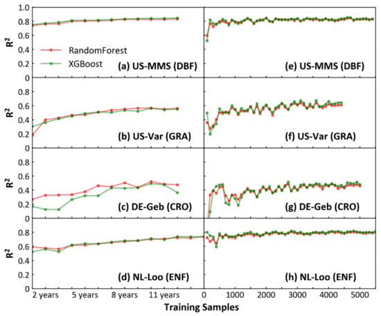
Figure 4.
(a–d) Effect of increasing the training sample on the prediction results (take four sites as examples). Increasing training samples in terms of annual sample size (x axis) and the determination (R2) from each test sample and predicted values (y axis). (e–h) Increase the total samples (70% of which are training samples and 30% are test samples) in steps of 100 (x axis), and the determination (R2) as in (a–d).
3.5. Quantitative Analysis of Sample Size in Reaching Feasible Model Performance
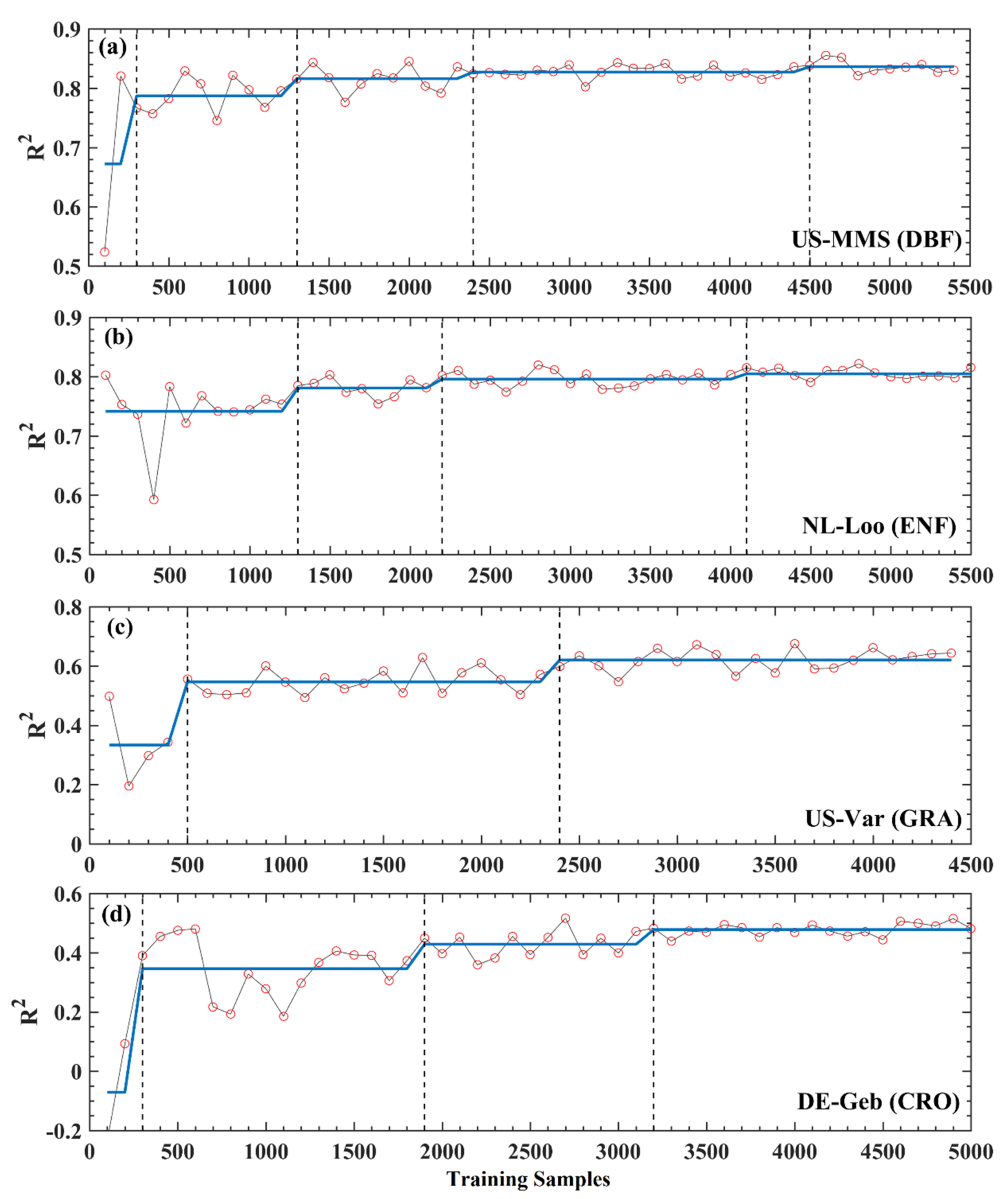
To quantitatively determine the effects of the sample number on the model prediction, the BGSA algorithm was used to test the R2 curves of XGBoost in Figure 4e–h for mutation. In Figure 5, the mutation points ranged from two to four for different sites (US-MMS, DBF, with 4; NL-Loo, ENF, with 3; US-Var, GRA, with 2; and DE-Geb, CRO, with 3). Except for the NL-Loo site, the first mutation position of the other three sites is less than 500. At the left of the first mutation, each curve of R2 fluctuates dramatically and a distinct trough appears. This is likely because when the total sample size is less than 500, then the NTS is less than 350 (approximately one complete observation year), so the NTS is not representative enough. Since both US-MMS (DBF) and NL-Loo (ENF) sites (Figure 5a,b) belong to the forest biome, their mutations are basically the same, at 1300, 2200–2400, and 4100–4500, respectively. The R2 values increase after each mutation. The x-axis in Figure 5 refers to the total number of samples (70% of which are training samples and 30% are test samples), so the NTS corresponding to each mutation is 910, 1540–1680 (the median is about 1600), and 2870–3150 (the median is about 3000). This means for DBF and ENF sites, the training sample number of 910 (approximately 2.5 years daily samples, named YDS hereafter) can stabilize the model, and 3000 (approximately 8.2 YDS) can lead the model to reach the best performance. Compared with the above two sites, US-Var (GRA) and DE-Geb (CRO) sites (Figure 5c,d) reached the stability mutation at delayed positions between 1900 to 2400 (the median is equal to 2150) and the last mutation at an earlier position between 2400 to 3200 (the median is equal to 2800); correspondingly, the NTS are 1505 (approximately 4.1 YDS) and 1960 (approximately 5.4 YDS), respectively. The same trend was observed in the RF analysis for both four sites, detailed in Figure S3.
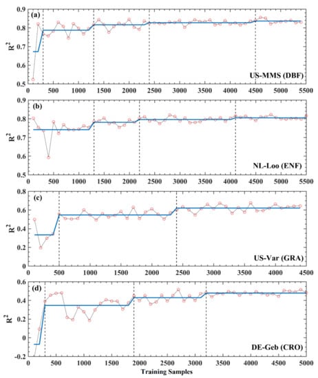
Figure 5.
Mutation detections for the evaluation results of XGBoost in Figure 4e–h by the BG segmentation algorithm. The black vertical dash lines represent mutation points.
4. Discussion
4.1. Quantitative Analysis of Sample Size in Reaching Feasible Model Performance
The studies compared two algorithms in simulating NEE (Table 5). Predictions of XGBoost for forest biome in this study were generally better than SVR [33]; for XGBoost, the evaluation metrics (R2) of DBF, EBF, ENF, and MF were 0.78, 0.58, 0.79, and 0.67 respectively, and for SVR they were 0.78, 0.59, 0.29, and 0.37 respectively; GRA also had a similar result, the R2 of XGBoost and SVR were 0.55 and 0.37, respectively; but SVR had a better prediction for CRO, with a higher R2 of 0.60 compared to 0.43 of XGBoost. For the forest biome (DBF, ENF, MF), XGBoost (with R2 between 0.59–0.81) prediction was similar to the results of the best prediction in adaptive neuro-fuzzy inference system (ANFIS), extreme learning machine (ELM), artificial neural network (ANN), and support vector machine (SVM) model, with R2 between 0.59 and 0.80 [39]. Note that the XGBoost training samples are the hybrid data from multiple EC sites, while the predictions of Dou et al. [39] are for a single EC site. Similar prediction results were obtained for the bamboo forest sample sites using the RF method (R2 = 0.68) [50]. Jung et al. [36] used the MTE model to obtain predictions of NEE with R2 = 0.49 from multiple EC sites (no biome distinction) around the world.

Table 5.
Synthesis of NEE predicted by data-drive methods. List of acronyms: Cor, correlation coefficient; R2, determination; MAE, mean absolute error; RMSE, root mean square error; DBF, deciduous broadleaf forest; EBF, evergreen broadleaf forest; ENF, evergreen needleleaf forest; MF, mixed forest; GRA, grassland; CRO, cropland; OSH, open shrublands; CSH, closed shrublands; SAV, savannas; WSA, woody savannas; TUN, tundra; GBR, gradient boosting regression; SVM, support vector machine; SGD, stochastic gradient descent; BR, Bayesian ridge; RF, Random Forest; Model tree ensembles, MTE; SVR, support vector regression; SVR, support vector regression; ANFIS, adaptive neuro-fuzzy inference system; ELM, extreme learning machine; ANN, artificial neural network; SVM, support vector machine; XGBoost, Extreme Gradient Boosting.
Some predictions using the gradient boosting regression (GBR) method are better than using XGBoost to predict an EC site of ENF (with R2 = 0.90 for GBR and R2 = 0.81 for XGBoost) [37]. This likely arises for two reasons. First, the GBR method used a single site data for training. Due to the differences in climate and ecological environments of different EC sites, the prediction of a single site will be better than the hybrid data of multiple sites. We evaluated the same EC site and time period as Cai et al. [37] did with XGBoost method. The evaluation results showed a slight improvement over biome-level simulation of ENF, which the site belongs to (with R2 = 0.81 and RMSE = 1.049 g C m−2d−1 for ENF biome and R2 = 0.824 and RMSE = 0.802 g C m−2d−1 for site-level). Second, the impact of extreme components (maximums and minimums) of the variables on the model was considered when training the GBR model. Therefore, we believe that under the same conditions the prediction of NEE by XGBoost generally meets expectations and is better than most other popular ML methods. It should be noted that all previous studies use multi-source data for model training, such as remote sensing data of vegetation, meteorology data etc., while we only use the meteorology data, which is the least number of data sources and environmental variables. It shows that single source and fewer environmental variables still have a good prediction effect on NEE. Similar results were reported for the prediction of NEE using meteorological data alone comparing the combination of meteorological and remote sensing data for model training [38].
4.2. Environmental Controls as Estimated by Two ML Algorithms
It has been shown that radiation, air and soil temperature, relative humidity, vapor pressure deficit, and wind speed were the main factors affecting NEE [51]. In this study, a combination of both impurity-based and permutation-based methods indicated that NETRAD, PA, SWC, and TS were the most important variables, but P and WS were the least important variables when considering all biomes together. We found that other machine learning methods also have the same results [37,52]. This is because traditional statistical methods are based on the classical hypothetico-deductive approach, while ML methods build relationships directly from the data and fit highly non-linear relations between input and output data. For example, although precipitation is an important resource to ensure plant physiological activities, the effect of precipitation on carbon fluxes is generally reflected on an interannual scale [53]. Since the training data we used are based on daily values, and the daily precipitation is not directly responsible for the daily NEE change. This may be the main reason that XGBoost shows inconsistency with traditional statistical methods. In summary, the feature importance from the ML models serves two purposes: one is to provide further insight into the underlying process of NEE generation, and the other is to help in the pre-modeling phase for feature engineering optimization, with the latter being probably more useful. The two methods corroborated each other and showed better consistency, this increased our confidence concerning the feature importance result. It also indicated that the modeling did not have obvious overfitting in this study.
We also took mixed forest samples as an example to build the model for different seasons and output each of the feature importance. For the result as described in Figure S2, the results of both RF and XGBoost had similar distributions across seasons and the year. Seasonal variation of the feature importance does exist. The value of shortwave radiation and NETRAD was significantly higher in summer and autumn than in other seasons; while TS and SWC had relatively low values in autumn. This suggests that a more proper split of the samples, such as by season, may obtain more detailed information on the feature importance and improve the performance of the model.
4.3. Effects of Extreme Climatic Conditions on NEE Prediction at Biome Level
Extreme climatic conditions can affect the growth and development of vegetation by altering its physiological processes [54]. This is also reflected in the data-based ML method as the input variables under extreme weather can affect the model driving. However, this influence needs to be related with different extreme conditions as well as different biomes. This corresponds to the environmental conditions required for different biomes. The forest and SAV sites used in the study are mostly located at middle and high latitudes, and they are adaptable to low temperatures, so extreme cold has little effect on their prediction results. Both extreme heat and extreme dryness have effects on vegetation growth in different biomes, but the effects of extreme dryness are more pronounced. Extreme wetness has little or no effect for forest, but does not apply to CRO.
4.4. Effects of Extreme Climatic Conditions on NEE Prediction at Biome Level
Both RF and XGBoost methods had good prediction accuracy for NEE, which shows that the tree-based ML methods have an advantage in CO2 flux prediction. In general, the XGBoost model has better prediction results than RF in all biomes with higher R2 and lower RMSE; XGBoost offers more efficient computation than RF. For XGBoost, the number of training samples and training duration show a highly linear relationship (y = 0.0004x − 0.226, R2 = 0.998, p < 0.0001; x refers to the number of training samples, and y refers to the training duration which unit is minute), while RF shows a significant exponential relationship (y = 10−6x1.979, R2 = 0.992, p < 0.0001) (Figure S4). That means, XGBoost can get better performance than RF with less computational cost. Moreover, the XGBoost algorithm is complex with many hyper-parameters, and the prediction accuracy of XGBoost may still be improved after an optimized hyper-parameter. However, due to the inability of the tree-based ML methods in extrapolation, the model predicted that NEE is smaller than the observational results. In conclusion, the XGBoost method shows better prediction accuracy and computational efficiency in predicting NEE.
5. Conclusions
In this study, we applied two machine learning algorithms, RF and XGBoost, to simulate NEE in major biomes across the globe. We found that the XGBoost has a better model performance than the RF with a 6–62 times higher computational efficiency. The robustness of the two methods was also tested for different extreme climate conditions and the different numbers of training samples. Both XGBoost and RF reflect the difference of prediction between extreme condition samples and normal samples well. The training sample size impact on model performance varied by biome. Biomes with better model performance (DBF and ENF) were easier to achieve the first stability with a smaller NTS and continued to optimize with increasing NTS, while the opposite applied to GRA and CRO biomes. In general, a minimum of 8 years of daily training dataset will lead to feasible model prediction for various biomes.
The variables used for the model training include 10 meteorological variables, which is slightly less than other studies. Both RF and XGBoost algorithms produced feasible results, which indicates that the variables other than those used in this study have slight contribution to the NEE prediction. Given the strengths of XGBoost, it could have good implications on upscaling NEE prediction from the site to a regional area in the future, e.g., based on grouping of samples under normal and extreme climate conditions. It also provides the potential application for estimating NEE from satellite-derived data, which should be very helpful for regional and global scale.
Supplementary Materials
The following are available online at https://www.mdpi.com/article/10.3390/rs13122242/s1. Table S1 Hyper-parameters used for the models and the initial settings with randomized SearchCV method, Table S2 List of sites with extreme conditions. Acronyms: MAT, mean annual temperature; MMT, multi-year mean temperature; AP, annual precipitation; MMP, multi-year mean precipitation; SD, standard deviations of temperature or precipitation for the listed sites; DBF, deciduous broadleaf forest; EBF, evergreen broadleaf forest; ENF, was evergreen needleleaf forest; MF, mixed forest; GRA, grassland; CRO, cropland; SAV, savannas, Table S3 Number of training and testing samples used for quantitative analysis of model performance, Figure S1 Permutation-based importance of variables in predicting NEE by (a) RF and (b) XGBoost (b) at biome level (NEE: Net ecosystem exchange; TA: Air temperature; SW_IN: Shortwave radiation, incoming; LW_IN: Longwave radiation, incoming; VPD: Vapor pressure deficit; PA: Atmospheric pressure; P: Precipitation; WS: Wind speed; NETRAD: Net radiation; TS: Soil temperature in the top soils; SWC: Soil water content in the top soils (0–5 cm), Figure S2 Feature importance of variable in predicting NEE by (a) Random Forest and (b) XGBoost methods with the mixed forest as an example. The colors of each grid reflect the value of feature importance, darker color indicates more important, Figure S3 Mutation detection performed on the evaluation results of Random Forest corresponding to the Figure 4e–h by the BG segmentation algorithm. The x axis and y axis values are the same as in Figure 4e–h. The black vertical dash lines represent mutation points, Figure S4 Correlation between training samples and training duration for (a) RF and (b) XGBoost.
Author Contributions
Conceptualization, X.X.; methodology, J.L., F.Y., and X.S.; software, J.L.; validation, J.L. and Y.Z.; resources, C.S. and Y.G.; data curation, J.L.; writing—original-draft preparation, J.L.; result interpretation: all; writing—review and editing, X.X., F.Y., N.W., Y.Z., L.Z., X.Z., Z.G., Y.S. and J.Z.; visualization, J.L.; supervision, X.X.; project administration, F.Y. and X.X.; funding acquisition, C.S. All authors have read and agreed to the published version of the manuscript.
Funding
This study was partially supported by the National Key R&D Program (2016YFA0602303), the National Natural Science Foundation (No. 41730643, 41975150, 41701198) of China, Liaoning Provincial Natural Science Foundation (2020-MS-027), Ecology Innovation Team(2020CXTD02) in Minzu University of China, and Northeast Institute of Geography and Agroecology, Chinese Academy of Sciences. X.X. and F.Y. are grateful for the financial and facility support from San Diego State University.
Institutional Review Board Statement
Not applicable.
Informed Consent Statement
Not applicable.
Data Availability Statement
The codes used in this study are available upon request from the authors.
Acknowledgments
This work used eddy covariance data from the FLUXNET community (https://fluxnet.org/ accessed on 18 April 2021). Thanks to the software provider of Scikit-learn package (https://github.com/scikit-learn/scikit-learn accessed on 18 April 2021) and XGBoost package (https://github.com/dmlc/xgboost accessed on 18 April 2021). We would like to thank these organizations for providing great data-sharing and soft platforms. Their contributions made this work possible. We would like to thank each individual explicitly here but cannot do so due to limited space.
Conflicts of Interest
The authors declare no conflict of interest.
References
- Post, W.M.; Peng, T.-H.; Emanuel, W.R.; King, A.W.; Dale, V.H.; DeAngelis, D.L. The global carbon cycle. Am. Sci. 1990, 78, 310–326. [Google Scholar]
- Friend, A.D.; Arneth, A.; Kiang, N.Y.; Lomas, M.; Ogee, J.; Rödenbeck, C.; Running, S.W.; Santaren, J.D.; Sitch, S.; Viovy, N. FLUXNET and modelling the global carbon cycle. Glob. Chang. Biol. 2007, 13, 610–633. [Google Scholar] [CrossRef]
- Isson, T.T.; Planavsky, N.J.; Coogan, L.A.; Stewart, E.M.; Ague, J.J.; Bolton, E.W.; Zhang, S.; McKenzie, N.R.; Kump, L.R. Evolution of the global carbon cycle and climate regulation on Earth. Glob. Biogeochem. Cycles 2020, 34, e2018GB006061. [Google Scholar] [CrossRef]
- Chapin, F.S.; Woodwell, G.M.; Randerson, J.T.; Rastetter, E.B.; Lovett, G.M.; Baldocchi, D.D.; Clark, D.A.; Harmon, M.E.; Schimel, D.S.; Valentini, R.; et al. Reconciling Carbon-cycle Concepts, Terminology, and Methods. Ecosystems 2006, 9, 1041–1050. [Google Scholar] [CrossRef]
- Baldocchi, D.D. Assessing the eddy covariance technique for evaluating carbon dioxide exchange rates of ecosystems: Past, present and future. Glob. Chang. Biol. 2003, 9, 479–492. [Google Scholar] [CrossRef]
- Pastorello, G.; Trotta, C.; Canfora, E.; Chu, H.; Christianson, D.; Cheah, Y.W.; Poindexter, C.; Chen, J.; Elbashandy, A.; Humphrey, M.; et al. The FLUXNET2015 dataset and the ONEFlux processing pipeline for eddy covariance data. Sci. Data 2020, 7, 225. [Google Scholar] [CrossRef] [PubMed]
- Baldocchi, D.D.; Hincks, B.B.; Meyers, T.P. Measuring Biosphere-Atmosphere Exchanges of Biologically Related Gases with Micrometeorological Methods. Ecology 1988, 69, 1331–1340. [Google Scholar] [CrossRef]
- Baldocchi, D.; Falge, E.; Gu, L.H.; Olson, R.; Hollinger, D.; Running, S.; Anthoni, P.; Bernhofer, C.; Davis, K.; Evans, R.; et al. FLUXNET: A new tool to study the temporal and spatial variability of ecosystem-scale carbon dioxide, water vapor, and energy flux densities. Bull. Am. Meteorol. Soc. 2001, 82, 2415–2434. [Google Scholar] [CrossRef]
- Sitch, S.; Smith, B.; Prentice, I.C.; Arneth, A.; Bondeau, A.; Cramer, W.; Kaplan, J.O.; Levis, S.; Lucht, W.; Sykes, M.T.; et al. Evaluation of ecosystem dynamics, plant geography and terrestrial carbon cycling in the LPJ dynamic global vegetation model. Glob. Chang. Biol. 2003, 9, 161–185. [Google Scholar] [CrossRef]
- Krinner, G.; Viovy, N.; de Noblet-Ducoudre, N.; Ogee, J.; Polcher, J.; Friedlingstein, P.; Ciais, P.; Sitch, S.; Prentice, I.C. A dynamic global vegetation model for studies of the coupled atmosphere-biosphere system. Glob. Biogeochem. Cycles 2005, 19. [Google Scholar] [CrossRef]
- Lawrence, D.M.; Oleson, K.W.; Flanner, M.G.; Thornton, P.E.; Swenson, S.C.; Lawrence, P.J.; Zeng, X.B.; Yang, Z.L.; Levis, S.; Sakaguchi, K.; et al. Parameterization Improvements and Functional and Structural Advances in Version 4 of the Community Land Model. J. Adv. Model. Earth Syst. 2011, 3. [Google Scholar] [CrossRef]
- Xu, X.; Elias, D.A.; Graham, D.E.; Phelps, T.J.; Carroll, S.L.; Wullschleger, S.D.; Thornton, P.E. A microbial functional group-based module for simulating methane production and consumption: Application to an incubated permafrost soil. J. Geophys. Res. Biogeosci. 2015, 120, 1315–1333. [Google Scholar] [CrossRef]
- Wang, Y.; Yuan, F.; Yuan, F.; Gu, B.; Hahn, M.S.; Torn, M.S.; Ricciuto, D.M.; Kumar, J.; He, L.; Zona, D.; et al. Mechanistic Modeling of Microtopographic Impacts on CO2 and CH4 Fluxes in an Alaskan Tundra Ecosystem Using the CLM-Microbe Model. J. Adv. Model. Earth Syst. 2019, 11, 4288–4304. [Google Scholar] [CrossRef]
- Jung, M.; Schwalm, C.; Migliavacca, M.; Walther, S.; Reichstein, M. Scaling carbon fluxes from eddy covariance sites to globe: Synthesis and evaluation of the FLUXCOM approach. Biogeosciences 2020, 17, 1343–1365. [Google Scholar] [CrossRef]
- Zeng, J.; Matsunaga, T.; Tan, Z.H.; Saigusa, N.; Shirai, T.; Tang, Y.; Peng, S.; Fukuda, Y. Global terrestrial carbon fluxes of 1999–2019 estimated by upscaling eddy covariance data with a random forest. Sci. Data 2020, 7, 313. [Google Scholar] [CrossRef] [PubMed]
- Tian, H.; Xu, X.; Lu, C.; Liu, M.; Ren, W.; Chen, G.; Melillo, J.; Liu, J. Net exchanges of CO2, CH4, and N2O between China’s terrestrial ecosystems and the atmosphere and their contributions to global climate warming. J. Geophys. Res. Biogeosci. 2011, 116. [Google Scholar] [CrossRef]
- Tian, H.; Chen, G.; Zhang, C.; Liu, M.; Sun, G.; Chappelka, A.; Ren, W.; Xu, X.; Lu, C.; Pan, S.; et al. Century-Scale Responses of Ecosystem Carbon Storage and Flux to Multiple Environmental Changes in the Southern United States. Ecosystems 2012, 15, 674–694. [Google Scholar] [CrossRef]
- Song, X.; Tian, H.Q.; Xu, X.F.; Hui, D.F.; Chen, G.S.; Sommers, G.; Marzen, L.; Liu, M.L. Projecting terrestrial carbon sequestration of the southeastern United States in the 21st century. Ecosphere 2013, 4, 18. [Google Scholar] [CrossRef]
- Li, X.; Hu, X.-M.; Cai, C.; Jia, Q.; Zhang, Y.; Liu, J.; Xue, M.; Xu, J.; Wen, R.; Crowell, S.M.R. Terrestrial CO2 Fluxes, Concentrations, Sources and Budget in Northeast China: Observational and Modeling Studies. J. Geophys. Res. Atmos. 2020, 125. [Google Scholar] [CrossRef]
- Sefrin, O.; Riese, F.M.; Keller, S. Deep Learning for Land Cover Change Detection. Remote Sens. 2021, 13, 78. [Google Scholar] [CrossRef]
- Kianian, B.; Liu, Y.; Chang, H.H. Imputing Satellite-Derived Aerosol Optical Depth Using a Multi-Resolution Spatial Model and Random Forest for PM2.5 Prediction. Remote Sens. 2021, 13, 126. [Google Scholar] [CrossRef]
- Xiao, J.; Ollinger, S.V.; Frolking, S.; Hurtt, G.C.; Hollinger, D.Y.; Davis, K.J.; Pan, Y.; Zhang, X.; Deng, F.; Chen, J.; et al. Data-driven diagnostics of terrestrial carbon dynamics over North America. Agric. For. Meteorol. 2014, 197, 142–157. [Google Scholar] [CrossRef]
- Zhang, J.X.; Liu, K.; Wang, M. Downscaling Groundwater Storage Data in China to a 1-km Resolution Using Machine Learning Methods. Remote Sens. 2021, 13, 523. [Google Scholar] [CrossRef]
- Kim, Y.; Johnson, M.S.; Knox, S.H.; Black, T.A.; Dalmagro, H.J.; Kang, M.; Kim, J.; Baldocchi, D. Gap-filling approaches for eddy covariance methane fluxes: A comparison of three machine learning algorithms and a traditional method with principal component analysis. Glob. Chang. Biol. 2020, 26, 1499–1518. [Google Scholar] [CrossRef]
- Jordan, M.I.; Mitchell, T.M. Machine learning: Trends, perspectives, and prospects. Science 2015, 349, 255. [Google Scholar] [CrossRef]
- Arel, I.; Rose, D.C.; Karnowski, T.P. Deep Machine Learning-A New Frontier in Artificial Intelligence Research [Research Frontier]. IEEE Comput. Intell. Mag. 2010, 5, 13–18. [Google Scholar] [CrossRef]
- Feng, Q.Y.; Vasile, R.; Segond, M.; Gozolchiani, A.; Wang, Y.; Abel, M.; Havlin, S.; Bunde, A.; Dijkstra, H.A. ClimateLearn: A machine-learning approach for climate prediction using network measures. Geosci. Model. Dev. Discuss. 2016, 2016, 1–18. [Google Scholar] [CrossRef]
- Quade, M.; Gout, J.; Abel, M. Glyph: Symbolic Regression Tools. J. Open Res. Softw. 2019, 7. [Google Scholar] [CrossRef]
- Van Wijk, M.T.; Bouten, W. Water and carbon fluxes above European coniferous forests modelled with artificial neural networks. Ecol. Model. 1999, 120, 181–197. [Google Scholar] [CrossRef]
- Melesse, A.M.; Hanley, R.S. Artificial neural network application for multi-ecosystem carbon flux simulation. Ecol. Model. 2005, 189, 305–314. [Google Scholar] [CrossRef]
- He, H.; Yu, G.; Zhang, L.; Sun, X.; Su, W. Simulating CO2 flux of three different ecosystems in ChinaFLUX based on artificial neural networks. Sci. China Ser. D Earth Sci. 2006, 49, 252–261. [Google Scholar] [CrossRef]
- Kondo, M.; Ichii, K.; Takagi, H.; Sasakawa, M. Comparison of the data-driven top-down and bottom-up global terrestrial CO2exchanges: GOSAT CO2inversion and empirical eddy flux upscaling. J. Geophys. Res. Biogeosci. 2015, 120, 1226–1245. [Google Scholar] [CrossRef]
- Ichii, K.; Ueyama, M.; Kondo, M.; Saigusa, N.; Kim, J.; Carmelita Alberto, M.; Ardoe, J.; Euskirchen, E.S.; Kang, M.; Hirano, T.; et al. New data-driven estimation of terrestrial CO2 fluxes in Asia using a standardized database of eddy covariance measurements, remote sensing data, and support vector regression. J. Geophys. Res. Biogeosci. 2017, 122, 767–795. [Google Scholar] [CrossRef]
- Cortes, C.; Vapnik, V. Support-Vector Networks. Mach. Learn. 1995, 20, 273–297. [Google Scholar] [CrossRef]
- Xiao, J.; Zhuang, Q.; Baldocchi, D.D.; Law, B.E. Estimation of net ecosystem carbon exchange for the conterminous United States by combining MODIS and AmeriFlux data. Agric. For. Meteorol. 2008, 148, 1827–1847. [Google Scholar] [CrossRef]
- Jung, M.; Reichstein, M.; Margolis, H.A.; Cescatti, A.; Richardson, A.D.; Arain, M.A.; Arneth, A.; Bernhofer, C.; Bonal, D.; Chen, J.; et al. Global patterns of land-atmosphere fluxes of carbon dioxide, latent heat, and sensible heat derived from eddy covariance, satellite, and meteorological observations. J. Geophys. Res. Biogeosci. 2011, 116. [Google Scholar] [CrossRef]
- Cai, J.; Xu, K.; Zhu, Y.; Hu, F.; Li, L. Prediction and analysis of net ecosystem carbon exchange based on gradient boosting regression and random forest. Appl. Energy 2020, 262. [Google Scholar] [CrossRef]
- Tramontana, G.; Jung, M.; Schwalm, C.R.; Ichii, K.; Camps-Valls, G.; Ráduly, B.; Reichstein, M.; Arain, M.A.; Cescatti, A.; Kiely, G.; et al. Predicting carbon dioxide and energy fluxes across global FLUXNET sites with regression algorithms. Biogeosciences 2016, 13, 4291–4313. [Google Scholar] [CrossRef]
- Dou, X.; Yang, Y. Estimating forest carbon fluxes using four different data-driven techniques based on long-term eddy covariance measurements: Model comparison and evaluation. Sci. Total Environ. 2018, 627, 78–94. [Google Scholar] [CrossRef]
- Tu, J.V. Advantages and disadvantages of using artificial neural networks versus logistic regression for predicting medical outcomes. J. Clin. Epidemiol. 1996, 49, 1225–1231. [Google Scholar] [CrossRef]
- Gholami, R.; Fakhari, N. Support Vector Machine: Principles, Parameters, and Applications. In Handbook of Neural Computation; Samui, P., Sekhar, S., Balas, V.E., Eds.; Academic Press: Cambridge, UK, 2017; Chapter 27; pp. 515–535. [Google Scholar]
- Kaja, N.; Shaout, A.; Ma, D. An intelligent intrusion detection system. Appl. Intell. 2019, 49, 3235–3247. [Google Scholar] [CrossRef]
- Chen, T.; Guestrin, C. Xgboost: A scalable tree boosting system. In Proceedings of the 22nd Acm Sigkdd International Conference on Knowledge Discovery and Data Mining, San Francisco, CA, USA, 13–17 August 2016; pp. 785–794. [Google Scholar]
- Breiman, L. Random forests. Mach. Learn. 2001, 45, 5–32. [Google Scholar] [CrossRef]
- Pranckevičius, T.; Marcinkevičius, V. Comparison of Naive Bayes, Random Forest, Decision Tree, Support Vector Machines, and Logistic Regression Classifiers for Text Reviews Classification. Balt. J. Mod. Comput. 2017, 5. [Google Scholar] [CrossRef]
- Friedman, J.H. Greedy function approximation: A gradient boosting machine. Ann. Stat. 2001, 29, 1189–1232. [Google Scholar] [CrossRef]
- Breiman, L.; Friedman, J.; Stone, C.J.; Olshen, R.A. Classification and Regression Trees; CRC Press: New York, NY, USA, 1984; pp. 342–346. [Google Scholar]
- Bernaola-Galván, P.; Ivanov, P.C.; Amaral, L.A.N.; Stanley, H.E. Scale invariance in the nonstationarity of human heart rate. Phys. Rev. Lett. 2001, 87, 168105. [Google Scholar] [CrossRef] [PubMed]
- Wang, F.; Wang, Z.M.; Yang, H.B.; Zhao, Y. Study of the temporal and spatial patterns of drought in the Yellow River basin based on SPEI. Sci. China Earth Sci. 2018, 61, 1098–1111. [Google Scholar] [CrossRef]
- Liu, X.; Zhang, Y.; Liu, Y.; Zhao, X.; Zhang, J.; Rui, Y. Characteristics of temperature evolution from 1960 to 2015 in the Three Rivers’ Headstream Region, Qinghai, China. Sci. Rep. 2020, 10, 20272. [Google Scholar] [CrossRef]
- Teklemariam, T.A.; Lafleur, P.M.; Moore, T.R.; Roulet, N.T.; Humphreys, E.R. The direct and indirect effects of inter-annual meteorological variability on ecosystem carbon dioxide exchange at a temperate ombrotrophic bog. Agric. For. Meteorol. 2010, 150, 1402–1411. [Google Scholar] [CrossRef]
- Liu, Y.; Zhou, G.; Du, H.; Berninger, F.; Mao, F.; Li, X.; Chen, L.; Cui, L.; Li, Y.; Zhu, D.; et al. Response of carbon uptake to abiotic and biotic drivers in an intensively managed Lei bamboo forest. J. Environ. Manag. 2018, 223, 713–722. [Google Scholar] [CrossRef]
- Jongen, M.; Pereira, J.S.; Aires, L.M.I.; Pio, C.A. The effects of drought and timing of precipitation on the inter-annual variation in ecosystem-atmosphere exchange in a Mediterranean grassland. Agric. For. Meteorol. 2011, 151, 595–606. [Google Scholar] [CrossRef]
- Reichstein, M.; Bahn, M.; Ciais, P.; Frank, D.; Mahecha, M.D.; Seneviratne, S.I.; Zscheischler, J.; Beer, C.; Buchmann, N.; Frank, D.C.; et al. Climate extremes and the carbon cycle. Nature 2013, 500, 287–295. [Google Scholar] [CrossRef] [PubMed]
Publisher’s Note: MDPI stays neutral with regard to jurisdictional claims in published maps and institutional affiliations. |
© 2021 by the authors. Licensee MDPI, Basel, Switzerland. This article is an open access article distributed under the terms and conditions of the Creative Commons Attribution (CC BY) license (https://creativecommons.org/licenses/by/4.0/).

