MixChannel: Advanced Augmentation for Multispectral Satellite Images

Abstract

Usage of multispectral satellite imaging data opens vast possibilities for monitoring and quantitatively assessing properties or objects of interest on a global scale. Machine learning and computer vision (CV) approaches show themselves as promising tools for automatizing satellite image analysis. However, there are limitations in using CV for satellite data. Mainly, the crucial one is the amount of data available for model training. This paper presents a novel image augmentation approach called MixChannel that helps to address this limitation and improve the accuracy of solving segmentation and classification tasks with multispectral satellite images. The core idea is to utilize the fact that there is usually more than one image for each location in remote sensing tasks, and this extra data can be mixed to achieve the more robust performance of the trained models. The proposed approach substitutes some channels of the original training image with channels from other images of the exact location to mix auxiliary data. This augmentation technique preserves the spatial features of the original image and adds natural color variability with some probability. We also show an efficient algorithm to tune channel substitution probabilities. We report that the MixChannel image augmentation method provides a noticeable increase in performance of all the considered models in the studied forest types classification problem.

1. Introduction

Freely available remote sensing images with medium spatial resolution allow solving various environmental tasks using advanced computer vision tools such as convolutional neural networks (CNN) [1]. In comparison with ordinary RGB images, satellite data usually consist of multispectral bands. Larger feature dimensionality ensures solving more complicated tasks [2] that would not be possible to solve just by using the RGB spectrum in case of medium spatial resolution (such as 10 m per pixel) [3]. Therefore, the lack of texture information can be efficiently compensated by a wide spectral range. However, larger feature space poses extra complexity to features connection that describes target objects. Changes in this relationship can lead to a severe CNN model deterioration for new images.

In most works for relatively small remote sensing datasets, model robustness to new territories and images is still beyond the study’s scope. Splitting into training and testing objects is conducted within the same images, and only objects’ locations vary. For instance, in [3], they used just a single image from WorldView-2 for tropical seagrass classification. In [4], they also used a single WorldView-2 image both for training and validation in the task of land cover semantic segmentation. The same imagery limitations were faced in [5] (two Sentinel-2 images were considered). It can lead to particular challenges trying to implement the trained models on new data. For instance, when the target territory for prediction does not have cloud-free images for the exact dates used during model training. One of the approaches to overcome this problem is discussed in [6] where authors developed the spatiotemporal image fusion approach based on pixels replacement for cloudy image reconstruction. However, computer vision (CV) model generalization in such cases is usually not studied.

In remote sensing tasks, more than one image covering the same area for different dates is usually available. Therefore, we provide a brief overview of this topic. Additional satellite images complement the spectral information, and a multi-temporal dataset increases a model’s predictive power [7]. Combining multi-year imagery observed from a single sensor during different parts of the growing season allows one to evaluate a complete vegetation growth trajectory. However, in practice, time series can be boisterous due to the incomplete recording of the vegetation life cycle [8]. Therefore, the main approaches for multi-temporal data leveraging are: find optimal observation dates for a particular study case and available images [9]; aggregate images for different dates by averaging [10].

In [10], they proposed a method for agricultural field classification that relies on multi-temporal properties of Sentinel-2A and Sentinel-2B satellite images. A sequence of images during the year was collected and aggregated by averaging pixel values with the exact location for each band. Then, standard vegetation indices were computed to train classification models. The specificity of the study region, namely California, is a vast amount of cloudless images per year (24 to 37 images, depending on a geographical area) that would not be available for boreal territories. Thus, the described approach should be verified in the case of minimal satellite observations. In [11], they used seven cloud-free Sentinel-2 images for agriculture field boundary delineation. The edge detection algorithm was implemented for red, blue, green, and near infrared (NIR) bands and resulted in an individual edge layer for each band. Then, the same as in [10], multi-temporal properties were used, combining edge images for different dates into one composite.

To overcome the limitation in the number of available training images, it is common to use image augmentation. It adds variability to the data and therefore makes a model more robust [12]. Among popular image augmentations, there exist basic geometrical transformations and color transformations that applied to the original image. Another approach is to generate new training samples with generative adversarial networks (GANs) [13]. All of the listed approaches are successfully applied for RGB images in various fields, including remote sensing [14]. However, they should be additionally studied for multispectral data for the following reasons. Geometrical transformations do not provide enough variability for satellite images with medium spatial resolution (such as 10 meters per pixel). It is complicated to apply color transformations for such multispectral data in the environmental domain, where dependencies between channels are more crucial than in general CV tasks with high-resolution RGB data. No works successfully use GANs for multispectral satellite image augmentation to the best of our knowledge. This work presents an augmentation approach that targets multispectral images and does not require training auxiliary models to generate samples.

In this paper, we explore the efficiency of CNNs to learn spectral characteristics in the case study of conifer and deciduous boreal forests classification using Sentinel-2 [15] images. A straightforward approach for training a CNN classification model is to take a set of available satellite images for a given territory during a period of active vegetation. The training set is constructed by taking a random patch of a large image, see Section 2.3 for details. However, if we test the obtained model for the image, taken on the date that was not included in the training set, the accuracy can drop dramatically. This situation gets even worse when the model is tested on new territory. It is supposed that the accuracy drop mentioned above happened due to changes in the characteristics of the distribution (see Section 2.2 for examples).

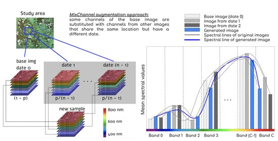
This paper proposes a novel MixChannel augmentation method aiming to address robustness for multispectral satellite (Sentinel) images. We enlarge the training dataset generating new samples artificially with the following procedure. The method is based on substituting bands from original images with the same bands from images of another date covering the same area. While all available images are used during training, only a single image is required for inference time. For this study, only summer images of the active vegetation period are used for conifer and deciduous species classification. We trained CNN models with different architectures to compare the proposed method with the standard augmentation techniques. The result of our MixChannel augmentation consistently outperforms commonly used normalization and augmentation strategies.

The main contributions of this paper are:

• We showcase the problem of poor generalization of CNNs for multispectral satellite images of middle resolution.
• We propose a simple and efficient augmentation scheme that improves CNN model generalization for multispectral satellite images.
• We test the proposed method on conifer and deciduous forest types classification and show that our approach outperforms state-of-the-art solutions.
• We show that the MixChannel approach can be efficiently combined with other methods to achieve the synergy effect.

2. Materials and Methods

2.1. Study Area and Dataset

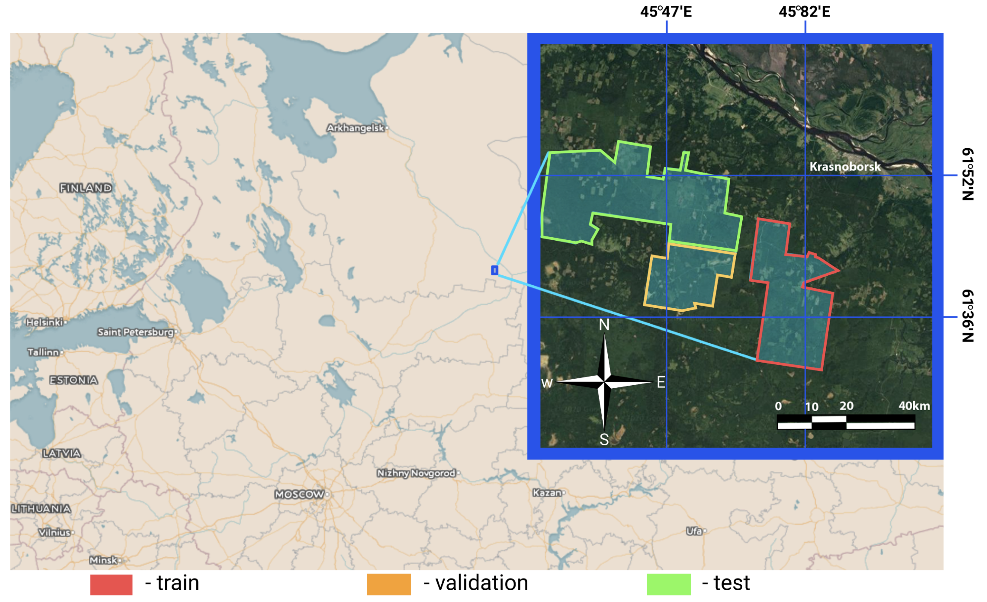
The study area is located in the Arkhangelsk region of northern European Russia with coordinates between ${45}^{°}{16}^{\prime }$ and ${45}^{°}{89}^{\prime }$ longitude and between ${61}^{°}{31}^{\prime }$ and ${61}^{°}{57}^{\prime }$ latitude that belongs to the middle boreal zone (Figure 1). The total area is about $200.000$ hectares. The climate in the region is humid. The warmest month with a temperature of 17 ${}^{°}$C is July. The region’s topography is flat, with a height difference between 170 and 215 m above sea level [16]. The main species present in the region are spruce, aspen, and birch.

For the study, we used forest inventory data collected according to the official Russian inventory regulation [17]. These data were organized as a set of individual stands with appropriate characteristics based on the assumption that the stand was homogeneous. We used such a characteristic as dominant species and canopy height for an additional experiment. Thus, inventory data were converted in a raster map of dominant conifer and deciduous classes and a raster with height values. The statistics of the markup data are presented in

Table 1. Dataset statistical characteristics for conifer and deciduous classification in hectares.

	Training	Validation	Testing	Full Dataset
Conifer	10,000	5000	14,000	29,000
Deciduous	10,000	5000	14,000	29,000

. The assumption on homogeneous means that for particular stands defined as conifer or deciduous dominant types, these individual stands can contain another class representative (but less than $50\%$). We excluded from the study non-forest areas and areas with the equivalent conifer and deciduous composition.

2.2. Satellite Data

The data source used in this paper is Sentinel-2 satellite multispectral images. Sentinel-2 satellite is a part of the Sentinel program with a mission focusing on high-resolution landcover monitoring. It was launched in 2015. Sentinel includes 13 spectral bands with a spatial resolution of 10, 20, and 60 m.

For the forest classification task, we selected images over the vegetation period between the years 2016 and 2019 close to the date of taxation. The study region is boreal forests with high cloud coverage during a year; therefore, the number of appropriate imageries was severely limited. The available image IDs selected for the study are presented in

Table 2. Sentinel images used in this study. Date format is: month, day, year.

	Image ID	Date (Month.Day.Year)
0	L2A_T38VNP_A016606_20180827T083208	08.27.18
1	L2A_T38VNP_A010986_20170730T082009	07.30.17
2	L2A_T38VNP_A005695_20160725T082012	07.25.16
3	L2A_T38VNP_A007297_20180730T081559	07.30.18
4	L2A_T38VNP_A015748_20180628T082602	06.28.18
5	L2A_T38VNP_A013017_20190903T081606	09.03.19

.

We downloaded Sentinel data in L1C format from EarthExplorer USGS [18] and preprocessed them using Sen2Cor [19] to level L2A Bottom of Atmosphere (BoA) reflectance. The pixel values were in the range [0, 10,000]. We used the $B02,B03,B04,B05,B06,B07,B08$, $B11,B12$, and $B8A$ bands [15]. The bands at 20 m resolution were resampled to 10 m resolution before classification using the same procedure discussed in [5].

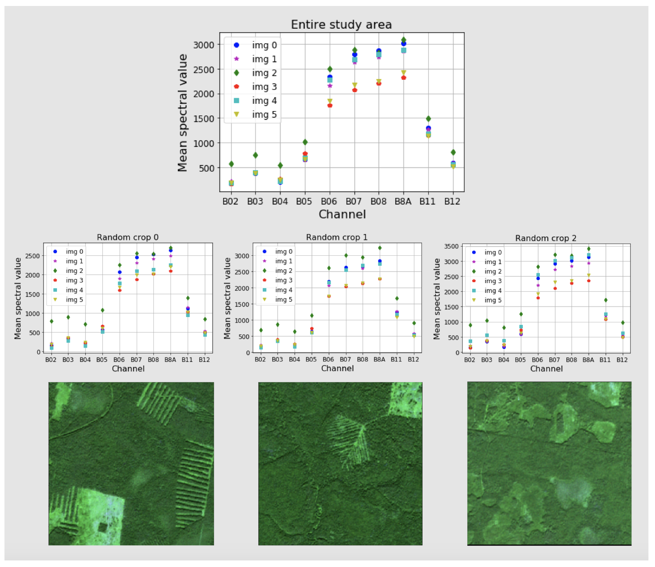
The average values for each channel and each image within forested areas are presented in Figure 2. Here, in the plot for the entire study area, it is shown that the distribution of the mean values for images changes drastically. Even images of the same day but one year apart (images with IDs 1 and 2 for the 30 July 2017, and 2018 respectively) have markedly different mean spectral values. Moreover, for each band, changes are not equivalent. Figure 2 also presents three random crops $200\times 200$ pixels each. It is shown that depending on a particular area, the mean values for each band change. Therefore, it is impossible to bring auxiliary training data within the same image distribution using linear transformations or noise.

For classification tasks using CNN, image values are often brought to the interval from 0 to 1 [20,21]. It can be done using different approaches. The first approach is to divided by the maximum value such as in [22]. In our case, this values is 10,000 (the maximum physical surface reflectance value for Sentinel-2 in level L2A):

$$\begin{array}{c}\hfill I^{\prime }=I/10,000.\end{array}$$

(1)

Another way is to normalize data by the min–max normalization technique. In satellite remote sensing domain, it was used in [23] and aims to reduce noise of each channel:

$$\begin{array}{c}\hfill m=max(0,mean(I)-2\ast std(I\left)\right),\end{array}$$

(2)

$$\begin{array}{c}\hfill M=min\left(max\right(I),mean(I)+2\ast std(I\left)\right),\end{array}$$

(3)

$$\begin{array}{c}\hfill I^{\prime }=(I-m)/(M-m),\end{array}$$

(4)

where $mean,std$ are the mean and standard deviation of the image. In Equations (2) and (3), we calculate m and M (minimum and maximum of the preserved dynamic range). In Equation (4), values are scaled to 0 and 1 linearly.

We used both normalization techniques for evaluating our proposed approach (see Section 2.4).

2.3. Baseline Description

We solve the image semantic segmentation task where a CNN model is trained to create an output map with target classes for each pixel by processing a multispectral input image. Therefore, the output consists of pixels for which forest types are assigned. The batch for model training is formed as follows. For each patch in a batch, one image is chosen from the image set, and a patch of predefined size is cropped randomly. The batch and the patch sizes are presented in Section 2.6. A patch consists of 10 multispectral normalized bands, and it is used as a ten-layer input for a CNN model instead of the usually used three-layer input tensor. For model training, namely model loss function computing, masks with target values are given for each patch. The CNN architecture for the baseline model is U-Net [24].

2.4. MixChannel Augmentation

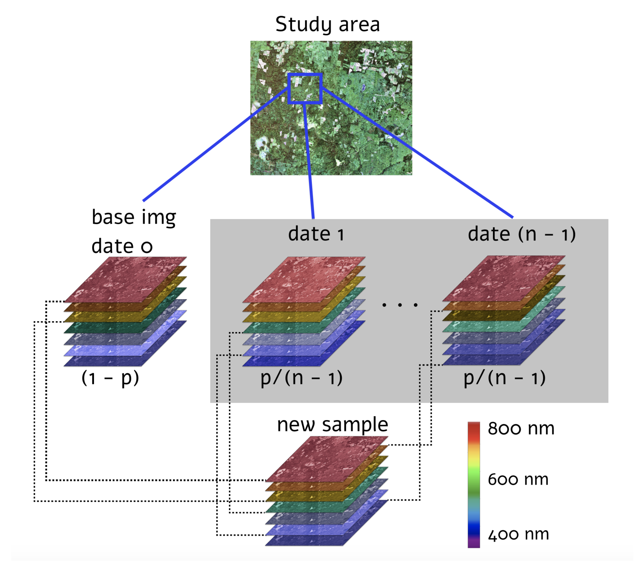
The proposed MixChannel augmentation algorithm operates by substituting some channels of the original image by channels from the other images that cover the same territory (Algorithm 1). MixChannel takes the set of images of the exact location, chooses one as an anchor image, and with the predefined probability substitutes some channels of the anchor image with the matching channels from non-anchor images from the same set. The workflow of the developed augmentation algorithm, in particular, the creation of the new data sample, is schematically presented in Figure 3.

Algorithm 1: MixChannel $\mathcal{T}(S,\acute{P})$

$\mathcal{T}\left(\right)$ is the MixChannel algorithm; $S,\#S\ge 1$ is the set of images covering the same area; $P=\{p_0,p_1,\cdots ,p_{C-1}\},p\sim \mathcal{U}\left([0,1]\right)$ is the set of probabilities to substitute each channel; $I,I\in S$ is the anchor image; C—is the number of channels in images; $R\sim \mathcal{U}\left(\right[0,1\left]\right)$ is a random variable from the uniform distribution; $I_C$ is the c-th channel of the image I; letters with the stroke sign denote temporal variables.   

The probability choice of channel substituting is an essential parameter of the algorithm to be studied. Therefore, we considered different probabilities with the step of $0.1$. The range was set from 0 to $0.7$ where 0 probability is equal to the absence of the MixChannel augmentation and defined as a baseline. To compare the proposed augmentation with other approaches, we conducted the following experiments (see the short summary of experiments in the

Table 3. Experiments description.

No.	Method	Description
1	Baseline	Without any data transformations or aggregations (except geometrical).
2	Baseline + height	Add extra input layer with height values.
3	Channel normalization	Use normalization defined in Equation (4).
4	Average-channel	Aggregate images for various dates by averaging.
5	Channel-dropout	Substitute random channels with zero values.
6	Color jittering	Multiply each channel by a random value.
7	MixChannel	Our approach.
8	MixChannel + height	Add extra input layer with height values.

):

• Average-channel. This experiment is based on the approach proposed for multispectral Sentinel data in [10]. The idea of the method is described in Section 1. For each pixel of the particular band, the corresponding value is averaged within all images that cover the same territory.
• Channel-dropout. In this experiment, we used augmentation described in [25] where it was proposed for RGB images. It aims to prevent a CNN model from overfitting for particular data. Our study implemented this approach by substituting each channel with the predefined probability by zero values. We investigated different probabilities in the range from 0 to $0.5$ with the step of $0.1$.
• Color jittering. Color jittering [26] is commonly used for RGB image augmentation. In the color jittering experiment, we multiply values in each band by the random value (fixed within each band) in the range of 0.8–1.2. The approach aims to add variability to the initial data.
• Patching. As an additional experiment, we implemented MixChannel augmentation for patch parts independently. The patch was divided into four equal parts; for each part, channels can be substituted by bands from different images.
• Optimization. In this experiment, we search for the optimal probabilities for band substitution using a greedy optimization approach. The detailed description of the MixChannel optimization procedure is presented in Section 2.8.
• Height adding. In this experiment, we complemented the spectral data with height data and used them both as input data for CNNs. Experiments MixChannel augmentation for data that include height and Baseline + height are described in details in Section 2.5.

For all experiments except channel-normalization, data were normalized using the Equation (1) described in Section 2.2. In the Channel-normalization experiment, we used Equation (4) for data preprocessing. In all experiments, geometrical transformations such as rotation and random flip were applied.

2.5. Height Data for Stronger Robustness

As was previously shown in [22], additional height data can significantly improve model performance in the forest species classification task. Therefore, we conduct further experiments to evaluate extra height data importance for model robustness in new images and territory. We also check the assumption that MixChannel can be efficiently combined with other techniques to achieve the so-called synergistic effect.

For this experiment, height measurements from inventory data were converted into raster by assigning the same height value to each pixel within an individual stand. This layer was normalized by dividing by 100 and clipping into $[0,1]$ range to have the same range as multispectral input data for a CNN model. The obtained layer was stacked to initial input layers to add additional information to our model.

2.6. Neural Networks Models and Training Details

To evaluate the MixChannel approach on different CNN architectures, we considered U-Net [24], U-Net++ [27], and DeeplLab [28]. For all mentioned architectures, we use ResNet-34 [29] encoder. As a base architecture, we choose U-Net. The models’ architecture implementation was based on opensource library [30] and used PyTorch framework [31].

For each model, we set the following training parameters. There were 50 epochs with 32 training steps per epoch and the same for validation. An Adam optimizer [32] with a learning rate of $0.001$, which was reduced after 25 epochs. Early stopping was chosen with the patience of 10. The best model according to the validation score was considered. The batch size was specified to be 16 with a patch size of $256\times 256$ pixels. These sizes were chosen to meet memory restrictions for computing using one GPU. For each model, the activation function for the last layer was Softmax [33]. As a loss function, categorical cross entropy (5) was used such as in [4].

$$\begin{array}{c}\hfill L(X_i,Y_i)=-\sum _{j=1}^C{y}_{ij}\ast log\left(p_{ij}\right),\end{array}$$

(5)

where:

• $X_i$ is an input vector, and $Y_i$ is a corresponding categorical vector with the ground truth;
• C is the number of target classes;
• $y_{ij}$ equals 1 if ith element is in jth class, and 0 otherwise;
• $p_{ij}$ is probability that ith element belongs to jth class.   

The training of all the neural network models was performed at Zhores [34] supercomputer with 16Gb Tesla V100-SXM2 GPUs.

2.7. Evaluation

Cross-validation is an effective technique for machine learning model assessment [35]. It makes model evaluation more reliable. However, in most works for relatively small datasets (where the study area can be covered by a single satellite tile), splitting for testing and training samples is performed only within the same images. Moreover, the cross-validation technique is not so popular for CNN tasks because it requires extra computational resources. In cases of CNN, fixed splitting into testing and training areas is often used [36]. This study implements an image-based cross-validation approach to evaluate CNN model robustness both for new images and territory for a relatively small dataset.

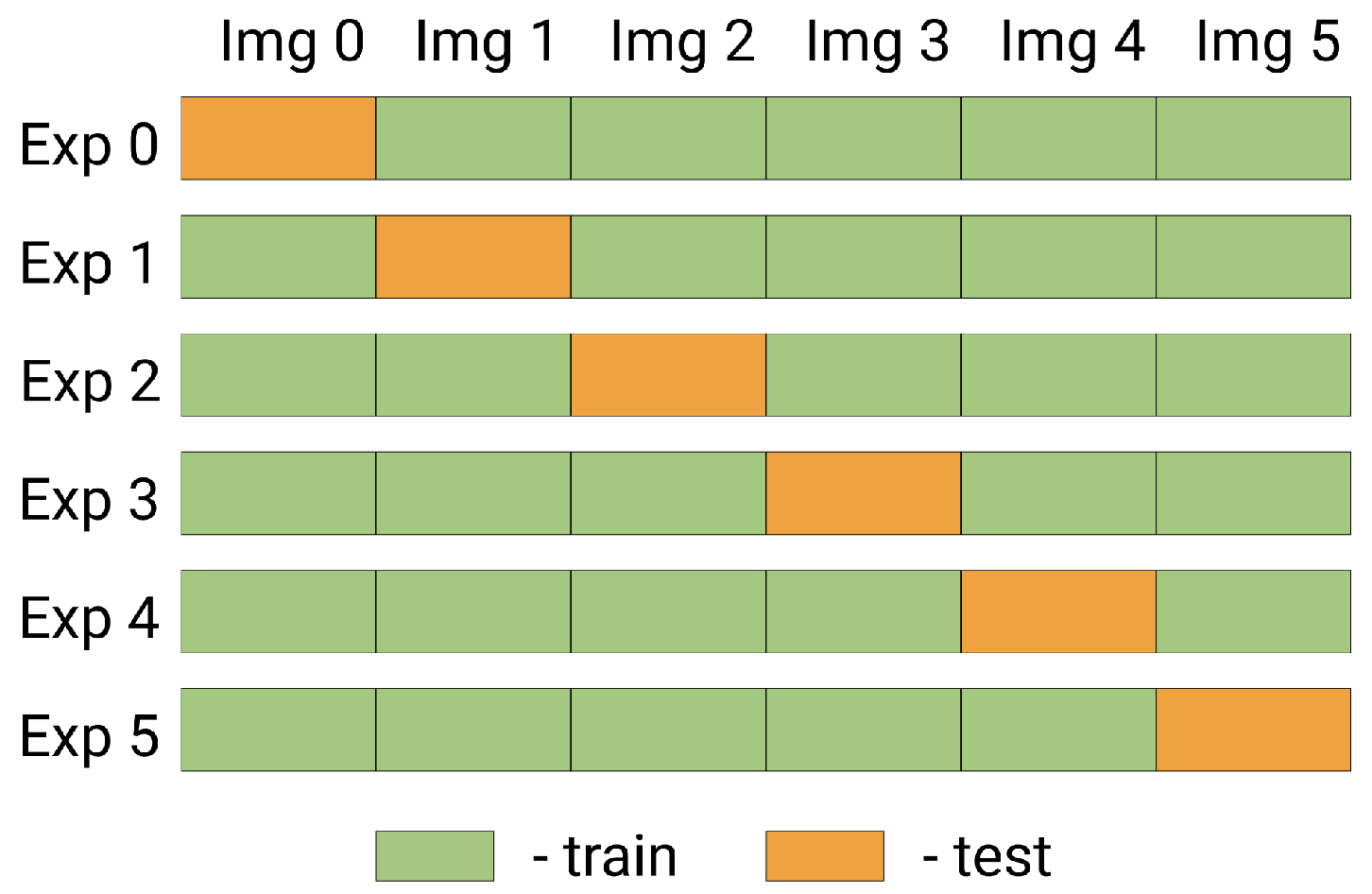
Splitting into folds for cross-validation was organized as follows (Figure 4). Test, train, and validation territories are shown in Figure 1. Six images were used (see Table 2). For each fold, one image was set aside for testing, while the other five images were leveraged to train a model in only the training territory (see Figure 1). Validation was conducted using the same five images but for the validation territory. Thus, the reported result is reliable because it was obtained on unseen images and territories and aggregated across five cross-validation folds.

The model outputs masks of two target classes, which are compared with the ground truth by pixel-wise F1-score (6). It is commonly used in remote sensing tasks [37,38]. F1-score ranges from zero to one, where the higher value represents the better result. For each experiment, a model was trained three times with different random seeds for averaging model performance on different initialization of trained parameters.

$$\begin{array}{c}\hfill F1=\frac{2\ast precision\ast recall}{precision+recall},\end{array}$$

(6)

$$\begin{array}{c}\hfill precision=\frac{TP}{TP+FP},\end{array}$$

(7)

$$\begin{array}{c}\hfill recall=\frac{TP}{TP+FN}\end{array}$$

(8)

where precision and recall are calculated according to Equations (7) and (8), respectively. $TP$ is True Positive (number of correctly classified pixels of the given class), $FP$ represents False Positives (number of pixels classified as the given class while in fact being of other class, and $FN$ is False Negatives (number of pixels of the given class, missed by the method).

2.8. Optimization

The MixChannel algorithm supports changing the probabilities to substitute image channels (see Algorithm 1). Different values of probability have various effects on the final accuracy and robustness of the trained model. Thus, a task of channel substitution probabilities optimization appears. Optimization of these probabilities leads to better results and will be shown in Section 3. However, it should be noted that performance evaluation using each selected probability set requires a full model training cycle. Therefore, it is very computation-intensive to iterate over all possible options. More precisely, it would have exponential complexity with respect to the number of channels.

When computational resources are minimal, the baseline approach assumes that the optimal values for all channels are the same. Then, it is possible to iterate over several probability values and set a single global substitution probability to each channel. The advantage of this approach is that it has constant complexity with respect to the number of image channels because it iterates only over substitution probabilities and does not explore interactions between channels. It allows finding suboptimal probabilities but does not consider that optimal probability may vary severely for some channels. This section proposes a greedy optimization scheme that aims at finding optimal channel substitution probabilities.

Let $\mathcal{J}:H\stackrel{}{\to }\mathcal{R}$ be the objective function. $\mathcal{J}$ maps hyperparameters H that include model, MixChannel parameters and dataset to the resulting $F_1$-score value.

Then, the optimization problem formulates as $P^{☆}=\underset{P}{argmax}\mathcal{J}\left({\theta }^{☆}\right|\mathcal{T}(S,P))$.

The greedy optimization algorithm for MixChannel probabilities tuning operates by iteratively searching for the optimal substitution probability for each channel with other channels’ probabilities fixed to sub-optimal values (Algorithm 2).

Algorithm 2: Greedy MixChannel Optimization

${\theta }^{☆}$—optimal model weights found via the gradient descent algorithm for the defined hyperparameters; q is the the number of probability quantization levels; n is the number of iterations; $p_{max}\le 1$ is the is the highest considered value of probability; r is the the $F_1$-score of the trained model with the considered hyperparameters; v is the the number of images in the dataset covering the same area.

The described optimization algorithm considers the effect of each channel on every other channel. It can be efficiently applied because it has linear complexity with respect to the number of image channels.

3. Results

This section describes the results of the experiments with MixChannel and compares them with other approaches.

MixChannel Augmentation

Table 4. Mix-channel predictions with different channels replacing probabilities (F1-score). Bold text in each row indicates the best result for the model.

Model	Probabilities	0 (Baseline)	0.1	0.2	0.3	0.4	0.5	0.6	0.7
U-Net	Test image 0	0.8	0.762	0.79	0.8	0.77	0.813	0.815	0.795
	Test image 1	0.607	0.606	0.59	0.605	0.58	0.611	0.625	0.59
	Test image 2	0.86	0.829	0.83	0.81	0.835	0.84	0.826	0.825
	Test image 3	0.849	0.814	0.825	0.82	0.815	0.83	0.825	0.83
	Test image 4	0.675	0.733	0.76	0.745	0.725	0.771	0.775	0.77
	Test image 5	0.381	0.72	0.71	0.685	0.685	0.77	0.775	0.655
	Average	0.696	0.744	0.75	0.744	0.735	0.77	0.77	0.74
	Standard deviation	0.17	0.073	0.082	0.076	0.086	0.077	0.069	0.09
Deeplab	Test image 0	0.804	0.793	0.784	0.803	0.817	0.805	0.806	0.813
	Test image 1	0.614	0.631	0.615	0.633	0.633	0.636	0.615	0.596
	Test image 2	0.855	0.811	0.824	0.829	0.832	0.833	0.829	0.828
	Test image 3	0.851	0.834	0.82	0.824	0.812	0.809	0.821	0.823
	Test image 4	0.697	0.76	0.761	0.789	0.774	0.771	0.777	0.771
	Test image 5	0.38	0.664	0.758	0.784	0.722	0.742	0.759	0.736
	Average	0.7	0.749	0.76	0.777	0.765	0.766	0.768	0.761
	Standard deviation	0.167	0.076	0.069	0.066	0.069	0.066	0.0725	0.08
U-Net++	Test image 0	0.79	0.803	0.819	0.824	0.825	0.814	0.817	0.793
	Test image 1	0.49	0.639	0.61	0.618	0.64	0.648	0.605	0.609
	Test image 2	0.861	0.837	0.832	0.811	0.837	0.834	0.837	0.821
	Test image 3	0.851	0.826	0.823	0.822	0.809	0.83	0.828	0.814
	Test image 4	0.6	0.795	0.795	0.765	0.739	0.789	0.775	0.778
	Test image 5	0.38	0.761	0.64	0.735	0.768	0.719	0.774	0.7
	Average	0.66	0.777	0.753	0.762	0.769	0.772	0.773	0.752
	Standard deviation	0.185	0.066	0.091	0.072	0.067	0.069	0.079	0.075

presents details of MixChannel performance. Considering the small number of available training samples, Table 4 shows cross-validation results to increase the reliability of the score. Each model is trained on five training images and is validated on the remaining one image. Columns represent a single global substitution probability, set to each channel. Zero probability means that the MixChannel algorithm is not applied. For a more straightforward interpretation, results for each model aggregated to show average and standard deviation. Bold font highlights the best result for each model. It should be noted that a better model must have a higher F1-score but a lower standard deviation.

The baseline model shows poor performance for particular images (Figure 5). It leads to a low average score ($0.696$) and a high standard deviation ($0.17$) (see Table 4). The model with the same CNN architecture, namely U-Net, but trained using the proposed MixChannel augmentation, beats the baseline approach confidently. For the best substituting probability, it achieves an F1-score of $0.77$ for U-Net architecture. Moreover, the model performance for each test image became more stable. One of the outstanding results is that, for some cases, by using MixChannel augmentation we were able to double the scores. For example, an image with ID 5 was complex for the baseline approach (F1-score $0.381$) and after application of MixChannel augmentation the F1-score doubled and reached $0.775$. The drop of the average standard deviation from $0.17$ to $0.069$ proves that MixChannel enables better model generalization. We compared different probabilities for channel substituting. For the U-Net model, the best one is $0.6$. However, it is clear that the proposed approach leads to higher results even with not the optimal substitution probability.

To evaluate the MixChannel augmentation for different CNN architectures, we conducted experiments with U-Net (as the base model), DeepLab, and U-Net++. Our approach confirms to be preferable for each architecture choice than the baseline approach trained for the same architecture. Moreover, as shown in Table 4 the best score for each architecture is approximately equals to $0.77$. However, the best probability for channel substituting differs: for U-Net, it is $0.6$, for U-Net++ $0.1$, and for DeepLab, it is $0.3$. Unfortunately, we cannot expect the optimal substitution probability to be the same for each model because it is a hyperparameter, and therefore should be tuned for each new case. Every model represents features differently, and augmentation affects these representations differently.

We compared MixChannel performance with the popular solutions for multispectral data. The first experiment was focused on the standard normalization techniques implemented to enhance image spectral properties. As presented in

Table 5. MixChannel comparison with other approaches. Predictions for U-Net models (F1-score). Results of MixChannel application are in blue. Bold text indicates the best result that was obtained by application of MixChannel with height.

Image #	Baseline	Normali-	Average	Color	Channel	MixChannel	Baseline	MixChannel
		zation	Channel	Jittering	Dropout		with Height	with Height
0	0.8	0.839	0.786	0.806	0.809	0.813	0.812	0.845
1	0.607	0.408	0.495	0.551	0.56	0.611	0.605	0.66
2	0.86	0.79	0.844	0.865	0.806	0.84	0.872	0.85
3	0.849	0.859	0.855	0.853	0.816	0.83	0.879	0.865
4	0.675	0.487	0.67	0.579	0.752	0.771	0.73	0.835
5	0.381	0.685	0.38	0.457	0.778	0.77	0.567	0.8
Average	0.696	0.678	0.672	0.685	0.753	0.77	0.74	0.81
		(−1.8%)	(−2.4%)	(−1%)	(+5.7%)	(+7.5%)	(+4.5%)	(+11%)
Standard	0.17	0.175	0.179	0.162	0.089	0.077	0.12	0.069
deviation		(+0.005)	(+0.01)	(−0.01)	(−0.08)	(−0.1)	(−0.05)	(−0.1)

, image normalization did not lead to F1-score improvement ($0.678$) compared to the baseline ($0.696$) where spectral values were dividing by the max possible value. Another considered approach for multispectral augmentation was Channel-dropout. As shown in

Table 6. Channel-dropout predictions for U-Net with different channels replacing probabilities (F1-score). Bold text indicates the best result that was obtained by application of Channel-dropout.

Probabilities	0 (Baseline)	0.1	0.2	0.3	0.4	0.5
Test image 0	0.8	0.802	0.802	0.809	0.794	0.761
Test image 1	0.607	0.57	0.576	0.56	0.504	0.55
Test image 2	0.86	0.814	0.81	0.806	0.791	0.775
Test image 3	0.849	0.804	0.803	0.816	0.791	0.624
Test image 4	0.675	0.752	0.753	0.752	0.756	0.737
Test image 5	0.381	0.689	0.739	0.778	0.766	0.733
Average	0.696	0.738	0.747	0.753	0.733	0.696
Standard deviation	0.17	0.086	0.081	0.089	0.1	0.0816

, it outperforms the baseline model with the best F1-score of $0.753$. However, it still does not achieve MixChannel’s results. We also compared our approach with channel averaging. As presented in Table 5, it did not improve the baseline model results achieved $0.672$ F1-score. Color jittering also did not outperform MixChannel (F1-score $0.685$).

Experiments with additional height data are presented in Table 5. Both for the baseline and MixChannel approaches, it leads to the higher results. For MixChannel F1-score improves from $0.77$ to $0.81$, while for the baseline, F1-score increases from $0.696$ to $0.74$.

In this section above, we showed that the MixChannel algorithm consistently improves model accuracy even with default substitution probabilities. Then, we showed that it is possible to obtain better results tuning a single global probability for each channel (Table 4). Our further experiments show that Algorithm 2 allows finding optimal substitution probabilities separately for each channel. Our optimization setup is as follows. We used the U-Net model; two algorithm iterations n; initial probability values $P=\{0.5,0.5,\dots ,0,5\}$; the highest probability value $p_{max}=0.7$; the number of considered probability values $v=8$. It gives us 160 model training loops in total and increased the previous best result by $1\%$ from $0.777\%$ to $0.791$. It is a minor improvement, but it shows that MixChannel can be tuned further. However, for the practical application, we suggest using global probability tuning because it can noticeably increase model accuracy in a few iterations and can be performed in a parallel fashion.

4. Discussion

Usually, in the remote sensing domain, we do not have a sufficient amount of well-labeled training data for solving particular tasks. The main limitation in getting more data for boreal regions is cloud coverage. Obtaining new labeled data is a time-consuming and costly process because it is often necessary to conduct field-based measurements. Therefore, it is practically reasonable to find techniques that will allow us to enhance the existing image datasets in order to obtain better results in CV models with minimal additional enforces. One of the commonly-used approaches for enhancing the dataset characteristics is image augmentation. However, as is shown above, the standard augmentation techniques are not able to principally improve the scores of trained on multispectral data models. Thus, it is natural to use the distinctive feature of multispectral image data, namely different spectral channels. We showed that generic image augmentations that include color jittering and changing brightness do not ensure robustness for new multispectral images (Table 5). Randomly changing color values in different channels pushes the augmented image out of the distribution of initial images. It may lead to better model robustness against noise but does not ensure better model generalization. As shown in [39], image augmentations that better suit the distribution of the original dataset provide better model performance than augmentations that push images out of distribution. However, it is challenging to preserve the same data distribution with multispectral images because the high number of dimensions makes it difficult to reveal the dependencies between bands.

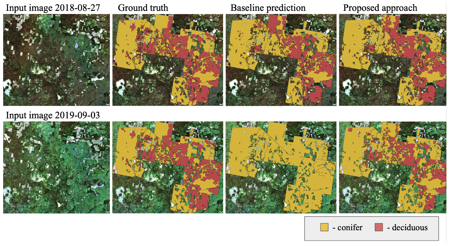
The MixChannel augmentation algorithm proposed in this paper, in contrast, tries to preserve the distribution of the original dataset. It cannot save the joint distributions across all bands, but it saves every separate bands’ distribution. MixChannel substitutes some channels of the anchor image with channels from other images of the same location. The enormous number of possible channel mixing combinations ensures the increase of the number of useful training data images while preserving the distribution characteristics of the dataset. Our experiments show that MixChannel reduced both bias and variance error of all the considered models. The results of the comparison of the predictions for testing and validation areas obtained by baseline models and by using proposed augmentation are presented in Figure 6. From Figure 6 we can visually notice that the proposed approach works better and the prediction results are closer to ground truth. The MixChannel algorithm gains in model performance utilizing the availability of multiple images of the exact location. Therefore, the apparent limitation of the method is the need for more than one image at the same spot. It is suitable in such cases as remote monitoring and continuous stationary imaging. In our investigations, we mainly focus on some image channels substitution with channels from other images. More flexible schemes are also can be considered. It is possible to substitute only some parts (

Table 7. MixChannel for four crop parts (F1-score). Bold text indicates the best result that was obtained by application of MixChannel for four crop parts.

Probabilities	Baseline	0.1	0.2	0.3	0.4	0.5	0.6
Test image 0	0.8	0.798	0.81	0.8	0.798	0.806	0.77
Test image 1	0.607	0.595	0.594	0.624	0.585	0.61	0.616
Test image 2	0.86	0.833	0.83	0.833	0.819	0.835	0.835
Test image 3	0.849	0.828	0.823	0.823	0.82	0.815	0.823
Test image 4	0.675	0.782	0.739	0.77	0.754	0.768	0.77
Test image 5	0.381	0.597	0.674	0.615	0.758	0.71	0.72
Average	0.696	0.738	0.745	0.744	0.756	0.757	0.755
Standard deviation	0.17	0.1	0.0869	0.09	0.08	0.077	0.073

) or patches in a channel by mask instead of the entire channel. Substitution masks can be either based on segmentation masks or random.

We test the MixChannel algorithm using the images with ten channels as an input to CNN models for training them in order to distinguish two classes. In further studies, we will examine the dependency between the number of image channels and the gain of the MixChannel augmentation. It seems promising to test it with three-channel RGB images. The other possible future extension of the current research is to try out more forest species and other classification pipelines (such as a hierarchical approach for species classification described in [22]). Other target classes of vegetation can be studied (such as [3]). For instance, it can be applied for solving some tasks in precision agriculture such as crop boundaries delineation [11]. Such augmentation techniques can be applied for hyperspectral data which is widely used for environmental tasks. The MixChannel algorithm allows for picking different channel substitution probabilities. Our experiments show that the optimal values are not the same for different models. Moreover, the optimal values vary from channel to channel. In practical tasks, we suggest starting with channel substitution probabilities equal to $0.3$ for all channels. Then, depending on the available computational resources, an optimization algorithm can be applied to tune the probabilities if needed.

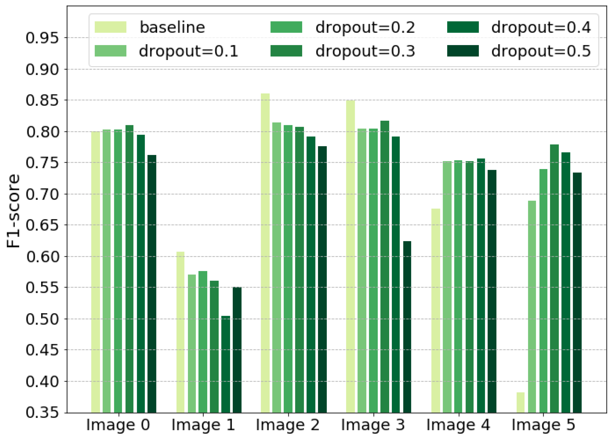
In addition to MixChannel, we show other promising ways to achieve more robust results for CNN model predictions. Channel-dropout demonstrates significantly higher performance than Baseline approach (Table 6, Figure 7). Although Channel-dropout does not outperform MixChannel, it can be applied in cases when just a single multispectral image is available. Both MixChannel and Channel-dropout approaches prevent the model from overfitting on training images and allows extracting relevant information for better predictions. The combination of these augmentations should be studied further. Additional height data is also a powerful way to increase the model robustness (Table 5). It makes the model less sensitive to shifting in spectral distribution. However, height data are not often available.

The design of the MixChannel algorithm uses the variability of the spectrum from image to image. It brings new information when channel values may differ for the target object within the same part of the year. Therefore, this approach is practical for the environmental domain where vegetation characteristics correlate in diverse locations and different years but do not match exactly. In contrast, artificial objects such as buildings remain the same distribution over time and will not benefit in the same way from the MixChannel algorithm. Another limitation arises from the assumption that the objects of interest have no significant changes across the image set. For instance, any crop will differ too much before and after harvesting. Consequently, it is not recommended to apply MixChannel when images for the location are spread across the year, and a CNN model is not supposed to handle such massively different data.

5. Conclusions

This work examines the problem of inconsistency of convolutional neural network generalization in the remote sensing domain. The problem occurs when the training set and the test set of images are from different locations or times of the year. Image exploration shows that even the exact locations at similar dates, but different years, can vary dramatically. It leads to model overfitting on the training set and a drop in performance dramatically on the test set. This problem is crucial when the size of the training set is small. This paper proposes and evaluates a novel image augmentation approach called MixChannel. MixChannel uses multiple multispectral images of the exact location at various dates of the vegetation period to augment the training set. MixChannel was applied to the task of forest types classification in the Northern regions of Russia. This approach shows a noticeable increase in performance with all the tested convolutional neural networks, namely U-Net, Deeplab, and U-Net++. In comparison with other augmentation and preprocessing techniques popular for multispectral images, MixChannel provides better generalization. It is superior in both prediction bias and variance on the unseen test images. The average gain over the baseline solution is $7.5\%$ from $0.696$ F1-score to $0.77$, while the average variance drops more than twice from $0.17$ to $0.077$. Further improvement was achieved by adding auxiliary heights data, giving the overall accuracy of $0.81$. It proves that the proposed approach can be combined with other techniques to get the synergy effect. Our study shows that MixChannel is a promising approach that enables training more precise models for remote sensing in the environmental domain.