Super-Resolution Restoration of Spaceborne Ultra-High-Resolution Images Using the UCL OpTiGAN System

Abstract

We introduce a robust and light-weight multi-image super-resolution restoration (SRR) method and processing system, called OpTiGAN, using a combination of a multi-image maximum a posteriori approach and a deep learning approach. We show the advantages of using a combined two-stage SRR processing scheme for significantly reducing inference artefacts and improving effective resolution in comparison to other SRR techniques. We demonstrate the optimality of OpTiGAN for SRR of ultra-high-resolution satellite images and video frames from 31 cm/pixel WorldView-3, 75 cm/pixel Deimos-2 and 70 cm/pixel SkySat. Detailed qualitative and quantitative assessments are provided for the SRR results on a CEOS-WGCV-IVOS geo-calibration and validation site at Baotou, China, which features artificial permanent optical targets. Our measurements have shown a 3.69 times enhancement of effective resolution from 31 cm/pixel WorldView-3 imagery to 9 cm/pixel SRR.

1. Introduction

Increasing the spatial resolution of spaceborne imagery and video using ground-based processing, or, where feasible, onboard a smart satellite, allows greater amounts of information to be extracted about the scene content. Such processing is generally referred to as super-resolution restoration (SRR). SRR combines image information from repeat observations or continuous video frames and/or exploits information derived (learned) from different imaging sources, to generate images at much higher spatial resolution.

SRR techniques are applicable to images and videos without the usual increased costs and mass, associated with increased bandwidth or larger/heavier optical components, normally required for achieving higher resolution. In particular, enhancing the ultra-high spatial resolution Earth observation (EO) images, or high definition (HD) videos, is an active driver for many applications in the fields of agriculture, forestry, energy and utility maintenance and urban geospatial intelligence. The ability to further improve 30 cm/80 cm EO images and videos into 10 cm/30 cm resolution SRR images and videos will allow artificial intelligence-based (AI-based) analytics to be performed in transformative ways.

This work builds on our previous development from the UKSA CEOI funded SuperRes-EO project, where we developed the MAGiGAN SRR system [1], i.e., Multi-Angle Gotcha image restoration [2,3] with generative adversarial network (GAN) [4]. MAGiGAN was developed to improve the effective resolution of an input lower resolution (LR) image using a stack of overlapping multi-angle (more than 15°) observations. In this paper, we propose a lightweight multi-image SRR system, called OpTiGAN, using optical-flow [5] and total variation [6] image restoration, to replace the extremely computational expensive Gotcha- (Grün-Otto-Chau) [2] based multi-angle restoration [1,3], for continuous image sequences that do not have much change in viewing angles (less than 3°).

We demonstrate the proposed OpTiGAN SRR system with ultra-high resolution Digital Globe^® WorldView-3 panchromatic (PAN) band images (at 31 cm/pixel), obtained through the third-party mission programme of the European Space Agency (ESA), Deimos Imaging^® Deimos-2 PAN band images (at 75 cm/pixel), through EarthDaily Analytics, and Planet^® SkySat HD video frames (at 70 cm/pixel). Image quality evaluation, effective resolution measurements and inter-comparisons of the OpTiGAN SRR results with other SRR techniques were achieved based on a geo-calibration and validation site at Baotou, China [7] (hereafter referred to as Baotou Geocal site). Our quantitative assessments have suggested effective resolution enhancement factors of 3.69 times for WorldView-3 (using five LR inputs), 2.69 times for Deimos-2 (using three LR inputs) and 3.94 times for SkySat (using five LR inputs). An example of the original 31 cm/pixel WorldView-3 image and the 9 cm/pixel OpTiGAN SRR result is shown in Figure 1.

1.1. Previous Work

SRR refers to the process of restoring a higher resolution (HR) image from a single or a sequence of LR images. SRR is traditionally achieved via fusing non-redundant information carried within multiple LR inputs and is mostly achieved nowadays using a deep learning process.

Over the past 30 years, most of the successful multi-image SRR techniques have focused on spatial domain approaches, trying to inverse the degraded imaging process by optimising the image formation and degradation models. Iterative back projection methods were amongst the earliest methods developed for SRR [8,9,10,11,12]. Such methods attempted to define an imaging model to simulate LR images using real observations, then iteratively refine an initial guess of the HR image by comparing its simulated versions of LR images with the provided LR inputs. Later on, maximum likelihood [13,14,15,16,17] and maximum a posteriori (MAP) [6,14,18,19,20,21,22,23,24,25] based approaches attempted to resolve the inverse process stochastically by introducing a priori knowledge about the desired HR image.

On the other hand, machine learning or deep learning-based SRR techniques contain a training step in which the relationship between HR examples and their LR counterparts are learnt. Over the past decade, different deep SRR networks have been proposed, aiming to achieve a higher peak signal to noise ratio (PSNR) [26,27,28,29,30], or aiming to achieve a better perceptual quality [4,31,32,33,34]. These deep SRR networks can be classified as residual-based architectures [35,36,37,38,39], recursive architectures [40,41], attention-based architectures [30,39,42] and GAN-based architectures [4,31,32,33,34]. In particular, GAN-based SRR networks operate by training a generative model and a discriminator model simultaneously (in an alternant manner). In the past few years, GAN and its variations have become fairly popular, especially for perceptual quality driven SRR tasks.

Of particular relevance to this work, we previously proposed two SRR systems, namely, GPT-SRR (Gotcha partial differential equation (PDE) based total variation (TV)) and MAGiGAN SRR, in [1,3], for Mars imagery and EO satellite imagery, respectively, adopting the multi-angle imaging properties and, for the latter one, combining the multi-angle approach with GAN-based inference. GPT-SRR is able to reconstruct the non-redundant information from multi-angle views, based on the MAP framework. MAGiGAN improves upon GPT-SRR and applies a two-stage reconstruction scheme, which combines the advantages from GPT-SRR and GAN SRR and effectively eliminates potential artefacts from using GAN alone. However, the key limitation for [1,3] is that they are both based on the computationally expensive Gotcha process [2], which is not suitable for GPU computing solutions.

In this work, we introduce a new OpTiGAN SRR system that contains modifications and improvements on top of the MAGiGAN SRR system [1], is about 20 times faster in processing speed, uses non-multi-angle observations, e.g., continuous satellite image sequences or video frames, and in particular, is ideal for SRR of ultra-high-resolution (less than 80 cm/pixel) imaging data.

1.2. Datasets

In this work, our test datasets are WorldView-3 (provided by ESA third-party missions from Maxar^®, in 2020), Deimos-2 PAN band images (provided by Deimos Imaging, S.L., in 2021) and SkySat HD video frames (provided by Planet^®, in 2019). The training dataset, used for the GANs, is the Deimos-2 4 m/pixel multispectral (MS) green band and 1 m/pixel (downsampled from 75 cm/pixel) PAN band images (provided by UrtheCast Corp. (now EarthDaily Analytics), in 2018).

The Maxar^® WorldView-3 is the first multi-payload, multi-spectral, high-resolution commercial satellite. WorldView-3 captures images at 31 cm/pixel spatial resolution for the PAN band, 1.24 m/pixel for the MS band, 3.7 m/pixel for the short-wave infrared (SWIR) band and 30 m/pixel for the Clouds, Aerosols, Vapors, Ice and Snow (CAVIS) band, from an operating orbital altitude of 617 km (see https://www.maxar.com/constellation (accessed on 9 June 2021) and https://earth.esa.int/web/eoportal/satellite-missions/v-w-x-y-z/WorldView-3 (accessed on 9 June 2021)) with a swath width of 13.1 km (at nadir). WorldView-3 has an average revisit time of less than one day and is capable of collecting up to 680,000 km² area per day. The WorldView-3 data (for research purposes) are available via application through the ESA site (see https://earth.esa.int/web/guest/pi-community (accessed on 9 June 2021)).

Deimos-2 is a follow-on imaging mission of Deimos-1 for high resolution EO applications owned and operated by the UrtheCast Corp. and Deimos Imaging, S.L. (see https://elecnor-deimos.com/project/deimos-2/ (accessed on 9 June 2021)). Deimos-2 collects 0.75 m/pixel PAN band and 4 m/pixel MS band images with a swath width of 12 km (at nadir) from an orbit at ~600 km. Deimos-2 has a collection capacity of more than 150,000 km² area per day, with a two-day average revisit time worldwide (see https://earth.esa.int/eogateway/missions/deimos-2 (accessed on 9 June 2021)). The MS capability includes four channels in the visible: red, green and blue bands and near-infrared (NIR) band. The Deimos-2 satellite is capable of achieving up to ±45° off-nadir pointing and has a nominal acquisition angle up to ±30° to address particular multi-angle applications.

SkySat is a constellation of 21 high-resolution Earth imaging satellites owned and operated by the commercial company Planet® (see https://www.planet.com/products/hi-res-monitoring/ (accessed on 9 June 2021)). SkySat satellites operates on different orbit altitudes of 600 km, 500 km and 400 km and with different swath width of 8 km (at nadir), 5.9 km (at nadir) and 5.5 km (at nadir), for SkySat-1 and SkySat-2, SkySat-3–SkySat-15, SkySat-16–SkySat-21, respectively. SkySat has an image collection capacity of 400 km² per day and the SkySat constellation has a sub-daily revisit time (6–7 times at worldwide average and 12 times maximum; see https://earth.esa.int/eogateway/missions/skysat (accessed on 9 June 2021)). SkySat captures ~70 cm/pixel resolution still images or HD videos. Full videos are collected between 30 and 120 s (30 frames per second) by the PAN camera from any of the SkySat constellation while the spacecraft pointing follows a target.

2. Methods

2.1. An Overview of the Original MAGiGAN SRR System

The original MAGiGAN SRR system is based on multi-angle feature restoration, estimation of the imaging degradation model and using GAN as a further refinement process. A simplified flow diagram is shown in Figure 2. The overall process of the MAGiGAN SRR system has 5 steps, including: (a) image segmentation and shadow labelling; (b) initial feature matching and subpixel refinement; (c) subpixel feature densification with multi-angle off-nadir view interpolation onto an upscaled nadir reference grid; (d) estimation of the image degradation model and iterative SRR reconstruction; (e) GAN-(pre-trained) based SRR refinement.

MAGiGAN operates with a two-stage SRR reconstruction scheme. The first stage, i.e., steps (a)–(d), provides an initial SRR with an upscaling factor of 2 times of the original LR resolution, followed by the second stage, i.e., step (e), for a further SRR with an upscaling factor of 2 times of the resolution of the intermediate SRR result from the first stage output. A detailed description of the above steps can be found in [1]. It should be noted that, in order to produce sufficient effective resolution enhancement (≥3 times), the input LR images for MAGiGAN must meet one key criteria, which is to contain a wide range (a minimum of 15° and preferably 30°) of multi-angle (off-nadir) views.

2.2. The Proposed OpTiGAN SRR System

In this paper, we propose the OpTiGAN SRR system that is based on the original MAGiGAN framework, but with three key modifications for LR inputs of continuous image sequences or video that do not contain viewing angle changes, to produce similar quality of SRR result (~3 times effective resolution enhancement), compared to MAGiGAN, but with significantly reduced computation time/cost. The flow diagram of the proposed OpTiGAN SRR system is shown in Figure 3, highlighting (in yellow) the modifications, in comparison to the MAGiGAN SRR system. The three modifications are listed as follows.

(a)

Firstly, the shadow labelling module of MAGiGAN is removed in OpTiGAN. Given the LR inputs of continuous image sequence or video frames, the time differences between each LR images are usually minor (i.e., from seconds to minutes), thus shadow/shading differences can be ignored between each LR input. Therefore, there is no need to keep the shadow labelling module in OpTiGAN, whereas when dealing with multi-angle LR inputs using MAGiGAN, the input LR images are normally acquired with much longer time differences (i.e., from days to months).

(b)

Secondly, we compute the dense optical flow between each LR input using the Gunnar Farneback algorithm [5], to produce translation-only transformations of each and every pixel and to replace the computationally expensive Gotcha algorithm, which calculates the affine transformations of each and every pixel. Theoretically, there should be a reduction of the SRR enhancement/quality due to the absence of multi-angle information. We cover this reduction by implementing the third modification, i.e., (c), which is introduced next. In return, by replacing Gotcha, we obtain a ~20 times of speedup.

(c)

Thirdly, we replace the original GAN prediction (refinement) module with the MARSGAN model described in [43], where we demonstrated state-of-the-art single image SRR performance for 4 m/pixel Mars imaging datasets. The network architecture of MARSGAN can be found in [43]. In this work, we re-train the MARSGAN network with the same training dataset used in [44]. The updated GAN module offers improvement to the overall process of OpTiGAN, which complements the fallback introduced in (b).

With the afore-mentioned modifications, OpTiGAN is able to achieve similar SRR enhancement (in comparison to MAGiGAN [1]) in a much shorter (~20 times shorter) processing time, for continuous image sequences and video frames with “zero” (or little) viewing angle changes. The rest of the processing components are the same as MAGiGAN [1]. The overall process of the OpTiGAN SRR system has 5 steps, including: (a) initial image feature matching and subpixel refinement; (b) calculation of dense sub-pixel translational correspondences (motion prior) with optical flow; (c) estimation of the image degradation model using the computed motion prior from (b) and initialisation of an intermediate SRR reconstruction using PDE-TV; (d) MARSGAN (pre-trained) SRR refinement on top of the intermediate SRR output from step (c).

OpTiGAN also operates on a two-stage SRR reconstruction process. In the first stage processing of OpTiGAN, i.e., steps (a)–(c), 2 times upscaling is achieved with the optical-flow PDE-TV, followed by a second stage, i.e., step (d), for a further 2 times upscaling, using the pre-trained MARSGAN model, resulting in a total of 4 times upscaling for the final SRR result.

In particular to the implementation of the optical flow-based motion prior estimation, we use the OpenCV implementation (see https://docs.opencv.org/3.4/de/d9e/classcv_1_1FarnebackOpticalFlow.html (accessed on 9 June 2021)) of the Gunnar Farneback algorithm [5]. This method uses a polynomial expansion transform to approximate pixel neighbourhoods of each input LR image and the reference image (could be any image in the inputs—usually the first one) and then estimates displacement fields from the polynomial expansion coefficients. With dense optical flow, the affine correspondences of local pixel points are simplified with translation-only correspondences. The omnidirectional displacement values from dense optical flow are then passed through to the MAP process (PDE-TV) [1,3], as the motion prior.

Using the two-stage SRR reconstruction scheme (both in MAGiGAN and the proposed OpTiGAN), we found, in [1], that the MAP-based approaches (i.e., the first stage of MAGiGAN/OpTiGAN) are highly complementary with the deep learning-based approaches (e.g., the second stage of MAGiGAN/OpTiGAN), in terms of restoring and enhancing different types of features. In particular, the first stage of the OpTiGAN processing retrieves sub-pixel information from multiple LR images and tends to produce robust restorations (“artefact free”) of small objects and shape outlines, whereas the second stage of the OpTiGAN processing contributes more to the reconstruction of the high-frequency textures. Besides, experiments in [1] and in this paper (see Section 3 for demonstration) have shown that using GAN inference alone, i.e., without the first stage of the OpTiGAN processing, can result in artificial textures or even synthetic objects, whereas using GAN inference on top of an intermediate SRR result produced from a classic MAP-based approach produces the highest effective resolution, in terms of resolvable small objects and edge/outline sharpness and texture details, with the least artefacts.

On the other hand, in the second stage of OpTiGAN processing, we replace the original GAN implementation, which was an optimised version of SRGAN [4], with our recently developed MARSGAN model [43]. This is the same as a general GAN framework, wherein MARSGAN trains a generator network to generate potential SRR solutions and a relativistic adversarial network [32,43,45] to pick-up the most realistic SRR solution. MARSGAN uses 23 Adaptive Weighted Residual-in-Residual Dense Blocks (AWRRDBs), followed by an Adaptive Weighted Multi-Scale Reconstruction (AWMSR) block in the generator network, providing much higher network capacity and better performance, compared to the original SRGAN-based model used in MAGiGAN (see Section 3 for comparisons). Besides, MARSGAN uses a balanced PSNR-driven and perceptual quality-driven [43] loss function to produce high quality restoration while limiting synthetic artefacts. A simplified network architecture of the MARSGAN model is shown in Figure 4. A detailed description of the MARSGAN network can be found in [43].

With the above changes, OpTiGAN operates the best on slowly “drifting” scenes with less than 3° of changes in camera orientations, while MAGiGAN operates the best on “point-and-stare” and/or multi-angle repeat-pass observations with more than 15° of changes in camera orientations.

2.3. Training Details of the MARSGAN Model

In this work, we retrained the MARSGAN model with the Deimos-2 images used in [44], using a similar hyperparameter set-up, as used previously in [43], i.e., batch size of 64, adversarial loss weight of 0.005, same low-level and high-level perceptual loss weight as 0.5, pixel-based loss weight of 0.5 and an initial learning rate of 0.0001, which is then halved at 50 k, 100 k, 200 k and 400 k iterations.

We have re-used the same training datasets as described in [44]. The training datasets were formed from 102 non-repeat and cloud-free Deimos-2 images, including the 4 m/pixel MS green band images (bicubic upsampled to 2 m/pixel for OpTiGAN training) and the 1 m/pixel (downsampled) PAN band images. The 102 resampled (2 m/pixel and 1 m/pixel) Deimos-2 MS green band and PAN band images were then cropped and randomly selected (50% of total samples are reserved) to form 300,512 (32 by 32 pixels) LR training samples and 300,512 (64 by 64 pixels) HR training samples. It should be noted that additional training (for validation and comparison purposes) of the SRGAN, ESRGAN and MARSGAN networks used the original 4 m/pixel MS green band images (without upsampling) and a larger HR sample size (128 by 128 pixels), in order to achieve the unified upscaling factor (4 times) for intercomparisons.

All training and subsequent SRR processing were performed on the latest Nvidia^® RTX 3090 GPU and an AMD^® Ryzen-7 3800X CPU.

It should be noted that the final trained MARSGAN model has a high scalability over different datasets that have different resolutions (from 30 cm to 10 m). Other than the demonstrated ultra-high-resolution datasets, it also works for the 4 m Deimos-2 MS band images and 10 m Sentinel-2 images.

2.4. Assessment and Evaluation Methods

In this work, our target testing datasets are amongst the highest resolution satellite optical data for EO, therefore there is no “reference HR” image available for direct comparison and evaluation. Standard image quality metrics, e.g., PSNR and structural similarity index metric, that require a reference HR image, cannot be used for this work. However, we visually examined and compared the restorations of different artificial targets (i.e., the bar-pattern targets and fan-shaped targets, available at the Baotou Geocal site) in the SRR results against fully measured reference truth (see Figure 5). The smallest bars that were resolvable in the SRR results are summarised in Section 3.

Our initial qualitative assessment was based on two image quality metrics, i.e., the blind/referenceless image spatial quality evaluator (BRISQUE) [46] and the perception-based image quality evaluator (PIQE) [47] scores (for implementation see https://uk.mathworks.com/help/images/image-quality.html (accessed on 9 June 2021)).

Figure 5. Illustration of the artificial optical targets at the Baotou Geocal site. Photo pictures (left) courtesy from [48] and map of the bar-pattern target (right) provided by L. Ma [48] and Y. Zhou [49] (private correspondence, 2021).

Figure 5. Illustration of the artificial optical targets at the Baotou Geocal site. Photo pictures (left) courtesy from [48] and map of the bar-pattern target (right) provided by L. Ma [48] and Y. Zhou [49] (private correspondence, 2021).

In addition, we performed edge sharpness measurements using the Imatest^® software (https://www.imatest.com/ (accessed on 9 June 2021)) to measure the effective resolutions of the SRR results. The Imatest^® edge sharpness measurement calculated the averaged total amount of pixels from 20% to 80% rises of slanted-edge profiles within a given high-contrast area. If the total number of pixels of such profile rises in the SRR image was compared against the total number of pixels involved in its LR counterpart, for the same slanted-edge profile, then their ratio could be used to estimate an effective resolution enhancement factor between the two images (biased to the measured edge in particular). We performed this test using the knife-edge target visible at the Baotou Geocal site (see Figure 5) with multiple slanted-edges and then averaged the resolution enhancement factors, estimated with different slanted-edges, to obtain an averaged effective resolution enhancement factor for the SRR results.

3. Results

3.1. Experimental Overview

The Baotou Geocal site (50 km away from the Baotou city) located at 40°51′06.00″N, 109°37′44.14″E, Inner Mongolia, China, was used as the test site in this study, in order to obtain assessments which can be compared against other published ones. The permanent artificial optical targets (see Figure 5), at the Baotou Geocal site, provided broad dynamic range, good uniformity, high stability and multi-function capabilities. Since 2013, the artificial optical targets have been successfully used for payload radiometric calibration and on-orbit performance assessment for a variety of international and domestic satellites. The artificial optical targets were set-up on a flat area of approximately 300 km², with an average altitude of 1270 m. The Baotou Geocal site features a cold semi-arid climate that has (an average of) ~300 clear-sky days every year, which has made it an ideal site for geo-calibration and validation work. Some illustration photos (courtesy of [48]) of the artificial optical targets, including a knife-edge target, a fan-shaped target and a bar-pattern target, at the Baotou Geocal site, as well as the fully measured reference truth (provided by L. Ma [48] and Y. Zhou [49] in private correspondence) for the bar-pattern target, can be found in Figure 5.

We tested the proposed OpTiGAN SRR system with three ultra-high-resolution satellite datasets, i.e., the 31 cm/pixel WorldView-3 PAN images, the 75 cm/pixel Deimos-2 PAN images and the 70 cm/pixel SkySat HD video frames.

Table 1. Input image IDs for WorldView-3, Deimos-2 and SkySat image/video frames. The first row of the image IDs shows the reference image for multi-image SRR and sole-input for single-image SRR. WorldView-3 Maxar^® image 2020, provided by the European Space Agency; Deimos-2^®: Deimos Imaging, S.L. in 2021; Skysat L1A imagery provided by Planet Labs, Inc.

WorldView-3	Deimos-2	SkySat
18AUG18040034-P2AS-012860253020_01_P006	DE2_PAN_L1C_000000_20171028T032332_20171028T032334_DE2_18196_7323	1256786198.72711825_sc00112_c2_PAN_i0000000246_16bit
18AUG05035334-P2AS-012860253020_01_P007	DE2_PAN_L1C_000000_20161202T032012_20161202T032015_DE2_13299_0195	1256786198.79377627_sc00112_c2_PAN_i0000000247_16bit
18JUL11035419-P2AS-012860253020_01_P009	DE2_PAN_L1C_000000_20180427T032701_20180427T032703_DE2_20882_109E	1256786198.86044383_sc00112_c2_PAN_i0000000248_16bit
18AUG31040658-P2AS-012860253020_01_P005		1256786198.92711139_sc00112_c2_PAN_i0000000249_16bit
20FEB16035612-P2AS-012860253020_01_P004		1256786198.99377990_sc00112_c2_PAN_i0000000250_16bit

shows the input image IDs used in this work. Note that the first row was used as the reference image in case of multi-image SRR processing and it was also the sole-input in case of single-image SRR processing.

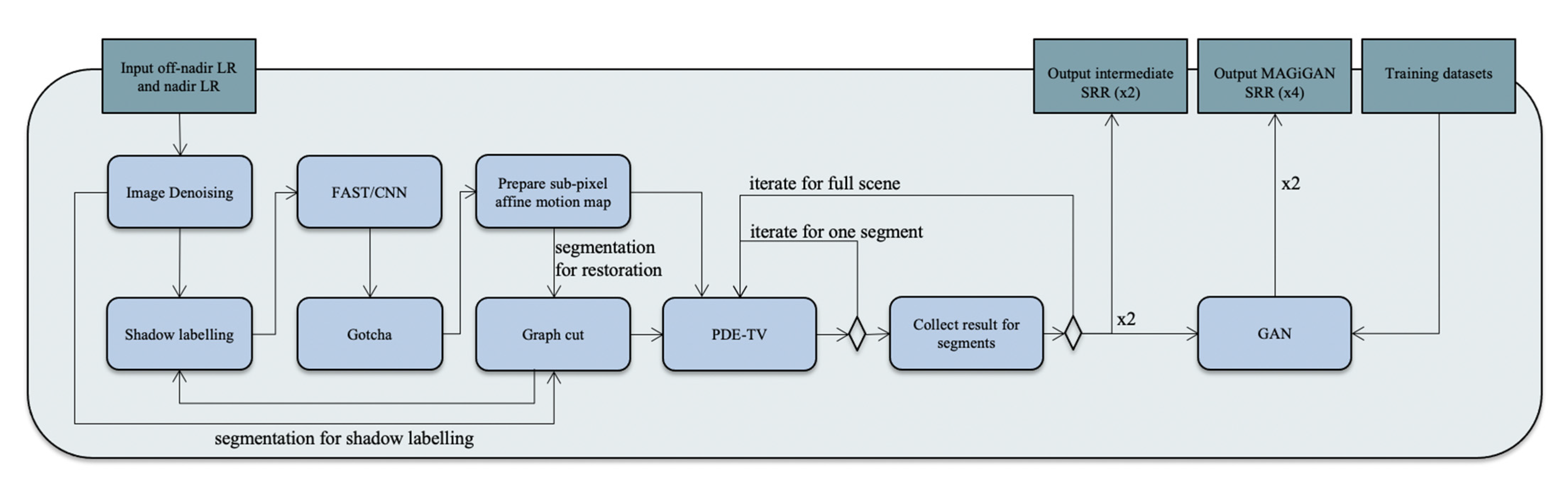
Since MAGiGAN and OpTiGAN require different inputs, i.e., LR images with viewing angle differences and without viewing angle differences, respectively, we are not able to provide results of a comparison of performance between these two SRR systems. However, in this work, we provide intercomparisons against four different SRR techniques. The four SRR techniques include: (1) an optimised version of the SRGAN [4] single-image SRR network that was used in MAGiGAN [1] (hereafter referred to as SRGAN, in all text, figures and tables); (2) ESRGAN [32] single-image SRR network; (3) MARSGAN [43] single-image SRR network, which was also used as the second stage processing of OpTiGAN; (4) optical-flow PDE-TV (OFTV; hereafter referred to as OFTV, in all text, figures and tables) multi-image SRR, which was also used as the first stage processing of OpTiGAN. It should be noted that all deep network-based SRR techniques, i.e., SRGAN, ESRGAN, MARSGAN and OpTiGAN, were trained with the same training datasets, as described in Section 2.3.

3.2. Demonstration and Assessments of WorldView-3 Results

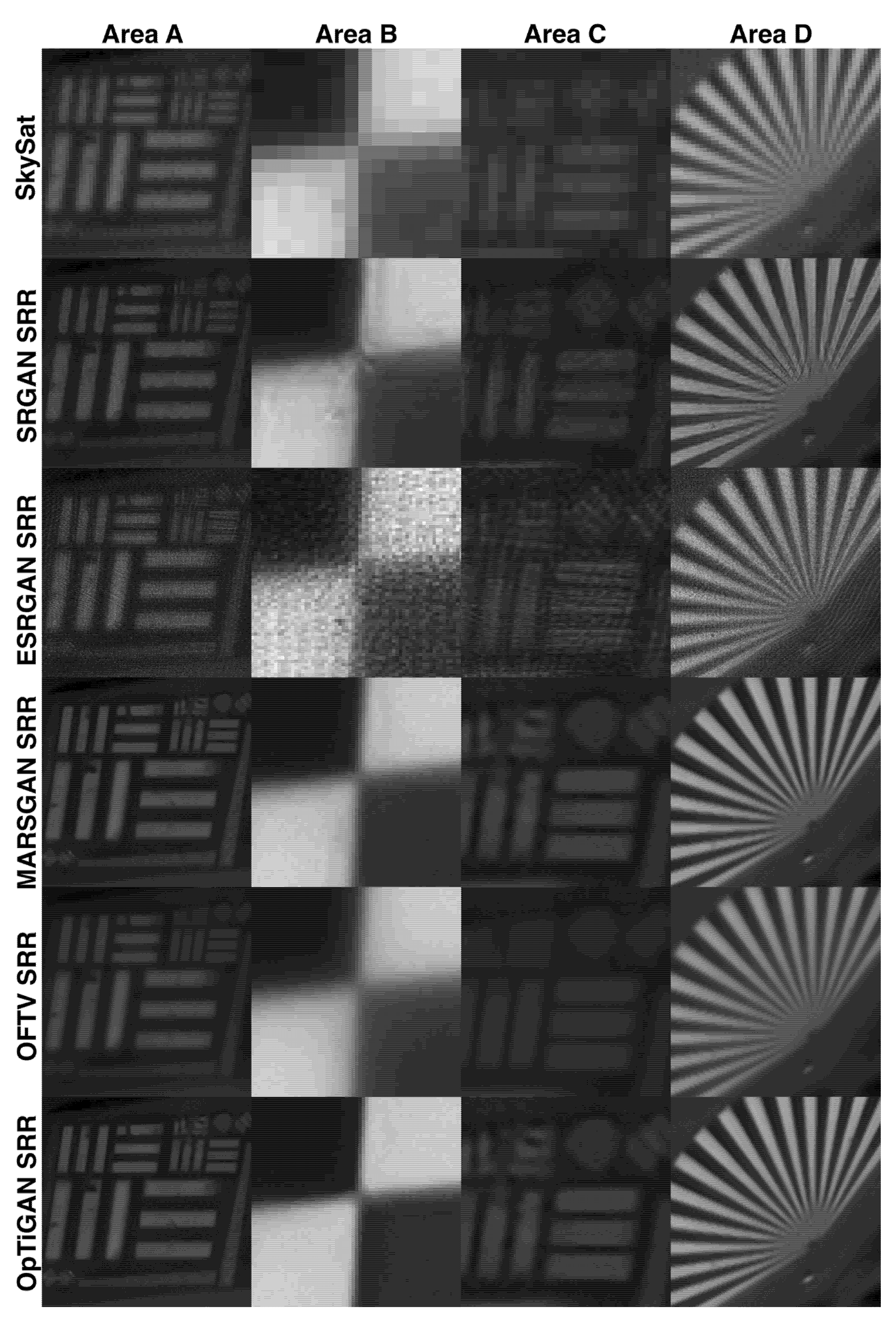
For the WorldView-3 experiments, we used a single input image for the SRGAN, ESRGAN and MARSGAN SRR processing and used five overlapped input images for the OFTV and OpTiGAN SRR processing. Four cropped areas (A–D) covering the different artificial targets at the Baotou Geocal site are shown in Figure 6 for comparisons of the SRR results and the original input WorldView-3 image.

Area A showed the 10 m × 2 m and 5 m × 1 m bar-pattern targets. We can observe that all five SRR results showed good restoration of these larger sized bars. The SRGAN result of Area A showed some rounded corners of the 5 m × 1 m bars, whereas the ESRGAN result showed sharper corners, but with some high-frequency noise. The MARSGAN result showed the best overall quality among the three single-image deep learning-based SRR techniques. In comparison to the deep learning-based techniques, OFTV showed smoother edges/outlines, but with no observable artefact. The OpTiGAN result, which was based on OFTV and MARSGAN, showed the best overall quality, i.e., similar sharpness on edges/outlines/corners, but with no artefact or high-frequency noise.

Area B showed the central area of the knife-edge target. All three deep learning-based techniques showed sharp edges of the target; however, the SRGAN result appeared to demonstrate some artefacts at the centre corner and some artefacts at the edges, ESRGAN showed some high-frequency noise, whilst MARSGAN had some artefacts at the edges. OFTV showed a blurrier edge compared to SRGAN, ESRGAN and MARSGAN, but it showed the least number of artefacts. OpTiGAN had shown sharp edges that were similar to ESRGAN and MARSGAN, but with much less noise and artefact.

Area C showed a fan-shaped target. We can observe that all five SRR results showed good restoration of the target at mid-range radius. The MARSGAN and OpTiGAN results showed reasonable restoration at the centre radius, i.e., by the end of the target, with only a few artefacts at the centre and in between each strip pattern. ESRGAN also showed some reasonable restoration at small radius, but the result was much noisier compared to MARSGAN and OpTiGAN. SRGAN showed obvious artefacts at small radius. OFTV did not show as much detail as the other techniques, but, instead, it showed no observable noise or artefact. In terms of sharpness, ESRGAN, MARSGAN and OpTiGAN had the best performance. However, MARSGAN and OpTiGAN had less noise compared to ESRGAN, with OpTiGAN showing the least artefacts among the three.

Area D showed a zoom-in view of the larger 10 m × 2 m bar-pattern targets along with multiple smaller bar-pattern targets with size ranges from 2.5 m × 0.5 m, 2 m × 0.4 m, 2 m × 0.3 m, 2 m × 0.2 m, to 2 m × 0.1 m, from bottom-right to top-right (see Figure 5). We can observe that all five SRR techniques were able to restore the 2.5 m × 0.5 m bars reasonably well, despite the SRGAN results showing some tilting. The tilting artefact became more severe for the 2 m × 0.4 m bars for SRGAN and the bars were not clearly visible at the 2 m × 0.4 m scale and above. ESRGAN showed clear individual bars at 2 m × 0.4 m, but all of them had the same tilting artefact. In the MARSGAN result, we could observe smaller bars up to 2 m × 0.3 m, but still with artefacts, i.e., tilting and wrong shapes. OFTV showed smoother edges of the bars, but with very little artefact. The shapes and angles of the small bar strips, at the right side of the crop, were more correct (refer to Figure 5) with OFTV and the smallest resolvable bars were in between 2 m × 0.4 m and 2 m × 0.3 m. Finally, the OpTiGAN result showed the best restoration of the 2 m × 0.4 m bars compared to the other four SRR results. The smallest recognisable bars were between 2 m × 0.3 m and 2 m × 0.2 m, for OpTiGAN. However, OpTiGAN still had some artefacts for bars at the 2 m × 0.3 m scale that were similar to the MARSGAN result.

In

Table 2. BRISQUE and PIQE assessments of the WorldView-3 image and its SRR results at Baotou Geocal site.

	WorldView-3	SRGAN	ESRGAN	MARSGAN	OFTV	OpTiGAN
BRISQUE	45.2338	37.9340	28.9244	25.7153	38.9264	31.8876
PIQE	73.9336	57.1820	16.1597	22.3267	32.2479	24.3363

, we show the BRISQUE and PIQE image quality scores (0–100, lower scores representing better image quality) that were measured from the full-image (see Supplementary Materials for the full-image) at the Baotou Geocal site. We can observe improvements in terms of image quality from all five SRR techniques. MARSGAN achieved the best image quality score from BRISQUE, whereas ESRGAN achieved the best image quality score from PIQE. The image quality scores for OpTiGAN were close to ESRGAN and MARSGAN. The lower image quality scores reflected better overall image sharpness and contrast. However, since this measurement did not count for incorrect high-frequency texture, incorrect reconstruction of small sized targets and synthetic artefacts, the better scores do not reflect absolute better quality of the SRR results. More quantitative assessments are given in

Table 3. Summary of slanted-edge measurements as shown in Figure 7, for total pixel counts for 20–80% rise of the edge profile and the suggested effective resolution enhancement factor comparing to the input WorldView-3 image (upscaled by a factor of 4 for comparison).

	WorldView-3	SRGAN	ESRGAN	MARSGAN	OFTV	OpTiGAN
Edge-1 pixel counts	5.31 pixels	3.38 pixels	3.85 pixels	2.96 pixels	3.57 pixels	1.80 pixels
Edge-1 enhancement factor	-	1.57 times	1.38 times	1.79 times	1.49 times	2.95 times
Edge-2 pixel counts	4.25 pixels	2.31 pixels	2.38 pixels	1.16 pixels	2.50 pixels	1.14 pixels
Edge-2 enhancement factor	-	1.84 times	1.79 times	3.66 times	1.7 times	3.73 times
Edge-3 pixel counts	4.08 pixels	2.40 pixels	2.56 pixels	1.04 pixels	2.89 pixels	0.93 pixels
Edge-3 enhancement factor	-	1.7 times	1.59 times	3.92 times	1.41 times	4.39 times
Average enhancement factor	-	~1.7 times	~1.59 times	~3.12 times	~1.53 times	~3.69 times

and

Table 4. Summary of the effective resolution derived from Figure 7 and Table 3, the smallest resolvable bar pattern targets observed from the WorldView-3 image and each of the SRR results, in comparison to Figure 5, as well as the number of input images used and computing time for the Baotou Geocal site.

	WorldView-3	SRGAN	ESRGAN	MARSGAN	OFTV	OpTiGAN
Image size	420 × 420 pixels	1680 × 1680 pixels
Spatial resolution	31 cm/pixel	7.75 cm/pixel
Effective resolution	Assuming 31 cm/pixel	18 cm/pixel	19 cm/pixel	10 cm/pixel	20 cm/pixel	9 cm/pixel
Smallest resolvable bar (recognisable)	60 cm	40 cm	40 cm	30 cm	30 cm	20 cm
Smallest resolvable bar (with good visual quality)	80 cm	50 cm	50 cm	50 cm	40 cm	30 cm
Number of LR input used	-	1	1	1	5	5
Computing time	-	<1 s	<1 s	<1 s	~10 min	~10 min

.

It has been the case that in the field of photo-realistic SRR, many SRR techniques present “fancy” images with four times or even eight times of upscaling factor, but their effective resolution never reaches the upscaling factor. In this paper, we present a more quantitative assessment using the Imatest^® slanted-edge measurement for the knife-edge target at the Baotou Geocal site. In Figure 7, we show three automatically detected edges and their associated 20–80% profile rise analysis for each of the input WorldView-3 image, SRGAN SRR result, ESRGAN SRR result, MARSGAN SRR result, OFTV SRR result and OpTiGAN SRR result. The total pixel counts for the 20–80% profile rise of each slanted edge are summarised in Table 3. We divided the total pixel counts of the input WorldView-3 image (upscaled by a factor of 4 for comparison) with the total pixel counts of the SRR results to get the effective resolution enhancement factor for each of the measured edges. Note that the edge sharpness measurements are generally similar but may be different from area to area, even in the same image, thus we averaged three measurements to get the final effective resolution enhancement factor. The average effective resolution enhancement factors are shown in the last row of Table 3.

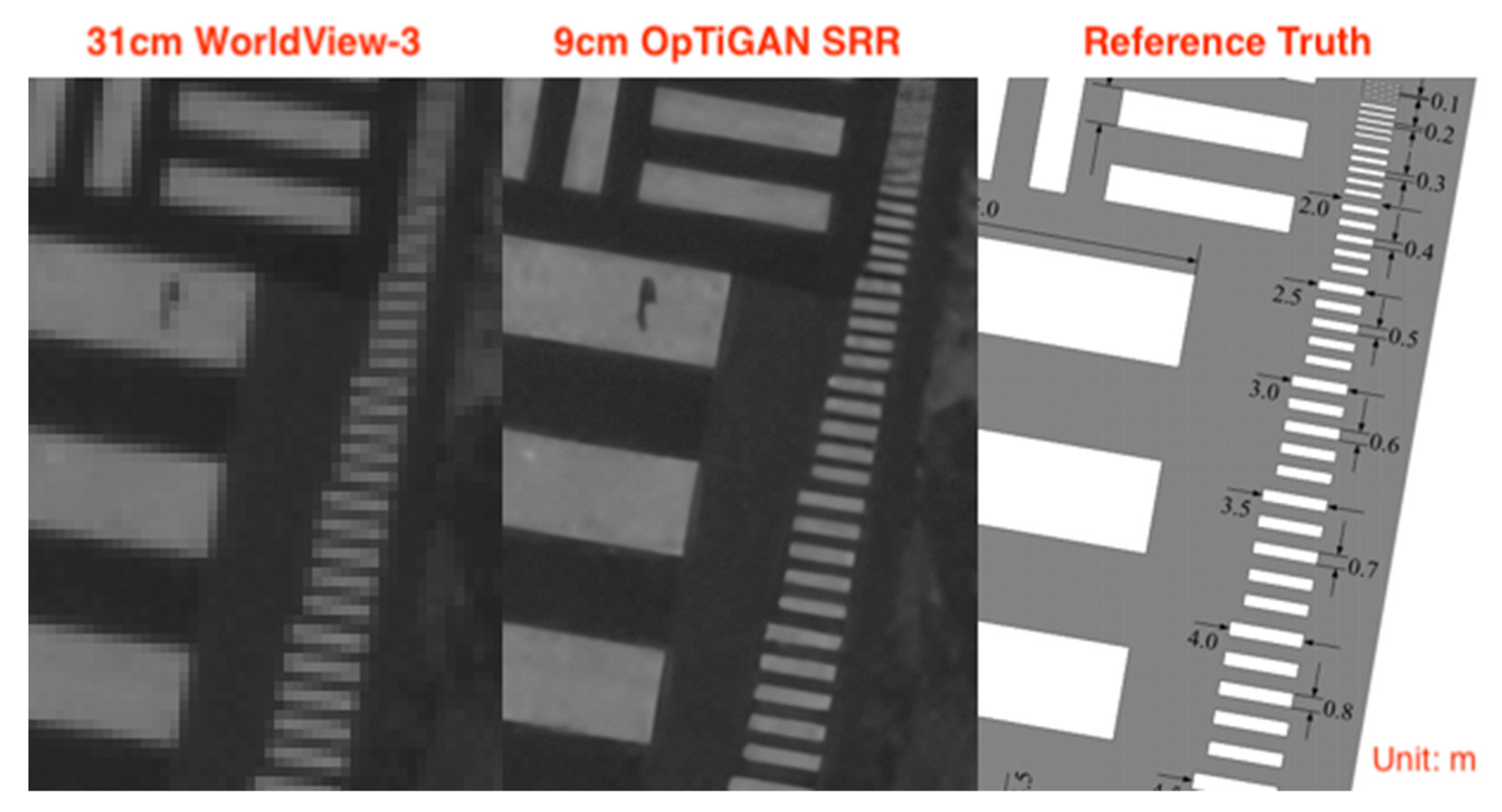
Another quantitative assessment of image effective resolution was achieved via visually checking the smallest resolvable bar targets for each of the SRR results. This is summarised in Table 4. We checked the smallest resolvable bar targets in terms of “recognisable” and “with good visual quality”, where “recognisable” means visible and identifiable and does not count for noise or artefacts and “with good visual quality” means clearly visible with little or no artefacts. We can see from Table 4 that, with a 31 cm/pixel resolution WorldView-3 image, we can resolve 60 cm/80 cm bar targets and, with a 9 cm/pixel OpTiGAN SRR, we can resolve 20 cm/30 cm bar targets. Table 4 also shows the effective resolution calculated from Table 3, along with input and processing information. Note, here, the proposed OpTiGAN system has significantly shortened the required processing time from a few hours to around 10 min for five of 420 × 420-pixel input images in comparison to MAGiGAN [1], which we based the aforementioned modifications on.

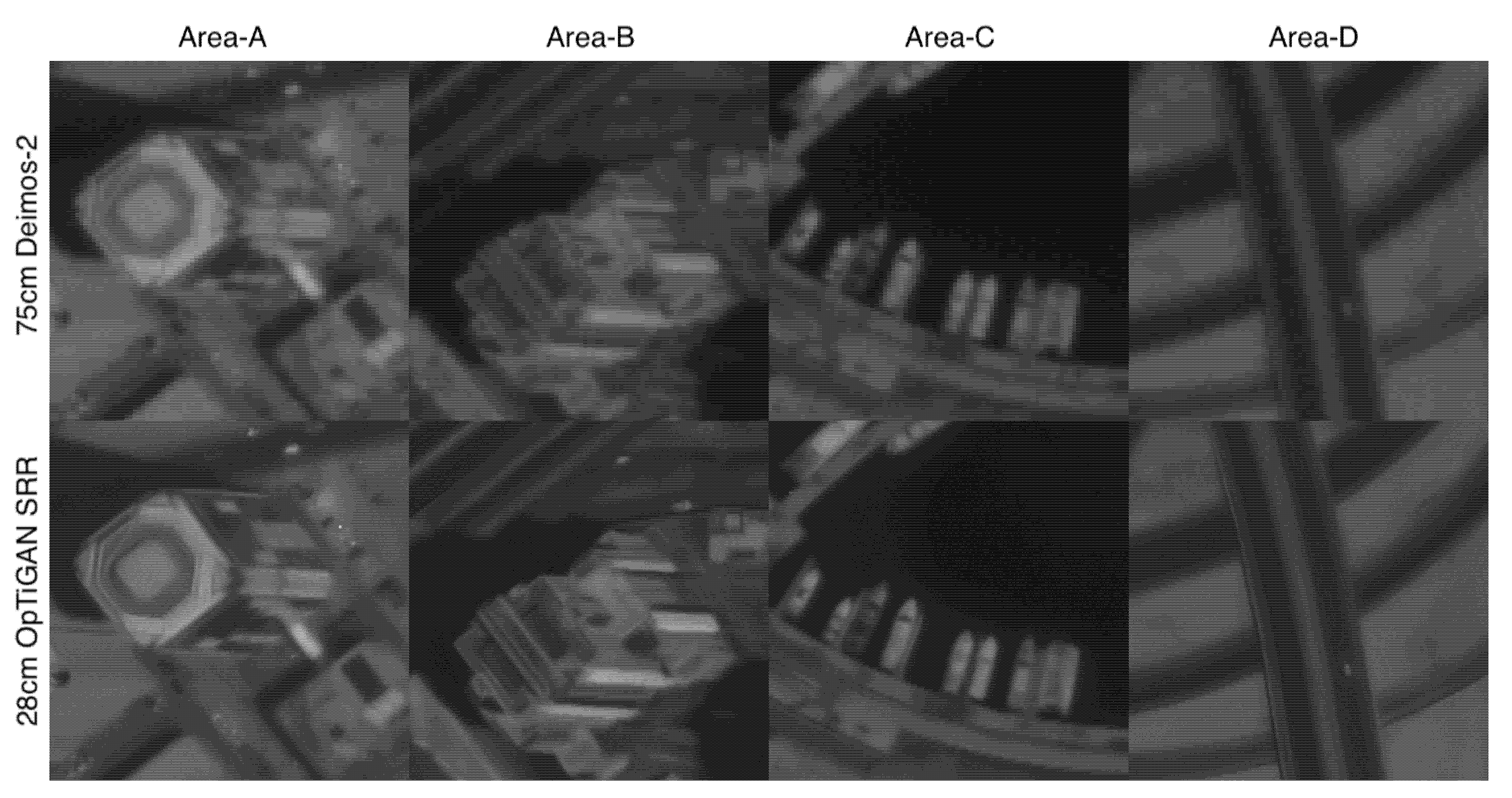
3.3. Demonstration and Assessments of Deimos-2 Results

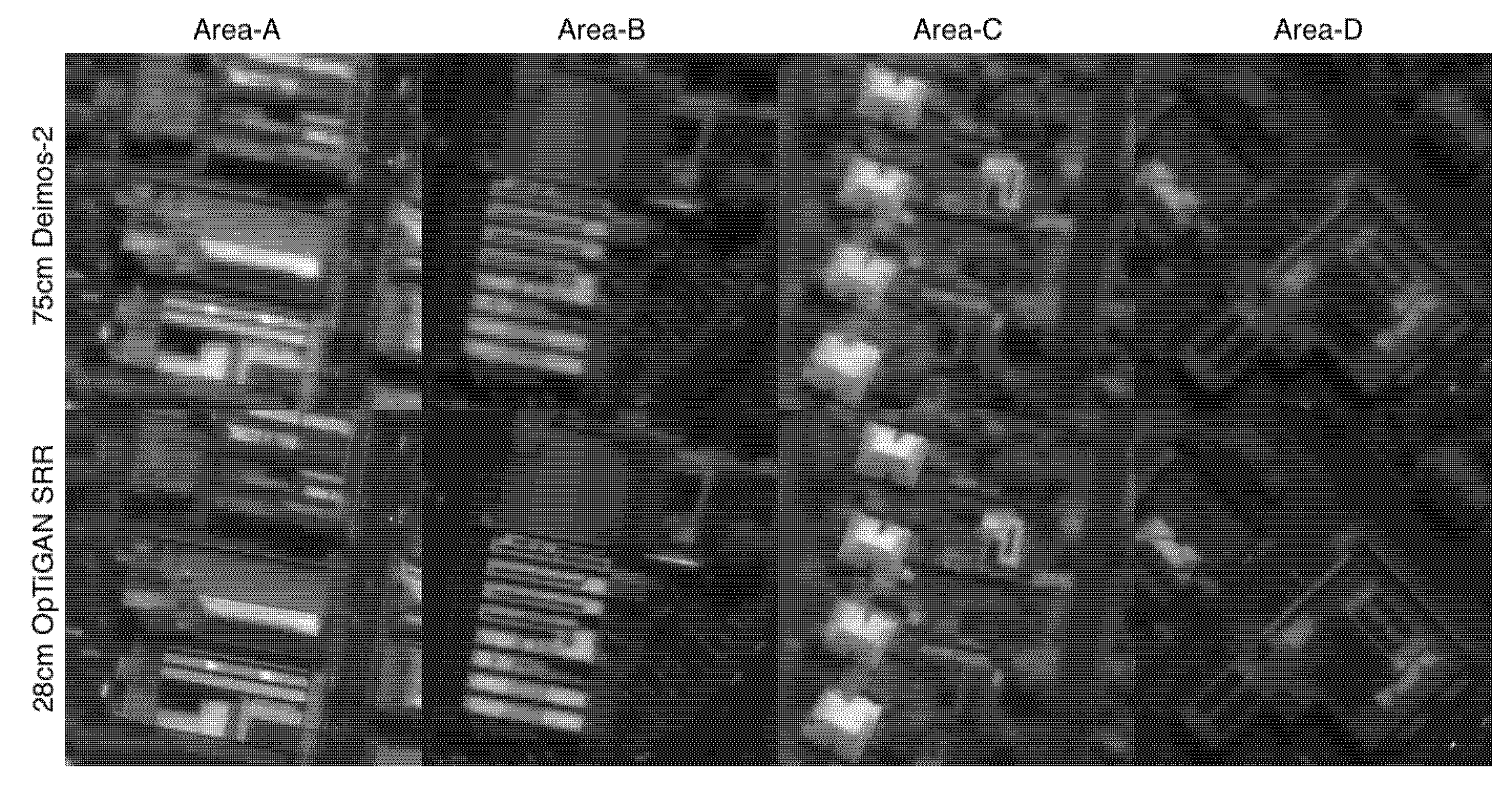
For the Deimos-2 experiments, we used one input for the SRGAN, ESRGAN and MARSGAN SRR processing and three repeat-pass inputs for OFTV and OpTiGAN SRR processing. Four cropped areas (A–D) covering the different artificial targets at the Baotou Geocal site are shown in Figure 8 for comparison with the SRR results and the original input Deimos-2 image.

Area A showed the overall area of the bar-pattern targets that ranged from 25 m × 5 m to 2 m × 0.1 m. We can observe that all five SRR techniques were able to bring out the correct outlines for the 10 m × 2 m bars; however, the ESRGAN results displayed some artefacts (incorrect shape) and the OFTV results were slightly smoother than the others. For the smaller 5 m × 1 m bars, only ESRGAN, MARSGAN and OpTiGAN results showed some reasonable restoration, but with added noise. Some details could be seen for the 4.5 m × 0.9 m bars with MARSGAN and OpTiGAN, but with too much noise.

Area B showed the centre of the knife-edge target. We can observe that the SRGAN, ESRGAN and OFTV results were quite blurry at the centre and edges. In addition, ESRGAN tended to produce some artificial textures that made the edges even more blurry. MARSGAN showed sharper edges in comparison to SRGAN, ESRGAN and OFTV. OpTiGAN showed further improvement on top of MARSGAN.

Area C showed a zoom-in view of the smaller 10 m × 2 m and 5 m × 1 m bar-pattern targets. We could clearly observe the noise in SRGAN and ESRGAN for the 10 m × 2 m bars. The OFTV result was blurry, but without any artefact. MARSGAN and OpTiGAN had the best (and similar) restoration for the 10 m × 2 m bars. For the 5 m × 1 m bars, only OpTiGAN produced reasonable restoration.

Area D showed a fan-shaped target. We can observe that all five SRR results showed good restoration of the target at mid-to-long radius. At the centre of the fan-shaped target, the SRGAN and OFTV results were blurry and the ESRGAN, MARSGAN and OpTiGAN results showed different levels of artefact.

In

Table 5. BRISQUE and PIQE assessment of the Deimos-2 image and its SRR results at Baotou Geocal site.

	Deimos-2	SRGAN	ESRGAN	MARSGAN	OFTV	OpTiGAN
BRISQUE	44.775	47.1044	44.0127	39.5407	44.4973	39.3605
PIQE	75.446	65.798	22.4199	25.2007	24.1284	25.0122

, we show the BRISQUE and PIQE image quality scores (0–100, lower score represents better quality) that were measured with the full-image (see Supplementary Materials for the full-image) at the Baotou Geocal site. We can observe improvements in terms of image quality from all five SRR techniques. MARSGAN and OpTiGAN received the best overall score for the Deimos-2 results.

In Figure 9, we present a quantitative assessment achieved via the Imatest^® slanted-edge measurements for the knife-edge target at the Baotou Geocal site. There were three automatically detected edges and their associated 20–80% profile rise analysis are shown, for each of the input Deimos-2 image, SRGAN SRR result, ESRGAN SRR result, MARSGAN SRR result, OFTV SRR result and OpTiGAN SRR result. The total pixel counts for the 20–80% profile rise of each slanted edge is summarised in

Table 6. Summary of slanted-edge measurement, as shown in Figure 9, for total pixel counts for the 20–80% rise of the edge profile and indicated effective resolution enhancement factor comparing to the input Deimos-2 image (upscaled by a factor of 4 for comparison).

	Deimos-2	SRGAN	ESRGAN	MARSGAN	OFTV	OpTiGAN
Edge-1 pixel counts	8.7 pixels	8.98 pixels	8.61 pixels	6.43 pixels	8.7 pixels	2.87 pixels
Edge-1 enhancement factor	-	<1 times	>1 times	1.35 times	1 times	3.03 times
Edge-2 pixel counts	8.06 pixels	8.21 pixels	7.83 pixels	7.54 pixels	8.49 pixels	3.19 pixels
Edge-2 enhancement factor	-	<1 times	>1 times	1.07 times	<1 times	2.53 times
Edge-3 pixel counts	7.9 pixels	6.85 pixels	7.13 pixels	4.98 pixels	7.62 pixels	3.15 pixels
Edge-3 enhancement factor	-	1.15 times	>1 times	1.59 times	>1 times	2.51 times
Average enhancement factor	-	~1 times	~1 times	~1.34 times	~1 times	~2.69 times

. We divided the total pixel counts of the input Deimos-2 image (upscaled by a factor of 4 for comparison) with the total pixel counts of the SRR results to get the effective resolution enhancement factor for each of the measured edge. The three measurements were then averaged to get the final effective resolution enhancement factor, as shown in the last row of Table 6. For the Deimos-2 experiments, we can observe that the effective resolution enhancements were generally not good with SRGAN, ESRGAN and OFTV; however, with OpTiGAN, we still obtained a factor of 2.96 times improvement.

The other quantitative assessment of image effective resolution was achieved via visual checking of the smallest resolvable bar targets for each of the SRR results. The results are summarised in

Table 7. Summary of the effective resolution derived from Figure 9 and Table 6, the smallest resolvable bar pattern targets observed from the Deimos-2 image and each of the SRR results, in comparison with Figure 5, as well as the number of input images used and computing time for the Baotou Geocal site.

	Deimos-2	SRGAN	ESRGAN	MARSGAN	OFTV	OpTiGAN
Image size	284 × 284 pixels	1136 × 1136 pixels
Spatial resolution	75 cm/pixel	18.75 cm/pixel
Effective resolution	Assuming 75 cm/pixel	75 cm/pixel	75 cm/pixel	56 cm/pixel	75 cm/pixel	28 cm/pixel
Smallest resolvable bar (recognisable)	2 m	2 m	1 m	1 m	2 m	1 m
Smallest resolvable bar (with good visual quality)	3 m	2 m	3 m	2 m	2 m	2 m
Number of LR input used	-	1	1	1	3	3
Computing time	-	<1 s	<1 s	<1 s	~6 min	~6 min

. We can observe, from Table 7, that even the effective resolutions for edges were generally not good for SRGAN, ESRGAN and OFTV, as shown in Table 6. The results still showed reasonable restorations for the bar targets. We can see, from Table 7, that, with a 75 cm/pixel resolution Deimos-2 image, we can resolve 2 m/3 m bar targets and, with a 28 cm/pixel OpTiGAN SRR, we can resolve 1 m/2 m bar targets.

3.4. Demonstration and Assessments of SkySat Results

For the SkySat experiments, we used one input for the SRGAN, ESRGAN and MARSGAN SRR processing and five continuous video frames for the OFTV and OpTiGAN SRR processing. Four cropped areas (A–D) covering the different artificial targets available at the Baotou Geocal site are shown in Figure 10 for comparison with the SRR results and the original input SkySat video frames.

Area A showed the overall area of the bar-pattern targets that ranged from 25 m × 5 m to 2 m × 0.1 m. We can observe that SRGAN, MARSGAN, OFTV and OpTiGAN were able to bring out the correct outlines of the 10 m × 2 m bars. The ESRGAN result showed some high-frequency textures and also showed some reconstruction of the 5 m × 1 m bars; however, its result was very noisy. OFTV was blurry, but with the least artefact. The MARSGAN and OpTiGAN results showed the best restoration with little noise and artefact, for the bar-pattern targets, and, especially, for bringing out the 5 m × 1 m bars. A few textures have been revealed for the 4.5 m × 0.9 m bars from OpTiGAN, but no individual 4.5 m × 0.9 m bar has been resolved from any SRR result.

Area B showed the centre of the knife-edge target. We can observe artefacts from SRGAN, noise from ESRGAN, blurring effects from MARSGAN and OFTV. In terms of edge sharpness for this area, SRGAN and OpTiGAN results were the best, but OpTiGAN had significantly less artefact and noise compared to SRGAN.

Area C showed a zoom-in view of the smaller 10 m × 2 m and 5 m × 1 m bar-pattern targets. For the smaller 5 m × 1 m bars, the MARSGAN and OpTiGAN results showed some good restoration, but both with artefacts and noise.

Area D showed the fan-shaped target. The ESRGAN result showed the best restoration at the centre, but it was also the noisiest. SRGAN displayed artefacts towards the centre. MARSGAN and OpTiGAN showed the best restoration for mid-to-long radiuses.

Finally, we give BRISQUE and PIQE image quality scores (0–100, lower scores represent better quality) in

Table 8. BRISQUE and PIQE assessment of the SkySat video frame (reference frame) and its SRR results at Baotou Geocal site.

	SkySat	SRGAN	ESRGAN	MARSGAN	OFTV	OpTiGAN
BRISQUE	43.4582	39.0124	28.4039	34.0242	40.0536	36.0347
PIQE	69.0228	37.6772	35.2918	28.8104	33.6981	29.4606

. We can observe significant improvements in terms of image quality from all five SRR results. ESRGAN, MARSGAN and OpTiGAN demonstrated the best overall score for the SkySat experiments.

In Figure 11, we present the Imatest^® slanted-edge measurements for the knife-edge target. There were three automatically detected edges and their associated 20–80% profile rise analysis are shown, for each of the input SkySat video frames, SRGAN, ESRGAN, MARSGAN, OFTV and OpTiGAN SRR results. The total pixel counts for the 20–80% profile rise of each slanted edge is summarised in

Table 9. Summary of slanted-edge measurement as shown in Figure 11, for total pixel counts for the 20–80% rise of the edge profile and indicated effective resolution enhancement factor comparing to the input SkySat video frame (upscaled by a factor of 4 for comparison).

	SkySat	SRGAN	ESRGAN	MARSGAN	OFTV	OpTiGAN
Edge-1 pixel counts	7.69 pixels	6.09 pixels	3.55 pixels	3.15 pixels	5.27 pixels	1.76 pixels
Edge-1 enhancement factor	-	1.26 times	2.17 times	2.44 times	1.46 times	4.37 times
Edge-2 pixel counts	7.80 pixels	6.37 pixels	6.02 pixels	5.36 pixels	6.95 pixels	1.82 pixels
Edge-2 enhancement factor	-	1.22 times	1.30 times	1.46 times	1.12 times	4.29 times
Edge-3 pixel counts	5.45 pixels	3.57 pixels	3.35 pixels	3.10 pixels	5.72 pixels	1.72 pixels
Edge-3 enhancement factor	-	1.53 times	1.63 times	1.76 times	<1 times	3.17 times
Average enhancement factor	-	~1.34 times	1.7 times	~1.89 times	~1.19 times	~3.94 times

. We divided the total pixel counts of the input SkySat video frame (upscaled by a factor of 4 for comparison) with the total pixel counts of the SRR results to get an indicative effective resolution enhancement factor for each of the measured edge. The three measurements were then averaged to get the final effective resolution enhancement factor, as shown in the last row of Table 9. For the SkySat experiments, we can only observe marginal effective resolution enhancements for SRGAN, ESRGAN, MARSGAN and OFTV; however, with OpTiGAN, the effective resolution enhancement factor was much higher, at 3.94 times.

The smallest resolvable bar targets from the original SkySat video frame and its SRR results are summarised in

Table 10. Summary of the effective resolution derived from Figure 11 and Table 9, the smallest resolvable bar pattern targets observed from the SkySat image and each of the SRR results, in comparison to Figure 5, as well as the number of input images used and computing time for the Baotou Geocal site.

	SkySat	SRGAN	ESRGAN	MARSGAN	OFTV	OpTiGAN
Image size	183 × 183 pixels	732 × 732 pixels
Spatial resolution	70 cm/pixel	17.5 cm/pixel
Effective resolution	Assuming 70 cm/pixel	52 cm/pixel	41 cm/pixel	37 cm/pixel	59 cm/pixel	18 cm/pixel
Smallest resolvable bar (recognisable)	2 m	2 m	1 m	1 m	2 m	1 m
Smallest resolvable bar (with good visual quality)	5 m	3 m	5 m	3 m	2 m	2 m
Number of LR input used	-	1	1	1	5	5
Computing time	-	<1 s	<1 s	<1 s	~5 min	~5 min

. With a 70 cm/pixel resolution SkySat video frame, we can resolve 2 m/5 m bar targets. SRGAN brought the 3 m bars to visually good quality. ESRGAN did not improved the quality of the 5 m and 3 m bars, but made the 1 m bar resolvable. MARSGAN improved the quality of the 5 m and 3 m bars and also made the 1 m bar resolvable. OFTV did not make the 1 m bars resolvable, but improved the visual quality for 5 m, 3 m and 2 m bars. Finally, with the 18 cm/pixel OpTiGAN SRR, 1 m bars were resolvable and the qualities for 5 m, 3 m and 2 m bars were all improved.

3.5. OpTiGAN Results Demonstration over Different Areas

In this section, we demonstrate further OpTiGAN SRR results for 31 cm WorldView-3 images and 75 cm Deimos-2 PAN band images over different areas. These included small building blocks within the Baotou site, from WorldView-3 (Figure 12), a non-urban area (snow covered) in Greenland, from WorldView-3 (Figure 13), small and flat residential building blocks in Adelaide, from Deimos-2 (Figure 14), and tower buildings, ships and highway roads over Dubai, from Deimos-2 (Figure 15). It should be noted that all OpTiGAN SRR results in this section were produced with four input images from the two datasets (WorldView-3 and Deimos-2) and image IDs of the reference images are given in the figure captions. We can observe from the different examples of urban and non-urban scenes, that OpTiGAN was able to restore structural outlines (e.g., buildings, roads and geological surface features) and small objects (e.g., windows of a building, cars and ships), with much higher edge sharpness and no obvious artefact.

4. Discussion

We can observe from the results, OFTV has played an important role in producing the initial SRR image (intermediate output in the first-stage processing of OpTiGAN) to provide initial controls on potential artefacts and noises, from the follow-on GAN-based refinement process (the second-stage processing in OpTiGAN). Although SRGAN, ESRGAN and MARSGAN alone were able to produce visually pleasing SRR results, due to effects from artefact and noise, we did not observe significant improvement in terms of resolving smaller bar targets, from all three experiments.

In addition, the effective resolutions achieved from SRGAN, ESRGAN and MARSGAN alone, for ultra-high resolution satellite imagery, when a network did not have any prior knowledge of the HR counterpart of the input images (i.e., network had not been trained with any HR truth at such ultra-high spatial resolution), were generally limited, as demonstrated in the slanted-edge measurements. OpTiGAN provides a solution for SRR of ultra-high resolution satellite image sequences or videos.

The proposed multi-image OpTiGAN SRR system benefits from more input images; we based our test on a minimal number of LR inputs and tested its limit for only three LR inputs for the Deimos-2 datasets. We can observe better effective resolution enhancement factors with OpTiGAN using five LR inputs for WorldView-3 and SkySat, in comparison to using three LR inputs for Deimos-2.

However, more LR inputs (or larger input image size) require more computing time. The processing speed of a SRR system that involves MAP approaches is generally not comparable with a deep learning-based inference system. However, with OpTiGAN, as most of the components are portable to GPU, we were able to produce SRR results for small inputs (≤300 × 300 pixels, ≤5 inputs) within a fairly short time (≤10 min). The other downside is that we observed some artefacts, in our experiments from the first stage (OFTV) of the OpTiGAN processing, for using large input LR images (typically for input images >1000 × 2000 pixels). This issue can be fully eliminated by using tiles of smaller input images (≤500 × 500 pixels).

In the future, different optical flow algorithms and/or different SRR networks can be explored to further improve performance of each of the two processing stages of the OpTiGAN system. A multi-scale approach can be explored to replace the current sequential approach, in order to better integrate the traditional MAP solution with the deep learning-based result. Better training of the MARSGAN model is expected in the future, when there are more training images available. In addition, separating the MARSGAN model with respect to different types of targets/surface features (separately trained) may potentially improve the performance. In this case, an automated system to identify such different types of targets and surface features will be helpful both for training (scene classification) and for inferencing (trained model selection).

5. Conclusions

In this paper, we proposed a multi-image SRR system, called OpTiGAN, for continuous ultra-high-resolution satellite image acquisitions or video frames, based on the MAGiGAN SRR system [1]. OpTiGAN is a complementary and lightweight SRR system in comparison to MAGiGAN in terms of using different types of inputs (i.e., non-multi-angle and multi-angle) and takes much shorter computing time. OpTiGAN follows the two-stage processing framework used in MAGiGAN, using a traditional multi-image MAP approach (i.e., OFTV) and a state-of-the-art deep learning-based approach (i.e., MARSGAN). In this way, we produced the best effective resolution improvement with the least artefact.

We have shown the optimal performance of OpTiGAN, in comparison to the two popular single-image deep learning-based SRR techniques (i.e., SRGAN and ESRGAN), as well as the two processing stages of OpTiGAN alone (i.e., OFTV and MARSGAN), for processing of different geocal/MTF datasets that have the highest spatial resolutions. Generally speaking, there is barely any SRR technique that has demonstrated with ultra-high resolution satellite images (30–80 cm/pixel), due to the lack of HR counterpart for training. We have demonstrated resolution improvement for such datasets, via the proposed two-stage SRR processing, that combines the advantages from a classic MAP technique and a new deep learning-based single-image SRR technique.

In this work, we have provided quantitative assessments and qualitative evaluations for SRR results on the artificial optical targets available at the Baotou Geocal site. We demonstrated 3.69 times effective resolution enhancement with the proposed OpTiGAN SRR system for the 31 cm WorldView-3 images, 2.69 times effective resolution enhancement for the 75 cm Deimos-2 images and 3.94 times effective resolution enhancement for the 70 cm SkySat video frames.

References

1. Tao, Y.; Muller, J.P. Super-resolution restoration of MISR images using the UCL MAGiGAN system. Remote Sens. 2019, 11, 52. [Google Scholar] [CrossRef] [Green Version]
2. Shin, D.; Muller, J.-P. Progressively weighted affine adaptive correlation matching for quasi-dense 3D reconstruction. Pattern Recognit. 2012, 45, 3795–3809. [Google Scholar] [CrossRef]
3. Tao, Y.; Muller, J.P. A novel method for surface exploration: Super-resolution restoration of Mars repeat-pass orbital imagery. Planet. Space Sci. 2016, 121, 103–114. [Google Scholar] [CrossRef] [Green Version]
4. Ledig, C.; Theis, L.; Huszár, F.; Caballero, J.; Cunningham, A.; Acosta, A.; Aitken, A.P.; Tejani, A.; Totz, J.; Wang, Z.; et al. Photo-Realistic Single Image Super-Resolution Using a Generative Adversarial Network. CVPR 2017, 2, 4. [Google Scholar]
5. Farneback, G. Two-frame motion estimation based on polynomial expansion. Lect. Notes Comput. Sci. 2003, 2749, 363–370. [Google Scholar]
6. Farsiu, S.; Robinson, D.; Elad, M.; Milanfar, P. Fast and robust multi-frame super-resolution. IEEE Trans. Image Process. 2004, 13, 1327–1344. [Google Scholar] [CrossRef] [PubMed]
7. Cullingworth, C.; Muller, J.-P. Contemporaneous Monitoring of the Whole Dynamic Earth System from Space, Part I: System Simulation Study Using GEO and Molniya Orbits. Remote Sens. 2021, 13, 878. [Google Scholar] [CrossRef]
8. Peleg, S.; Keren, D.; Schweitzer, L. Improving image resolution using subpixel motion. Pattern Recognit. Lett. 1987, 5, 223–226. [Google Scholar] [CrossRef]
9. Keren, D.; Peleg, S.; Brada, R. Image sequence enhancement using subpixel displacements. In Proceedings of the IEEE Computer Society Conference on Computer Vision and Pattern Recognition, Ann Arbor, MI, USA, 5–9 June 1988; pp. 742–746. [Google Scholar]
10. Bascle, B.; Blake, A.; Zisserman, A. Motion deblurring and super-resolution from an image sequence. In Proceedings of the 4th European Conference on Computer Vision, Cambridge, UK, 15–18 April 1996; pp. 312–320. [Google Scholar]
11. Cohen, B.; Dinstein, I. Polyphase back-projection filtering for image resolution enhancement. IEE Proc. Vis. Image Signal Process. 2000, 147, 318–322. [Google Scholar] [CrossRef]
12. Zomet, A.; Rav-Acha, A.; Peleg, S. Robust super-resolution. In Proceedings of IEEE International Conference on Computer Vision and Pattern Recognition, Kauai, HI, USA, 8–14 December 2001; pp. 645–650. [Google Scholar]
13. Luttrell, S.P. Bayesian autofocus/super-resolution theory. In Proceedings of IEE Colloquium on Role of Image Processing in Defence and Military Electronics, London, UK, 9 April 1990; pp. 1–6. [Google Scholar]
14. Cheeseman, P.; Kanefsky, B.; Kraft, R.; Stutz, J. Super-Resolved Surface Reconstruction from Multiple Images; Technical Report FIA9412; NASA: Washington, DC, USA, 1994. [Google Scholar]
15. Schultz, R.R.; Stevenson, R.L. A Bayesian Approach to Image Expansion for Improved De_nition. IEEE Trans. Image Process. 1994, 3, 233–242. [Google Scholar] [CrossRef]
16. Pan, M.C.; Lettington, A.H. E_cient method for improving Poisson MAP super-resolution. Electron Lett. 1999, 35, 803–805. [Google Scholar] [CrossRef]
17. Elad, M.; Hel-Or, Y. A fast super-resolution reconstruction algorithm for pure translational motion and common space-invariant blur. IEEE Trans. Image Process. 2001, 10, 1187–1193. [Google Scholar] [CrossRef] [PubMed] [Green Version]
18. Hardie, R.C.; Barnard, K.J.; Armstrong, E.E. Joint MAP registration and high resolution image estimation using a sequence of undersampled images. IEEE Trans. Image Process. 1997, 6, 1621–1633. [Google Scholar] [CrossRef] [PubMed] [Green Version]
19. Schultz, R.R.; Meng, L.; Stevenson, R.L. Subpixel motion estimation for super-resolution image sequence enhancement. J. Vis. Commun. Image Represent. 1998, 9, 38–50. [Google Scholar] [CrossRef]
20. Borman, S.; Stevenson, R.L. Simultaneous multi-frame MAP super-resolution video enhancement using spatio temporal priors. In Proceedings of IEEE International Conference on Image Processing, Kobe, Japan, 24–28 October 1999; pp. 469–473. [Google Scholar]
21. Pickup, L.; Roberts, S.; Zisserman, A. A sampled texture prior for image super-resolution. In Proceeding of the 16th International conference on Advances in Neural Information Processing Systems, Vancouver, Canada, 8–13 December 2003. [Google Scholar]
22. Keller, S.H.; Lauze, F.; Nielsen, M. Video super-resolution using simultaneous motion and intensity calculations. IEEE Trans. Image Process. 2011, 20, 1870–1884. [Google Scholar] [CrossRef] [PubMed]
23. Yuan, Q.; Zhang, L.; Shen, H. Multiframe super-resolution employing a spatially weighted total variation model. IEEE Trans. Circuits Syst. Video Technol. 2012, 22, 379–392. [Google Scholar] [CrossRef]
24. Purkait, P.; Chanda, B. Super resolution image reconstruction through Bregman iteration using morphologic regularization. IEEE Trans. Image Process. 2012, 21, 4029–4039. [Google Scholar] [CrossRef]
25. Zhang, H.; Zhang, Y.; Li, H.; Huang, T.S. Generative Bayesian image super resolution with natural image prior. IEEE Trans. Image Process. 2012, 21, 4054–4067. [Google Scholar] [CrossRef]
26. Dong, C.; Loy, C.C.; He, K.; Tang, X. Learning a deep convolutional network for image super-resolution. In Proceedings of the ECCV 2014, Zurich, Switzerland, 6–12 September 2014; pp. 184–199. [Google Scholar]
27. Kim, J.; Kwon Lee, J.; Mu Lee, K. Accurate image super-resolution using very deep convolutional networks. In Proceedings of the IEEE Conference on Computer Vision and Pattern Recognition, Las Vegas, NV, USA, 26 June–1 July 2016; pp. 1646–1654. [Google Scholar]
28. Dong, C.; Loy, C.C.; Tang, X. Accelerating the super-resolution convolutional neural network. In European Conference on Computer Vision; Springer: Cham, Switzerland, 2016; pp. 391–407. [Google Scholar]
29. Shi, W.; Caballero, J.; Huszár, F.; Totz, J.; Aitken, A.P.; Bishop, R.; Rueckert, D.; Wang, Z. Real-time single image and video super-resolution using an efficient sub-pixel convolutional neural network. In Proceedings of the IEEE Conference on Computer Vision and Pattern Recognition, Las Vegas, NV, USA, 26 June–1 July 2016; pp. 1874–1883. [Google Scholar]
30. Wang, C.; Li, Z.; Shi, J. Lightweight image super-resolution with adaptive weighted learning network. Arxiv Prepr. Arxiv 2019, 1904, 02358. [Google Scholar]
31. Sajjadi, M.S.; Scholkopf, B.; Hirsch, M. EnhanceNet: Single image super-resolution through automated texture synthesis. In Proceedings of the IEEE International Conference on Computer Vision, Venice, Italy, 22–29 October 2017; pp. 4491–4500. [Google Scholar]
32. Wang, X.; Yu, K.; Wu, S.; Gu, J.; Liu, Y.; Dong, C.; Qiao, Y.; Change Loy, C. ESRGAN: Enhanced super-resolution generative adversarial networks. In Proceedings of the European Conference on Computer Vision (ECCV) Workshops, Munich, Germany, 8–14 September 2018. [Google Scholar]
33. Rakotonirina, N.C.; Rasoanaivo, A. ESRGAN+: Further improving enhanced super-resolution generative adversarial network. In Proceedings of the InICASSP 2020–2020 IEEE International Conference on Acoustics, Speech and Signal Processing (ICASSP), Barcelona, Spain, 4 May 2020; pp. 3637–3641. [Google Scholar]
34. Zhang, W.; Liu, Y.; Dong, C.; Qiao, Y. RankSRGAN: Generative adversarial networks with ranker for image super-resolution. In Proceedings of the IEEE/CVF International Conference on Computer Vision, Seoul, Korea, 27 October–2 November 2019; pp. 3096–3105. [Google Scholar]
35. Lim, B.; Son, S.; Kim, H.; Nah, S.; Mu Lee, K. Enhanced deep residual networks for single image super-resolution. In Proceedings of the IEEE Conference on Computer Vision and Pattern Recognition Workshops, Honolulu, HI, USA, 21–26 July 2017; pp. 136–144. [Google Scholar]
36. Yu, J.; Fan, Y.; Yang, J.; Xu, N.; Wang, Z.; Wang, X.; Huang, T. Wide activation for efficient and accurate image super-resolution. Arxiv 2018, arXiv:1808.08718. [Google Scholar]
37. Ahn, N.; Kang, B.; Sohn, K.A. Fast, accurate, and lightweight super-resolution with cascading residual network. In Proceedings of the European Conference on Computer Vision (ECCV), Munich, Germany, 8–14 September 2018; pp. 252–268. [Google Scholar]
38. He, K.; Zhang, X.; Ren, S.; Sun, J. Deep residual learning for image recognition. In Proceedings of the IEEE Conference on Computer Vision and Pattern Recognition, Las Vegas, NV, USA, 26 June–1 July 2016; pp. 770–778. [Google Scholar]
39. Zhang, Y.; Li, K.; Li, K.; Wang, L.; Zhong, B.; Fu, Y. Image super-resolution using very deep residual channel attention networks. In Proceedings of the European Conference on Computer Vision (ECCV), Munich, Germany, 8–14 September 2018; pp. 286–301. [Google Scholar]
40. Kim, J.; Lee, J.K.; Lee, K.M. Deeply-recursive convolutional network for image super-resolution. In Proceedings of the IEEE Conference on Computer Vision and Pattern Recognition, Las Vegas, NV, USA, 26 June–1 July 2016; pp. 1637–1645. [Google Scholar]
41. Tai, Y.; Yang, J.; Liu, X. Image super-resolution via deep recursive residual network. In Proceedings of the IEEE Conference on Computer Vision and Pattern Recognition, Honolulu, HI, USA, 21–26 July 2017; pp. 3147–3155. [Google Scholar]
42. Liu, Z.S.; Wang, L.W.; Li, C.T.; Siu, W.C.; Chan, Y.L. Image super-resolution via attention based back projection networks. In Proceedings of 2019 IEEE/CVF International Conference on Computer Vision Workshop (ICCVW), Seoul, Korea, 27–28 October 2019; pp. 3517–3525. [Google Scholar]
43. Tao, Y.; Conway, S.J.; Muller, J.-P.; Putri, A.R.D.; Thomas, N.; Cremonese, G. Single Image Super-Resolution Restoration of TGO CaSSIS colour images: Demonstration with Perseverance Rover Landing Site and Mars science targets. Remote Sens. 2021, 13, 1777. [Google Scholar] [CrossRef]
44. Tao, Y.; Muller, J.-P. Repeat multiview panchromatic super-resolution restoration using the UCL MAGiGAN system. In Proceedings of the Image and Signal Processing for Remote Sensing XXIV 2018, Berlin, Germany, 10–13 September 2018; Volume 10789. Issue 3. [Google Scholar]
45. Jolicoeur-Martineau, A. The relativistic discriminator: A key element missing from standard GAN. Arxiv 2018, arXiv:1807.00734. [Google Scholar]
46. Mittal, A.; Moorthy, A.K.; Bovik, A.C. No-Reference Image Quality Assessment in the Spatial Domain. IEEE Trans. Image Process. 2012, 21, 4695–4708. [Google Scholar] [CrossRef]
47. Venkatanath, N.; Praneeth, D.; Chandrasekhar, B.M.; Channappayya, S.S.; Medasani, S.S. Blind Image Quality Evaluation Using Perception Based Features. In Proceedings of the 21st National Conference on Communications (NCC) 2015, Mumbai, India, 27 February–1 March 2015. [Google Scholar]
48. Li, C.R.; Tang, L.L.; Ma, L.L.; Zhou, Y.S.; Gao, C.X.; Wang, N.; Li, X.H.; Wang, X.H.; Zhu, X.H. Comprehensive calibration and validation site for information remote sensing. Int. Arch. Photogramm. Remote Sens. Spat. Inf. Sci. 2015, 40, 1233. [Google Scholar] [CrossRef] [Green Version]
49. Zhou, Y.; Li, C.; Tang, L.; Ma, L.; Wang, Q.; Liu, Q. A permanent bar pattern distributed target for microwave image resolution analysis. IEEE Geosci. Remote Sens. Lett. 2016, 14, 164–168. [Google Scholar] [CrossRef]
Figure 1. Example of the original 31 cm WorldView-3 image and the 9 cm OpTiGAN SRR result (WorldView-3 image, Maxar, 2020. Data provided by the European Space Agency).
Remotesensing 13 02269 g001
Figure 2. Simplified flow diagram of the MAGiGAN SRR system described in [1]. N.B.: darker coloured boxes represent the inputs and outputs.
Remotesensing 13 02269 g002
Figure 3. Flow diagram of the proposed OpTiGAN SRR system showing the same details as the flow diagram of MAGiGAN, in Figure 2, with changed components indicated in yellow. N.B.: darker coloured boxes represent the inputs and outputs.
Remotesensing 13 02269 g003
Figure 4. Simplified network architecture of the MARSGAN model [43].
Remotesensing 13 02269 g004
Figure 6. WorldView-3® SRR results, from SRGAN, ESRGAN, MARSGAN, OFTV and OpTiGAN, of four cropped areas on the bar-pattern targets, the knife-edge target and the fan-shaped target, at the Baotou Geocal site. Please refer to the Supplementary Materials for full-resolution images at larger size. WorldView-3 image courtesy of Maxar 2020. Data provided by the European Space Agency.
Remotesensing 13 02269 g006
Figure 7. Imatest® slanted-edge profile measurements for the knife-edge target at the Baotou Geocal site, showing 3 automatically detected edges for each of the input WorldView-3 image (upscaled by a factor of 4 for comparison), SRGAN SRR result, ESRGAN SRR result, MARSGAN SRR result, OFTV SRR result and OpTiGAN SRR result. For each slanted edge measurement, there is a plot, showing a profile line crossing the detected edge. Imatest® measured the total pixel count of a 20–80% profile rise. For texts inside the plots, please refer to the original full-resolution figure in Supplementary Materials. WorldView-3 image courtesy of Maxar 2020. Data provided by the European Space Agency.
Remotesensing 13 02269 g007
Figure 8. Deimos-2 SRR results, from SRGAN, ESRGAN, MARSGAN, OFTV and OpTiGAN, of four cropped areas on the bar-pattern target, knife-edge target and fan-shaped target, at the Baotou Geocal site. Please refer to the Supplementary Materials for full-resolution images with larger size. Deimos-2 image courtesy of Deimos Imaging, S.L. 2021.
Remotesensing 13 02269 g008
Figure 9. Imatest® slanted-edge profile measurements for the knife-edge target at the Baotou Geocal site, showing 3 automatically detected edges for each of the input Deimos-2 image (upscaled by a factor of 4 for comparison), SRGAN SRR result, ESRGAN SRR result, MARSGAN SRR result, OFTV SRR result and OpTiGAN SRR result. For each slanted edge measurement, there is a plot, showing a profile line crossing the detected edge. Imatest® measured the total pixel count of a 20–80% profile rise. For text inside the plots, please refer to the original full-resolution figure in Supplementary Materials. Deimos-2 image courtesy of Deimos Imaging, S.L. 2021.
Remotesensing 13 02269 g009
Figure 10. SkySat SRR results, from SRGAN, ESRGAN, MARSGAN, OFTV and OpTiGAN, of four cropped areas on the bar-pattern target, knife-edge target and fan-shaped target, at the Baotou Geocal site. Please refer to the Supplementary Materials for full-resolution images with larger size. SkySat image: Skysat L1A imagery provided by Planet Labs, Inc.
Remotesensing 13 02269 g010
Figure 11. Imatest® slanted-edge profile measurements for the knife-edge target at the Baotou Geocal site, showing 3 automatically detected edges for each of the input SkySat video frames (upscaled by a factor of 4 for comparison), SRGAN SRR result, ESRGAN SRR result, MARSGAN SRR result, OFTV SRR result and OpTiGAN SRR result. For each slanted edge measurement, there is a plot, showing a profile line crossing the detected edge. Imatest® measured the total pixel count of a 20–80% profile rise. For texts inside the plots, please refer to the original full-resolution figure in the Supplementary Materials. SkySat image: Skysat L1A imagery provided by Planet Labs, Inc.
Remotesensing 13 02269 g011
Figure 12. Examples of the 31 cm/pixel WorldView-3 image (18AUG18040034-P2AS-012860253020_01_P006) crops and the corresponding OpTiGAN SRR results showing small buildings over the Baotou site. All sub-figures have a size of 27 m by 27 m. WorldView-3 image courtesy of Maxar 2020. Data provided by the European Space Agency.
Remotesensing 13 02269 g012
Figure 13. Examples of the 31 cm/pixel WorldView-3 image (20MAY16150148-P2AS-012860253010_01_P002) crops and the corresponding OpTiGAN SRR results showing snow surface features over a Greenland site. All sub-figures have a size of 27 m by 27 m. WorldView-3 image courtesy of Maxar 2020. Data provided by the European Space Agency.
Remotesensing 13 02269 g013
Figure 14. Examples of the 75 cm/pixel Deimos-2 image (DE2_PAN_L1B_000000_20180506T021306_20180506T021310) crops and the corresponding OpTiGAN SRR results showing residential building blocks over the Adelaide site. All sub-figures have a size of 87.5 m by 87.5 m. Deimos-2 image courtesy of Deimos Imaging, S.L. 2021.
Remotesensing 13 02269 g014
Figure 15. Examples of the 75 cm/pixel Deimos-2 image (DE2_PAN_L1B_000000_20180624T071049_20180624T071052) crops and the corresponding OpTiGAN SRR results showing building towers, ships and roads over the Dubai site. All sub-figures have a size of 87.5 m by 87.5 m. Deimos-2 image courtesy of Deimos Imaging, S.L. 2021.
Remotesensing 13 02269 g015