Abstract
Collapsed buildings are usually linked with the highest number of human casualties reported after a natural disaster; therefore, quickly finding collapsed buildings can expedite rescue operations and save human lives. Recently, many researchers and agencies have tried to integrate satellite imagery into rapid response. The U.S. Defense Innovation Unit Experimental (DIUx) and National Geospatial Intelligence Agency (NGA) have recently released a ready-to-use dataset known as xView that contains thousands of labeled VHR RGB satellite imagery scenes with 30-cm spatial and 8-bit radiometric resolutions, respectively. Two of the labeled classes represent demolished buildings with 1067 instances and intact buildings with more than 300,000 instances, and both classes are associated with building footprints. In this study, we are using the xView imagery, with building labels (demolished and intact) to create a deep learning framework for classifying buildings as demolished or intact after a natural hazard event. We have used a modified U-Net style fully convolutional neural network (CNN). The results show that the proposed framework has 78% and 95% sensitivity in detecting the demolished and intact buildings, respectively, within the xView dataset. We have also tested the transferability and performance of the trained network on an independent dataset from the 19 September 2017 M 7.1 Pueblo earthquake in central Mexico using Google Earth imagery. To this end, we tested the network on 97 buildings including 10 demolished ones by feeding imagery and building footprints into the trained algorithm. The sensitivity for intact and demolished buildings was 89% and 60%, respectively.
1. Introduction
When a natural hazard event hits a populated area, rapid assessment of infrastructure damage is essential for assessing resource needs and initiating a rapid and appropriate response. As most human fatalities occur in collapsed buildings, immediate detection and mapping of damaged buildings can expedite rescue operations and loss estimations to save lives. Currently, post-disaster damage assessment largely relies on field survey and reconnaissance reports [1]. Recently, satellite and aerial imagery have been used to map damage to the built environment after natural hazards [2]. Today, there are many satellites orbiting the Earth and capturing images from the Earth’s surface with very high resolution (VHR) (spatial resolution less than 1 m) and increasing temporal resolution. The advantage of these VHR imageries compared with more traditional satellite imageries is that more details can be observed, and smaller objects can be distinguished. Commercial satellite imagery companies sometimes provide imagery with only three Red, Green, and Blue (RGB) spectral channels in the aftermath of a natural disaster, while satellites usually capture imagery with a higher number of spectral bands. Commercially available satellites can capture the same spot on Earth multiple times a day (Planet Company has such satellites), a week (Maxar Company, formerly known as Digital Globe, has such satellites), or a month. The Maxar Company often provides the processed ready-to-use RGB imagery quickly to the community after rapid-onset events like natural disasters, including creating archives such as Maxar’s Open Data Portal. In addition, Maxar contributed processed ready-to-use RGB imagery to the U.S. Defense Innovation Unit Experimental (DIUx) and National Geospatial Intelligence Agency (NGA) xView dataset [3] that contains thousands of labeled VHR satellite imagery scenes. Due to this increased availability of processed ready-to-use VHR satellite imagery, many investigators and agencies have become interested in using satellite imagery to map damage to the built environment after a natural hazard event. Moreover, aerial imagery can be captured using drones or aircraft after a natural hazard event with even higher spatial resolution (less than 10 cm) than satellite imagery. However, aerial imagery usually needs permission from local authorities.
Many researchers have investigated statistical methods for the detection of post-event damages to the built environment using satellite imagery. Comparing pre- and post-event images and detecting damages by looking at changes in pixel values has been a popular method for a long time [4,5,6,7]; however, it can only be applied to one single event, needs extensive human supervision, and needs extensive pre-processing if the pre-event imagery from the same sensor is not available. Several studies have been conducted on land cover segmentation and building damage classification on satellite imagery using conventional machine learning algorithms such as the artificial neural network (ANN), support vector machine (SVM), and random forest techniques [8,9,10]. For example, [11] used object-based image analysis (OBIA) in combination with SVM on Quickbird satellite imagery to perform damage detection in Port-au-Prince after the 2010 Haiti earthquake. In another effort, [10] created an ANN with spectral, textural, and structural input parameters to detect damage to buildings due to the 2010 Haiti earthquake; they used the UNITAR dataset, which included footprints of the damaged buildings in the affected area to validate their results. Both of these studies only focused on damage detection for a single event using data for that event and did not test the portability of the method. In order to develop a method that can be trained ahead of time and applied rapidly in the aftermath of a natural disaster, we need to test the transferability of a detection algorithm on new datasets.
In order to build a damage detection algorithm that can be applied on new events, we looked into Convolutional Neural Networks (CNNs), which are popular in many computer vision tasks, such as image classification, object detection, and image segmentation [12]. Compared with the traditional ML methods mentioned above, CNNs simulate the human visual system to perform a hierarchical abstraction on the image to detect the desired objects. CNNs automatically extract features and classify by using convolutional, subsampling, and fully connected layers [12]. As the feature extraction patterns are learned directly from the image, CNNs have better generalization ability and precision over traditional ML methods. Recently, Fully Convolutional Networks (FCNs) have become more attractive due to their better computational efficiency and lower memory costs [12]. Instead of utilizing small patches and fully connected layers to predict the class of a pixel, FCNs utilize sequential convolutional, subsampling, and up-sampling operations to generate pixel-to-pixel translations between the input image and output map. As no patches or fully connected layers are required, FCNs considerably reduce memory costs and the number of parameters, which significantly improves processing efficiency [11]. Due to FCNs’ high efficiency, numerous investigations have used them recently on different topics, including detecting damage to the built environment [13,14,15,16,17,18]. Note that one of the important factors in all Convolutional Networks for having a high accuracy and successful generalization is to prepare large and diverse training data. If we only use data from a certain event, then we may overfit our network by just showing samples from the single event to it and, therefore, it will not able to make accurate predictions for new events (unseen data). Moreover, a low number of training samples would result in low accuracy when the network is tested with new samples. In order to have a reliable deep learning framework for detecting demolished buildings after a natural hazard event, we need to have a high quality and diverse dataset. While there are various sources of imagery data to evaluate the aftermath of natural disasters, they are not usually in an easily accessed format [19]. To overcome this issue, the xView dataset has been developed by the Defense Innovation Unit Experimental (DIUx) and NGA for a broad range of research in computer vision and object detection [3]. xView is one of the largest publicly available datasets of labeled satellite imagery. It has thousands of satellite images containing different labeled objects on the ground, including intact and demolished buildings. The buildings are identified using labels. All images in the xView dataset are captured by the Maxar Company’s Worldview 3 sensor and have a spatial resolution of 30 cm and a radiometric resolution of 8 bits, are provided in RGB (Red, Green, and Blue spectral bands) channels, and are ready to use by the community (level 2B; no further processing needed). The images have therefore been corrected for atmospheric effects, orthorectified, and pansharpened. The combination of the labeled xView dataset and recent advances in the computer vision community provides an excellent opportunity to develop an automated framework to detect demolished buildings after a natural disaster.
In this paper, our goal was to train a fully Convolutional Neural Network (CNN), called U-Net [20] (details in the following sections), to label demolished and intact buildings after a natural hazard event using VHR RGB satellite imagery such as that provided by Maxar’s Open Data program and Google Earth base maps. To train the U-Net CNN, we used the xView imagery and the demolished and intact building labels. We evaluated the performance of the network first on test data from xView and then on a new event that was not included in xView: the 2017 Puebla, Mexico, earthquake. For the 2017 Puebla, Mexico, earthquake, we used satellite RGB imagery from the Google Earth base map (captured by the Maxar Company Worldview 2 sensor) with the same radiometric resolution but a lower spatial resolution (50 cm) than xView. The Google Earth images have the same level of processing and are ready to use. Using the 2017 Puebla, Mexico, earthquake imagery, we digitized and labeled 97 building footprints, including 10 demolished ones, as our ground truth labels.
2. Dataset: xView Satellite Imagery
One of the motivations for this research was the free availability of thousands of chipped satellite imagery scenes provided recently by the Defense Innovation Unit Experimental (DIUx) and National Geospatial Intelligence Agency (NGA), known as xView [3]. xView is a collection of thousands of chipped satellite imagery scenes and corresponding label information for many objects within the scene. The motivation for the dataset is to stimulate the creation of sophisticated, novel, and robust models and algorithms that can detect different objects on the ground level. The xView dataset is large (e.g., the imagery covers more than 1400 square kilometers) and has a very high spatial resolution (30-cm resolution). All the images have been corrected for atmospheric effects, orthorectified, and pansharpened. xView contains more than 2 million labeled instances across 60 object categories. This diversity in object classes makes xView suitable for applied research across a variety of fields, including disaster response. In this work, we focused on two specific classes related to disaster response which are associated with building footprints: demolished and intact buildings, with 1067 and ~300,000 of labeled instances, respectively, within the whole imagery dataset across the world to account for geographic diversity. For our purposes, we consider the labels to be demolished and intact buildings. Each geographic location has its own specific natural and artificial features such as physical differences (forest, coastal, desert) and constructional differences (layout of houses, cities, roads); this geographical diversity will increase the perspective of objects within a class [3]. Note that the xView dataset is provided as hundreds of large chipped satellite imagery scenes (around 5000 scenes) with different objects labeled on them. We selected only the scenes which contain at least one demolished building label and then trained the network based only on the demolished building and intact building labels, which are associated with building footprints within those selected imagery scenes. This left 153 image chips, with 1067 demolished buildings and 18251 intact buildings. All the imagery scenes within xView are from Maxar (formerly Digital Globe) and were captured by the Worldview 3 sensor, thus eliminating the spectral bias across images and minimizing the variation of spectral information between the same objects in different images. xView provides the satellite imagery only in three visible bands (Red, Green, Blue). The xView labeling process has been carried out by humans and with extensive care and multiple quality standards [3]. Label quality has been controlled in three stages: (1) labeler, (2) supervisor, and (3) an expert. For more details about the labeling process, please refer to the xView dataset manual provided by [3]. Figure 1 shows an example of how the xView provides demolished and intact building labels, shown as red and blue boxes, respectively. As visible in this example of an imagery scene, not all buildings are labeled. In this work, we used the building footprints to mask the image so that only the labeled buildings were used in the training and testing.
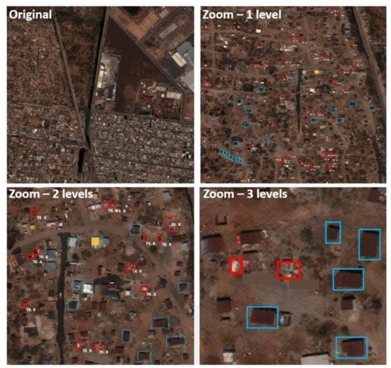
Figure 1.
One satellite imagery scene from the xView dataset with demolished buildings shown in red boxes and intact buildings in blue boxes. The image scene is shown at three zoom levels.
3. Network Architecture
U-Net was originally proposed by [20] to solve biomedical imaging problems; however, soon after, it became popular in other fields of the computer vision research communities. The U-Net style CNN architecture consists of contracting and expanding paths. High-resolution features in the contracting path are concatenated with up-sampled versions of global low-resolution features in the expanding path to help the network learn both local and global information. Figure 2 shows the architecture of a U-Net style convolutional network.
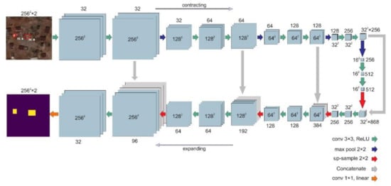
Figure 2.
The U-Net style convolutional neural networks used in this study. The input patch size to the network in our study is 256 by 256 pixels. As shown in this example, the building footprints are used to mask the image. The purple portion of the image is not used in training the algorithm.
As compared with the original U-Net architecture, we also used two regularizing operations to improve the training process: (1) batch normalization [21] and (2) dropout [22]. The batch normalization (BN) operation is used to reduce the amount by which the hidden unit values shift around. The BN operation normalizes the output of a previous activation layer by subtracting the batch mean and dividing by the batch standard deviation. In this research, we used BN at every convolutional layer. Dropout, like BN, is a regularization method that ignores some neurons during the training phase randomly; therefore, the ignored neurons will not be considered in the forward or backward pass. In a fully connected layer and during the training phase, neurons develop interdependency between each other that could result in over-fitting of the training data. By using the dropout operation and ignoring some of the trained neurons, we try to prevent the network from over-fitting.
4. Methodology and Accuracy Measurement
As discussed earlier, there were 1067 demolished and 18,251 intact building labels, respectively in the 153 selected xView imagery scenes in our study dataset. Because this is a heavily unbalanced dataset, we randomly selected 1067 intact building labels out of 18,251 across all 153 imagery scenes to balance the dataset. This made sure that the network statistics were not biased toward the intact building class due to the larger sample size. A biased network can assign higher probabilities to the majority class to avoid greater penalty (higher loss). However, in reality, data often exhibit class imbalance, where some classes are represented by a large number of pixels but other classes by a few (e.g., more intact buildings versus demolished buildings) [23]. Note that the size of each of the xView original satellite imagery scenes is about 3000 by 3000 pixels (each pixel has a resolution of 30 cm). For this study, we generated 256 by 256 pixel-sized patches out of these scenes that contained demolished and/or intact building label(s) because more graphical memory and computational power were required for the network to store the features needed to learn the pattern of demolished and intact building footprints with an increase in input image size. We explain how these patches are generated in the data augmentation section.
4.1. Data Augmentation
Another step taken before feeding the network with training data was data augmentation. CNNs usually require a large quantity of data to achieve convergence of the training process, prevent over-fitting, and minimize the loss. To this end, it is a common practice in the computer vision community to increase the number of samples synthetically or to augment the original data. Augmentation is a process in which the network is fed the same ground truth label(s) multiple times, while, each time, the orientation, position, or size of the label(s) is different. In this study, as the original number of demolished building labels was low (1067), we used the shifting technique to augment the dataset. Shifting is similar to a sliding kernel over the original imagery scene that creates multiple 256 by 256 pixels patches, which contain the whole ground truth label(s) within them. Figure 3 shows an example in which one intact building label is fed to the network in nine different orientations. Note that we have augmented the intact building labels only after randomly selecting 1067 labels out of 18,251 of the original number within the 153 xView selected scenes to maintain an unbiased approach toward both demolished and intact building labels. Out of the 153 original satellite imagery scenes, 130 were randomly selected and used for training (containing 902 intact and 823 demolished labels) and the remaining 23 for testing (containing 166 intact and 244 demolished labels). Using the shifting technique, we generated 256 by 256 pixels patches out of the original scenes that contained demolished and/or intact building label(s) within them. At the end, we had 10,000 256 by 256 pixels patches for training that overall have 13,099 and 12,168 demolished and intact building labels, respectively. Each patch could include multiple labels from both classes or at least one label from one class. The same augmentation procedure was performed for the 23 testing satellite imagery scenes, and 2000 patches were generated with 1243 and 1103 labels for the demolished and intact building classes, respectively. Figure 4 shows two examples of patches used to train the network.
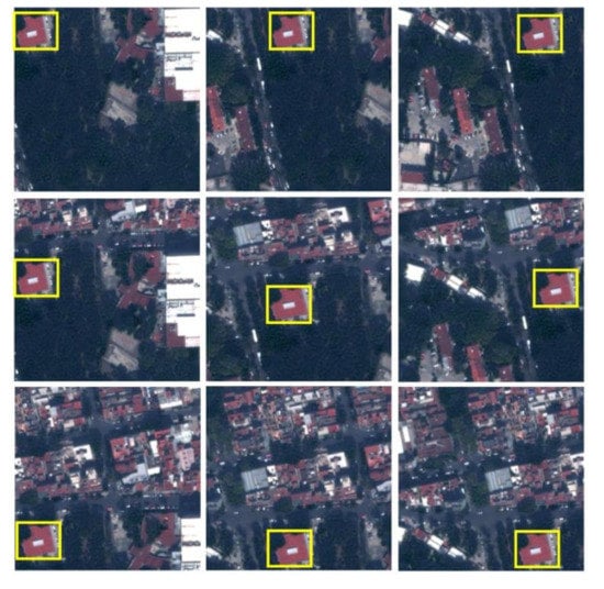
Figure 3.
An example of data augmentation (shifting): an intact building label is fed to the network in nine different orientations.
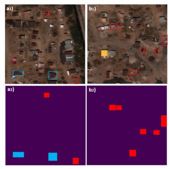
Figure 4.
Two examples of input pairs (top row image and bottom row ground truth labels) to the network: (a1) A patch includes two labels for each of the classes; (a2) Ground truth mask for a1 patch; (b1) A patch includes only six labels of the demolished building class; (b2) Ground truth mask for b1 patch.
Each single patch was normalized by its maximum RGB value before it was fed into the network to increase the learning speed. The network was trained with 16 patches at each input batch and for 1000 epochs. The learning rate was set to 0.0001 to ensure that the network optimizer would not be trapped in local minima. The stochastic gradient descent (SGD) optimization algorithm was used to minimize the loss function. SGD is one of the dominant techniques in CNN optimization [24] and has proven to be effective in optimization of large-scale deep learning models [25]. Categorical cross-entropy loss (Softmax loss) was used as the loss function to output the probability map over the two classes.
For measuring the accuracy of the network, after the training data were used to train the network, a confusion matrix was generated against the validation data. A confusion matrix is a table that summarizes the performance of a classifier by presenting the number of ground truth pixels for each class and how they have been classified by the classifier. There are several important accuracy measurements that can be calculated from a confusion matrix; amongst them are: (1) overall accuracy, (2) producer’s accuracy (sensitivity), and (3) user’s accuracy. Overall accuracy is calculated as the ratio of the total number of correctly classified pixels to the total number of the test pixels. The overall accuracy is an average value for the whole classification method and does not reveal the performance of the method for each class. Producer’s (sensitivity) and user’s accuracies are defined for each of the classes. The producer’s accuracy is also common, as classifier sensitivity corresponds to errors of omission (exclusion or false negative rate) and shows how many of the pixels on the classified map are labeled correctly for a given class in the reference data. Producer’s accuracy is calculated as:
where PC is the number of pixels correctly identified in the reference plot and PA is the number of pixels actually in that reference class.
User’s accuracy corresponds to the errors of commission (inclusion or false positive rate) and shows how many pixels on the classified map are correctly classified. User’s accuracy is calculated as:
where PG is the number of pixels correctly identified in a given map and PCL is the number of pixels claimed to be in that map class. We also calculated and reported the specificity defined as TN / TN + FP, where TP, FP, and FN are the true positive, false positive, and false negative rates, respectively. User’s accuracy, producer’s accuracy (sensitivity), and specificity were calculated for intact and demolished buildings.
All pre-processing, training, and testing tasks were performed on Tufts University’s High Performance Cluster configured with 128 GB of RAM, 8 cores of 2.6 GHz CPUs, and an NVIDIA Tesla P100 GPU. All tasks were coded in Python language using various libraries including Numpy, Shapely, Keras, and Tensorflow.
5. Results
The primary goal of the trained U-Net network was to identify demolished and intact buildings from post-event VHR RGB imagery (such as that available through Maxar’s Open Data Program or with imagery provided as Google Earth base maps) paired with building footprints. In other words, the trained U-Net network will assign a probability value for each class in each pixel; the class with higher probability will be considered as the network prediction. As a common practice, if both class probabilities for a given pixel are less than 50%, then that pixel will be classified as neither (missed). Using the xView dataset as described above, we trained a U-Net network to detect intact and demolished buildings. The optimum network is called UXV_B, where U stands for the U-Net algorithm, XV stands for the training data, and B stands for building. The UXV_B network’s performance was evaluated on testing (unseen) data from the xView dataset. Figure 5 illustrates the network predictions of pixel probability for one patch, where Figure 5a is the post-event imagery, Figure 5b is the ground truth labels, Figure 5c is the prediction for intact building class and Figure 5d is the network predictions for the demolished building class. In Figure 5c,d, yellow indicates higher probability for the class. As can be seen in Figure 5c (the network’s attempt to detect intact buildings), the network predicts the pixels within the intact buildings’ footprint with higher probability compared with the pixels within the demolished buildings’ footprint. In Figure 5d (the network’s attempt to detect demolished buildings), the network gives higher probability to pixels within the demolished buildings’ footprint compared with the intact buildings’ footprint. Note that the network assigns probabilities to pixels within the buildings’ footprint, rather than to the entire tile. In Figure 5d, there are some pixels within the intact building boxes mistakenly classified as demolished building labels, although with a lower probability than pixels within the demolished building boxes. If we evaluate the network performance at the pixel level, the sensitivity of the model to detect demolished building is 60.3%. This low value partly relates to the fact that class probabilities are not consistent across a building footprint and accuracy diminishes near the edges of the building footprint. This edge effect can influence the spectral and textural information extraction process by the network, which is supposed to only learn the demolished and intact building pixels and not the ones around them.
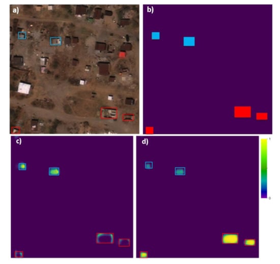
Figure 5.
An example of the network’s probability prediction: Boxes in red and blue are demolished and intact building labels, respectively. (a) Post-event imagery (input to the network). (b) Input label mask (ground truth); blue shows intact building labels and red shows demolished building labels. (c) Network predictions for the intact building class. (d) Network predictions for the demolished building class.
6. Discussion
To alleviate the abovementioned issue and improve the final network performance, we considered the overall performance of the network based on the individual building labels rather than by pixel. In other words, instead of evaluating the performance of the network for each pixel, we used the pixel-based class probabilities to assign a label to each building and then evaluated the network’s performance by building. To this end, the building is assigned a label based on which class had the majority of labeled pixels with a predicted probability of higher than 50% and only if the majority pixels covered at least 30% of the building footprint area; otherwise, the label is assigned neither of the classes. Figure 6 shows the network prediction for one demolished building label. If we measure the accuracy of the network for this footprint pixel-wise, then only 57% of the pixels are correctly classified (network sensitivity is 57%), but if we consider the accuracy of the building (label-wise) and according to our earlier definition, then the label is correctly classified as one instance of the demolished building class.
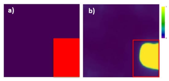
Figure 6.
Redefining the accuracy measurement of the network: (a) ground truth of a demolished building; (b) network probability prediction. Pixel-wise, only 57% are correctly classified, but label-wise and according to our definition, the network has correctly classified this as one instance of a demolished building label (one true positive).
After redefining the accuracy measurement, the confusion matrix for the network prediction was generated and is presented in Table 1. According to the matrix and Equations (1) and (2), the user’s and producer’s (sensitivity) accuracies for the demolished building class are 97% and 76%, respectively. The user’s and producer’s accuracies for the intact building class are 79% and 96%. Out of 1243 demolished building labels, 281 are misclassified as intact buildings, while out of 1103 labels for intact building labels, only 33 are misclassified as demolished buildings. Overall, the UXV_B network can predict the correct label with 85% accuracy. Table 2 presents the producer’s accuracy (sensitivity) and specificity for both the demolished and intact building classes. As can be seen, the producer’s accuracy (sensitivity) of detecting the intact building class is much higher than that of detecting the demolished building class (96% vs. 76%); however, its specificity for the demolished building class is higher than that of the intact building class (97% vs. 77%). Specificity (precision) is the network’s capability to truly detect negative labels (how many negative selected instances are truly negative).

Table 1.
Confusion matrix against the labels in xView testing dataset using the 30% areal percentage threshold.
Table 2.
Network’s producer’s accuracy (sensitivity) and specificity to input classes using the 30% areal percentage threshold.
We evaluated the areal percentage threshold effect for assigning a class label to a building footprint with 20%, 30%, 40%, and 70% values (we used 30%, as described earlier) and the results are summarized in Table 3. Lower threshold values (e.g., 20%) slightly increases the sensitivity, as fewer missed labels will remain. On the other hand, higher thresholds decrease the sensitivity as the number of missing labels increases. Choosing a proper threshold depends on the application of the network and the quality of the labeling and/or training process. Higher thresholds imply that the labeling and/or training process is more accurate, and one would expect the network to predict more pixels within the labels. Users can select the threshold based on their needs. As presented in Table 3, the differences between accuracies when using 20%, 30%, and 40% thresholds are not considerable. However, if we use 70% as a very conservative threshold, then the sensitivity falls down to 44% and 77% for the demolished and intact classes, respectively, as the number of missing labels increases. According to the 70% threshold results, accurate detection of demolished buildings is significantly reduced (more so than intact buildings). This is an indication that intact buildings can be detected across a greater area of the building footprint, while demolished buildings may only be detected over a smaller portion of the building footprint. This could lead to differences in areal thresholds for the two building classes. Note that increasing the areal percentage threshold would only increase the number of missing labels in each class and consequently, decrease the model’s sensitivity. In other words, playing with this threshold will not change the model’s prediction from demolished to intact and vice versa.
Table 3.
Effect of areal percentage thresholds on the network’s accuracy.
6.1. Evaluating the Trained Network’s Performance on Detecting the Demolished Buildings after the 2017 M 7.1 Puebla Earthquake in Mexico
To evaluate the trained UXVB network, we tested the transferability of the UXVB network on a new set of images acquired through the Google Earth base map of historical imagery after the 19 September 2017 M 7.1 Pueblo earthquake in Mexico. The imagery was originally acquired by WorldView-2 and has been processed to the level 2B (provided as pansharpened, georeferenced, and orthorectified). The Google Earth base map is in RGB format and has 50 cm spatial resolution, which is lower than that of the xView dataset (30 cm spatial resolution) but both have same 8-bit radiometric resolution. Note that even though the spatial resolution is lower, CNNs are known to have reasonable performance when facing data with different resolutions or sizes [26]. Nineteen buildings collapsed due to the earthquake in Mexico City, although the damage was more widespread in other central parts of Mexico. As the weather was partly cloudy in the aftermath of the event in Mexico City, only 10 of the collapsed buildings were visible in the immediate semi-hazy post-event satellite imagery captured on 19 September 2017 (same day). As the cleanup process was relatively quick in the city, collapsed buildings’ debris was mostly removed in the post-event imagery available on 20 October 2017 (1 month after the event). After locating the 10 demolished buildings through the Google Earth base map and generating 256 by 256 pixel patches, 87 intact buildings were also selected manually in the resulting imagery patches used for this case study. Note that we generated the building footprints (labels) for this set of 97 buildings visually and used them to test the trained UXVB network. Figure 7 shows two sets out of nine patches with the network’s prediction of demolished and intact buildings (the remaining seven patches can be found in Appendix A). Note that we used the building footprints to mask the image; therefore, the network only evaluated the image within the building footprints in the imagery patches. After we implemented the 30% thresholds discussed earlier, each building was labeled as demolished or intact. In Figure 7a1–c1, the network correctly predicted all intact and demolished buildings (11 intact and one demolished); in Figure 7a2–c2, the network correctly predicted six out of eight intact buildings and one out of two demolished buildings. The building footprints with false predictions are shown with a red cross behind them in Figure 7b2,c2. The confusion matrix of the model predictions for all 97 instances is presented in Table 4. The network has correctly labeled six demolished buildings while missing the remaining four (60% producer’s accuracy or sensitivity). For the intact buildings, the network’s performance is higher, with correct labels for 78 out of 87 instances (89% producer’s accuracy or sensitivity). Note that, as presented in Table 4, the network confused two instances of intact buildings with demolished buildings, while no instances of demolished buildings were confused with intact buildings (97% and 100% specificity for the demolished and intact building labels, respectively). It is interesting to note that the demolished buildings were either correctly classified or not classified. None of them was mis-classified as intact.
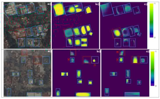
Figure 7.
Network prediction after the 2017 M 7.1 Pueblo earthquake in Mexico: (a1,2) satellite imagery tiles labeled as demolished (red) and intact (blue) buildings; (b1,2) network’s prediction of intact building instances; (c1,2) network’s prediction of demolished building instances. Satellite images from Google Earth; all rights reserved. Red x indicates footprints mis-classified or missed by the network.
Table 4.
Confusion matrix against the labels for the 2017 Pueblo, Mexico, earthquake testing dataset.
One reason for having lower sensitivity values on the 2017 Mexico earthquake dataset in comparison with the xView testing set could be due to the lower spatial resolution of the Google Earth base map. Moreover, the semi-cloudy weather (low sunlight) in the aftermath of the Mexico earthquake and the haziness of several patches could have affected the network’s capability in assigning the correct class to the labels. However, in Figure 7 and the patches in Appendix A, some patterns in how the network performs can be observed; for example, the network can generally predict footprints with bright colors with high probability as intact labels. In Figure 7a2, the top demolished footprint is hazy and therefore the network could not predict it correctly. Moreover, in the same figure, two intact buildings at the top are close to two collapsed buildings and therefore, because of the heavy debris within the building footprints, the network confused the intact buildings with demolished ones. Furthermore, as can be seen in Figure 7 and Appendix A, in many footprints, the network’s prediction does not cover the whole area. In other words, the accuracy measurements depend on the value of the areal percentage threshold. If we decrease the 30% threshold, we will have higher sensitivity.
7. Conclusions
Rapid response to natural disasters is of critical importance, as it can save human lives and help with recovery. Demolished or collapsed buildings after such hazards can cause high numbers of casualties. In this research, a deep learning framework based on CNN architecture and the xView dataset was proposed to detect demolished buildings in VHR optical RGB imagery after natural hazard events. Using 1067 demolished building labels and 1067 intact building labels from the xView dataset to create a balanced training dataset, we trained a network. Using the shifting augmentation technique, we trained a U-Net style convolutional neural network (CNN) with roughly 10,000 patches including around 13,000 labels each of the demolished and intact building classes. While the initial function of the network was set to detect demolished pixels, we defined a threshold that if 30% of pixels within a label were classified correctly and they had the majority of counted pixels between the two classes, then the network had successfully predicted the correct class for that label. The results show that the proposed network’s producer’s accuracy or sensitivity to detect the demolished and intact building classes was 76% and 95%, respectively.
We tested the network performance using a set of imagery after the 19 September 2017 Puebla, Mexico, earthquake from a Google Earth base map with the same radiometric resolution as xView but a lower spatial resolution (50 cm vs. 30 cm from xView) including 10 and 87 instances of demolished and intact buildings, respectively. The network’s producer’s accuracy or sensitivity for the demolished and intact building labels was 60% and 89%, respectively (lower than its performance on the xView dataset), likely due to the reduced resolution (50 cm versus 30 cm), cloudy weather, and haziness of the imagery patches. That being said, none of the demolished buildings was misclassified as an intact building. The proposed network could be implemented in rapid response with the acquisition of Worldview 2 or Worldview3 RGB imagery in the immediate aftermath of a natural disaster. Note that this framework has been constructed and trained with very high-resolution (30 cm) optical satellite imagery from Maxar Company captured after disastrous events (xView dataset). The UXV_Bs-trained network can be implemented on future earthquakes to generate a map of demolished buildings. Depending on the computational power and size of the affected area, this process would only take minutes to accomplish.
Author Contributions
Conceptualization, M.K.; Data curation, V.R.; Formal analysis, V.R.; Funding acquisition, L.G.B., M.K. and B.M.; Investigation, V.R. and L.G.B.; Methodology, V.R. and M.K.; Project administration, L.G.B.; Resources, L.G.B.; Supervision, L.G.B. and B.M.; Writing—original draft, V.R.; Writing—review & editing, B.M. All authors have read and agreed to the published version of the manuscript.
Funding
This material is based upon work supported by the U.S. Geological Survey under Grant Numbers G19AP00056 and G19AP00057.
Institutional Review Board Statement
Not applicable.
Informed Consent Statement
Not applicable.
Data Availability Statement
xVeiw dataset used here is publicly available.
Acknowledgments
This material is based upon work supported by the U.S. Geological Survey under Grant Numbers G19AP00056 and G19AP00057. We gratefully acknowledge this support. The views and conclusions contained in this document are those of the authors and should not be interpreted as representing the opinions or policies of the U.S. Geological Survey. Mention of trade names or commercial products does not constitute their endorsement by the U.S. Geological Survey. The authors would also like to thank the Tufts Technology Service department for providing us with computational resources.
Conflicts of Interest
The authors declare no conflict of interest.
Appendix A
Network prediction probability map on satellite imagery tiles after the 19 September 2017 Pueblo M 7.1 earthquake.


Figure A1.
Network prediction after the 2017 M 7.1 Pueblo earthquake in Mexico on seven different tiles: (a) satellite imagery tiles labeled with demolished (red) and intact (blue) buildings; (b) network’s predictions of intact building instances; (c) network’s prediction of demolished building instances. Satellite images from Google Earth; all rights reserved. Red x indicates footprints mis-classified or missed by the network.


References
- Federal Emergency Management Agency. Damage Assessment Operations Manual; The U.S. Department of Homeland Security: Washington, DC, USA, 2016.
- Duda, K.A.; Jones, B.K. USGS remote sensing coordination for the 2010 Haiti earthquake. Eng. Remote Sens. 2011, 77, 899–907. [Google Scholar] [CrossRef]
- Lam, D.; Richard, K.; Kevin, M.; Samuel, D.; Michael, L.; Matthew, K.; Yaroslav, B.; Brendan, M. xView: Objects in Context in Overhead Imagery. arXiv 2018, arXiv:1802.07856. [Google Scholar]
- Dell’Acqua, F.; Polli, D.A. Post-event only VHR radar satellite data for automated damage assessment. Photogramm. Eng. Remote Sens. 2011, 77, 1037–1043. [Google Scholar] [CrossRef]
- Liu, W.; Yang, J.; Zhao, J.; Yang, L. A Novel Method of Unsupervised Change Detection Using Multi-Temporal PolSAR Images. Remote. Sens. 2017, 9, 1135. [Google Scholar] [CrossRef]
- Byun, Y.; Han, Y.; Chae, T. Image Fusion-Based Change Detection for Flood Extent Extraction Using Bi-Temporal Very High-Resolution Satellite Images. Remote Sens. 2015, 7, 10347–10363. [Google Scholar] [CrossRef]
- Wu, C.; Zhang, F.; Xia, J.; Xu, Y.; Li, G.; Xie, J.; Du, Z.; Liu, R. Building Damage Detection Using U-Net with Attention Mechanism from Pre- and Post-Disaster Remote Sensing Datasets. Remote Sens. 2021, 13, 905. [Google Scholar] [CrossRef]
- Kong, H.; Akakin, H.C.; Sarma, S.E. A generalized Laplacian of Gaussian filter for blob detection and its applications. IEEE Trans. Cybern. 2013, 43, 1719–1733. [Google Scholar] [CrossRef] [PubMed]
- Sun, Z.; Fang, H.; Deng, M.; Chen, A.; Yue, P.; Di, L. Regular shape similarity index: A novel index for accurate extraction of regular objects from remote sensing images. IEEE Trans. Geosci. Remote Sens. 2015, 53, 3737–3748. [Google Scholar] [CrossRef]
- Cooner, A.J.; Shao, Y.; Campbell, J.B. Detection of urban damage using remote sensing and machine learning algorithms: Revisiting the 2010 Haiti earthquake. Remote. Sens. 2016, 8, 868. [Google Scholar] [CrossRef]
- Kaya, G.T.; Ersoy, O.K.; Kamaşak, M.E. Hybrid SVM and SVSA Method for Classification of Remote Sensing Images. In 2010 IEEE International Geoscience and Remote Sensing Symposium; IEEE: Piscataway, NJ, USA, 2010; pp. 2828–2831. [Google Scholar]
- LeCun, Y.; Bengio, Y. Convolutional networks for images, speech, and time series. Handb. Brain Theory Neural. Netw. 1995, 3361, 1995. [Google Scholar]
- Endo, Y.; Adriano, B.; Mas, E.; Koshimura, S. New Insights into Multiclass Damage Classification of Tsunami-Induced Building Damage from SAR Images. Remote Sens. 2018, 10, 2059. [Google Scholar] [CrossRef]
- Moya, L.; Marval Perez, L.R.; Mas, E.; Adriano, B.; Koshimura, S.; Yamazaki, F. Novel Unsupervised Classification of Collapsed Buildings Using Satellite Imagery, Hazard Scenarios and Fragility Functions. Remote Sens. 2018, 10, 296. [Google Scholar] [CrossRef]
- Karimzadeh, S.; Matsuoka, M.; Miyajima, M.; Adriano, B.; Fallahi, A.; Karashi, J. Sequential SAR Coherence Method for the Monitoring of Buildings in Sarpole-Zahab, Iran. Remote Sens. 2018, 10, 1255. [Google Scholar] [CrossRef]
- Tang, Y.; Chen, M.; Lin, Y.; Huang, X.; Huang, K.; He, Y.; Li, L. Vision-Based Three-Dimensional Reconstruction and Monitoring of Large-Scale Steel Tubular Structures. Adv. Civ. Eng. 2020, 2020, 1–17. [Google Scholar]
- Xiu, H.; Shinohara, T.; Matsuoka, M.; Inoguchi, M.; Kawabe, K.; Horie, K. Collapsed Building Detection Using 3D Point Clouds and Deep Learning. Remote Sens. 2020, 12, 4057. [Google Scholar] [CrossRef]
- Adriano, B.; Xia, J.; Baier, G.; Yokoya, N.; Koshimura, S. Multi-Source Data Fusion Based on Ensemble Learning for Rapid Building Damage Mapping during the 2018 Sulawesi Earthquake and Tsunami in Palu, Indonesia. Remote Sens. 2019, 11, 886. [Google Scholar] [CrossRef]
- Chen, S.A.; Escay, A.; Haberland, C.; Schneider, T.; Staneva, V.; Choe, Y. Benchmark dataset for automatic damaged building detection from post-hurricane remotely sensed imagery. arXiv 2018, arXiv:1812.05581. [Google Scholar]
- Ronneberger, O.; Philipp, F.; Thomas, B. U-Net: Convolutional networks for biomedical image segmentation. In International Conference on Medical Image Computing and Computer-Assisted Intervention; Springer: Cham, Switzedland, 2015; pp. 234–241. [Google Scholar]
- Ioffe, S.; Szegedy, C. Batch normalization: Accelerating Deep Network Training by Reducing Internal Covariate Shift. In Proceedings of the 32nd International Conference on International Conference on Machine Learning-Volume, Lille, France, 6–11 July 2015; pp. 448–456. [Google Scholar]
- Srivastava, N.; Hinton, G.; Krizhevsky, A.; Sutskever, I.; Salakhutdinov, R. Dropout: A simple way to prevent neural networks from overfitting. J. Mach. Learn. Res. 2014, 15, 1929–1958. [Google Scholar]
- Oommen, T.; Baise, L.G. Model development and validation for intelligent data collection for lateral spread displacements. J. Comput. Civ. Eng. 2010, 24, 467–477. [Google Scholar] [CrossRef]
- Bottou, L.; Curtis, F.E.; Nocedal, J. Optimization methods for large-scale machine learning. arXiv 2016, arXiv:1606.04838. [Google Scholar] [CrossRef]
- Kingma, D.P.; Ba, J. ADAM: A Method for Stochastic Optimization. In International Conference on Learning Representations; ICLR: San Diego, CA, USA, 2015. [Google Scholar]
- Xu, Y.; Tianjun, X.; Jiaxing, Z.; Kuiyuan, Y.; Zheng, Z. Scale-invariant convolutional neural networks. arXiv 2014, arXiv:1411.6369. [Google Scholar]


Publisher’s Note: MDPI stays neutral with regard to jurisdictional claims in published maps and institutional affiliations. |
© 2021 by the authors. Licensee MDPI, Basel, Switzerland. This article is an open access article distributed under the terms and conditions of the Creative Commons Attribution (CC BY) license (https://creativecommons.org/licenses/by/4.0/).