A Revised Snow Cover Algorithm to Improve Discrimination between Snow and Clouds: A Case Study in Gran Paradiso National Park

Abstract

Snow cover plays an important role in biotic and abiotic environmental processes, as well as human activities, on both regional and global scales. Due to the difficulty of in situ data collection in vast and inaccessible areas, the use of optical satellite imagery represents a useful support for snow cover mapping. At present, several operational snow cover algorithms and products are available. Even though most of them offer an up-to-daily time scale, they do not provide sufficient spatial resolution for studies requiring high spatial detail. By contrast, the Let-It-Snow (LIS) algorithm can produce high-resolution snow cover maps, based on the use of both the normalized-difference snow index (NDSI) and a digital elevation model. The latter is introduced to define a threshold value on the altitude, below which the presence of snow is excluded. In this study, we revised the LIS algorithm by introducing a new parameter, based on a threshold in the shortwave infrared (SWIR) band, and by modifying the overall algorithm workflow, such that the cloud mask selection can be used as an input. The revised algorithm has been applied to a case study in Gran Paradiso National Park. Unlike previous studies, we also compared the performance of both the original and the modified algorithms in the presence of cloud cover, in order to evaluate their effectiveness in discriminating between snow and clouds. Ground data collected by meteorological stations equipped with both snow gauges and solarimeters were used for validation purposes. The changes introduced in the revised algorithm can improve upon the overall classification accuracy obtained by the original LIS algorithm (i.e., up to 89.17 from 80.88%). The producer’s and user’s accuracy values obtained by the modified algorithm (89.12 and 95.03%, respectively) were larger than those obtained by the original algorithm (76.68 and 93.67%, respectively), thus providing a more accurate snow cover map.

1. Introduction

Snow cover plays a fundamental role in mountainous regions, as it is a key factor for different processes, ranging from ecological processes to the energy balance of solar radiation. Moreover, it has a significant influence on hydrological regimes and affects tourism and other human activities related to the presence of snow. For these reasons, the study and monitoring of snow cover has relevant implications in the study of fauna and flora, for risk management, for the study of socio-economic models, and for basin-scale hydrological modelling [1,2,3,4,5,6,7,8,9,10]. Snow cover has also been indicated, by the Global Observing System for Climate (GCOS), as one of the 50 Essential Climate Variables (ECVs), as it is an important variable in monitoring climate change [11]. In situ observations are not sufficient to characterize the properties and distribution of snow, particularly in mountainous areas that are subject to high variability and, often, inaccessibility. However, satellite observations can provide information on the different properties of snow and its distribution with high temporal and spatial continuity [12,13].

Snow detection through the use of optical sensors is related to the reflection/absorption properties of snow. This method suffers from limitations, due to cloud cover and solar illumination, but represents a consolidated field of study, in which detection algorithms have reached maturity [14].

Most optical sensor snow detection algorithms are built using the normalized-difference snow index (NDSI), proposed by Dozier [15], based on the spectral bands of the Landsat Thematic Mapper. This index exploits the spectral signature of snow in order to distinguish it from other land-use classes, which generally have a high reflectance in the visible spectral region, as well as distinguishing it from clouds, which (unlike snow) have a high reflectance in a portion of the shortwave infrared (SWIR) range. Different algorithms have been developed, based on this index, in order to derive many snow parameters, such as the snow cover binary product, the snow depth, the snow water equivalent, or the fractional snow cover [14].

Most of the snow operational products utilize the imagery detected by the Moderate Resolution Imaging Spectroradiometer (MODIS) and the Advanced Very High Resolution Radiometer (AVHRR), which offer a daily temporal resolution, with a spatial resolution ranging between 250 m and 25 km for products at regional to global scale [16,17,18,19]. An algorithm that has been widely affirmed as suitable for use with different optical sensors is SCAmod, proposed by Metsämäki, based “on a semi-empirical model, where the at-satellite observed reflectance is expressed as a function of the fractional snow cover” [19]. This model relies on a forest transmissivity map and, therefore, is particularly suitable for detecting snow in forested areas. At present, this method is implemented for Northern Hemisphere snow extent production in the Copernicus Cryoland project named GlobSnow, which exploits MODIS and Sentinel-3 data to produce daily snow cover extent maps at 500 m resolution. Another publicly available snow cover data set for the European Alps has been offered by EURAC [16]. It provides two different daily products at 250 m resolution, based on MODIS data: EURAC_SNOW, where the algorithm performs the detection of snow cover in open areas based on the NDVI (normalized difference vegetation index), while in forested areas, it is based on a multi-temporal approach; and EURAC_SNOW_CLOUDREMOVAL, a nearly cloud-free version derived from the first product by means of a combination of temporal and spatial filters [20].

The Landsat mission, on the other hand, offers high spatial resolution, but is limited by a review time of 16 days and further diminished by cloud cover, which is very common in temperate mountain areas [21,22,23]. Therefore, it is inadequate for the monitoring of snowpack, which can undergo rapid changes. In a recent study, conducted in the same study area used in this paper, an NDSI-based algorithm for snow detection—namely, the Snow Observations from Space (SOfS) algorithm—was applied to combine cloud-free Landsat images stored in an Open Data Cube into monthly aggregates, which provide the products of the maximum snow cover area for a given month, in the period 1984–2018 [24]. This multi-sensor and multi-temporal approach has proved useful for studying snow trends in time-series in the past; however, it is unsuitable for finer scale monitoring and the study of snow-influenced processes [25]. Conversely, the Sentinel-2 mission provides systematic global acquisitions of high-resolution imagery of the Earth’s surface with a 5-day revisit time at the equator, allowing for outstanding multi-spectral observations and characterization of dynamic surface processes from local to global scales [26]. Gascoin et al. [27] developed a snow cover detection algorithm designed for Sentinel-2 images, based on the NDSI index in combination with the use of a digital elevation model, in order to define a snow altitude threshold, below which the presence of snow is excluded. This algorithm was adopted by the Copernicus Land Monitoring Service and is available at a pan-European scale under the name of High-Resolution Snow & Ice (HR-S & I) products. The validation of this algorithm has given excellent results, despite its tendency to underestimate the snow; however, it has been focused on clear-sky images and the challenge of reducing the misclassification between snow and cloud remains open [27]. Previous studies have also based the validation of snow cover output maps on using reference higher resolution satellite images, field surveys, webcams, or meteorological data, assuming clear-sky conditions [28,29,30,31]. When these conditions are not verified, the main challenge of snow cover mapping through optical imagery is to avoid misclassifications between clouds and snow [14,27,32].

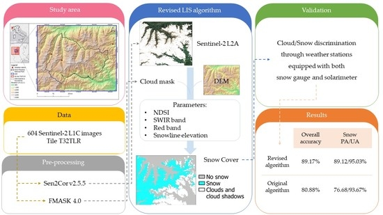
In this study, we revised the Let-It-Snow (LIS) algorithm in order to improve its discrimination between snow and cloud objects. In the pre-processing phase, while LIS adopts the MAJA algorithm [32] for both atmospheric/topographic correction and cloud mask extraction, we introduced the Fmask algorithm [33] and Sen2Cor [34] processor. In the subsequent processing phase, the revised algorithm introduces a new parameter, based on the reflectance in the SWIR, to better discriminate snow from clouds. As a further improvement, the reduction of red-band noise is achieved by smoothing its values through a mean moving window, whereas the original algorithm adopts a band down-sampling technique. Finally, regardless of the amount of snow detected, the proposed algorithm produces an output map; that is, when restrictive threshold values are used for the NDSI, red band, and SWIR band, and a low amount of snow pixels are found (with respect to a defined quantitative threshold), the proposed algorithm provides an output snow cover map, whereas the original LIS algorithm produces no output in this case. This allows, in the case of very high cloud cover, for the detection of snow by applying only the most restrictive thresholds, thus reducing the occurrence of false positives. When the amount of snow pixels is greater than the aforementioned quantitative threshold, the algorithm adopts liberal thresholds for the NDSI, red band, and SWIR band, in order to improve the algorithm’s sensitivity for the detection of additional snow pixels. Another novelty is a contextual analysis, based on the introduction of a procedure that re-assigns clusters smaller than five pixels to the final label, based on neighboring pixels, in the final output.

We applied the revised algorithm to a mountainous study site located in the Italian north-western Alps, that is subject to frequent cloud cover. Finally, we used a new validation approach: investigating the classification accuracy, even in the case of cloudy observations, using ground data collected by a snow gauge and a solarimeter. The findings of the validation phase show that the introduction of the SWIR band can improve snow cover mapping in cloudy images.

The paper is structured as follows: Section 2 describes the area of study, the data used, the revised algorithm, and its publication in an open framework, as well as the validation methodology. Validation was conducted using in situ data collected by a snow gauge and a solarimeter, the results of which are reported in Section 3. Section 4 discusses the improvements and limitations of this study. Finally, Section 5 presents our conclusions and possible future developments.

2. Materials and Methods

2.1. Study Area and Data

2.1.1. Study Area

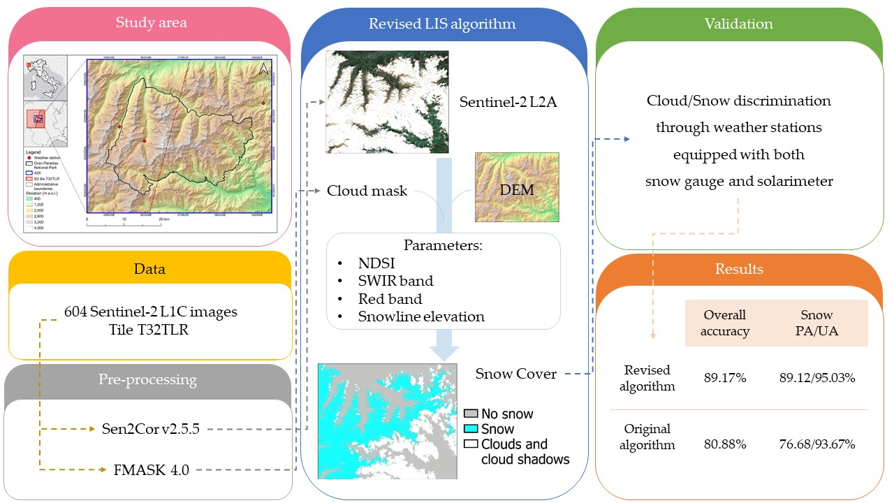
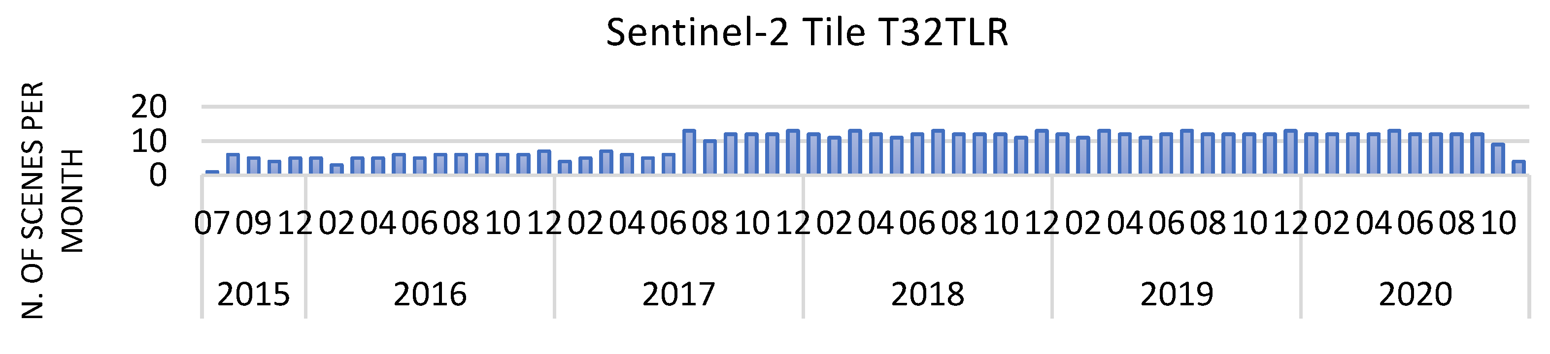
The Area of Interest (AOI) extends over 2065 km² between the Val d’Aosta and Piedmont regions in northern Italy, on the border with France (Figure 1). This area includes the Gran Paradiso massif of the Alpi Graie, and has an elevation ranging from 400 m a.s.l., up to more than 4000 m a.s.l. at the mountain peaks. Glaciers and perennial snows dominate the landscape higher than 3000 m a.s.l. which, as in the rest of the Alpine chain, have been dramatically decreasing due to climate change.

The AOI is centered on Gran Paradiso National Park, the first National Park established in Italy, for the purpose of the conservation of the ibex (Capra ibex), which is also its symbol. The area is characterized by a continental climate, with severe winters lasting from November to April/May. Typically, towards the beginning of the snow season, ephemeral snowfall heralds the arrival of persistent snow, which forms a snowpack that can be greater than 1 m. The snow melting higher than 2000 m a.s.l. occurs, on average, in June. It is not unusual for snowfalls to occur out of season—even in the middle of summer—in which case, however, they have a duration limited to the meteorological event itself. Furthermore, given its topography, the area is often covered by clouds and changes in the weather can occur very quickly.

2.1.2. Data

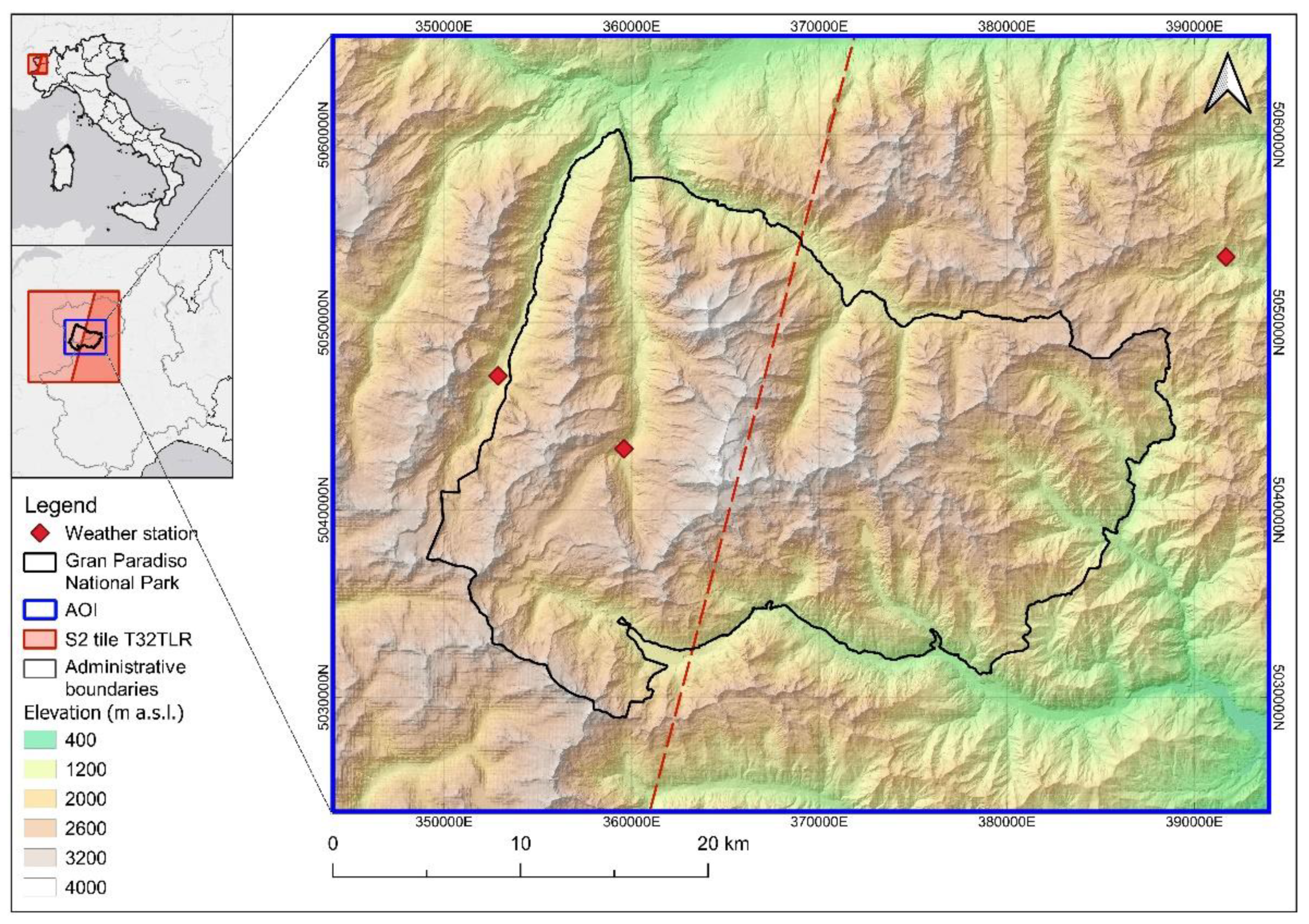
The Sentinel-2 (S2) constellation is made up of twin satellites—S2A and S2B—each of which carries an optical imaging sensor multi-spectral instrument (MSI), which collects reflected radiance in 13 bands (from VIS to SWIR) at different resolutions, ranging from 10 to 60 m [34]. The S2 satellites follow a sun-synchronous orbit at 786 km altitude, with a 290 km swath width. The combination of the two satellites allows for a revisit time of 5 days at the equator and an even shorter time in the mid-latitudes [26]. The S2 images are freely available and are delivered in granules (called tiles) in the UTM/WGS84 projection, each with dimensions of 100 × 100 km². The AOI is entirely covered by the T32TLR tile. Thus, for this study, all the S2 L1C (top-of-atmosphere reflectance) data for the T32TLR tile available from the start of the mission (2015) to the start of the study (12 November 2020) were collected, for a total of 604 images (Figure 2). The initial temporal coverage was 6 scenes per month, which has doubled since July 2017, when the twin satellite S2B became operational.

Given the complex topography of the territory, we decided to use a Digital Elevation Model (DEM) with high spatial resolution. A DEM was therefore developed using the reference system WGS84 UTM 32N at 6.6 m, by combining the following data:

Digital Terrain Model (DTM) at 2 m from the Val d’Aosta Region (DTM 2005/2008 aggregate);

DTM at 5 m from the Piedmont Region (RIPRESA AEREA ICE 2009–2011-DTM 5);

Copernicus DEM at 25 m (EU-DEM v1.1).

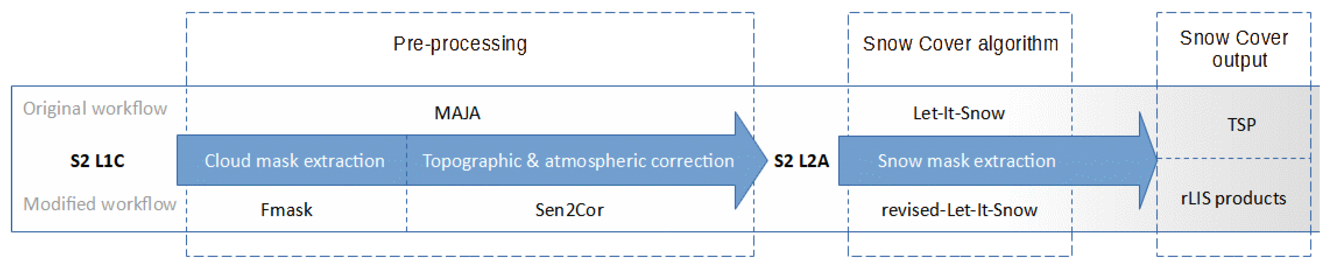
2.2. Workflow and Pre-Processing

The original workflow, proposed by Gascoin et al. [35], carried out S2 L1C pre-processing using the processor MAJA (MACCS-ATCOR Joint Algorithm), a multi-temporal cloud detection and topographic/atmospheric correction software package produced through the joint effort of CNES, CESBIO, and DLR [32]. This workflow has been implemented in the MUSCATE scheduler, which manages the production and distribution of the Theia Snow Products [27], a collection of ready-to-use snow cover products.

In this study, we used a different workflow (Figure 3), which involves the use of two processes: one for cloud cover extraction and one for atmospheric and topographic correction. The cloud cover mask was extracted using Fmask v4.0 [33] (function of mask), software for automated cloud, cloud shadow, snow, and water masking for Landsat 4–8 and Sentinel 2 images. The cloud probability threshold was set to 40%, and the dilation parameters for clouds, cloud shadows, and snow were set to 1, 1, and 0 pixels, respectively.

This choice was driven by the following concerns: previous studies have found that Fmask and MAJA performed similarly in cloud mapping [36,37]; however, MAJA performs at 240 m and, due to processing at a lower resolution, thin clouds with a size of about 100 m may be omitted in the MAJA cloud mask [36]. Moreover, a pre-compiled Windows version of MAJA is not available, while Fmask has been distributed for both Windows and Linux, including standalone versions with or without a graphical user interface (GUI). The S2 L1C images were atmospherically and topographically corrected through Sen2Cor v2.5.5 [34], using the high-resolution DEM described above as auxiliary data, in order to improve the correction performance [38,39], thus obtaining the S2 Level 2A images.

Revised Let-It-Snow Algorithm

To extract the snow cover, the Let-It-Snow (LIS) algorithm, developed by Gascoin et al. [35] and based on the NDSI index [15], was first implemented in the R programming language. We introduced some changes to the LIS algorithm, leading to the proposed algorithm, which was named revised Let-It-Snow (rLIS).

Here, we briefly describe the rLIS algorithm, focusing primarily on its differences from the original algorithm. For more details and a full description of the algorithm, please refer to the specific documentation [35].

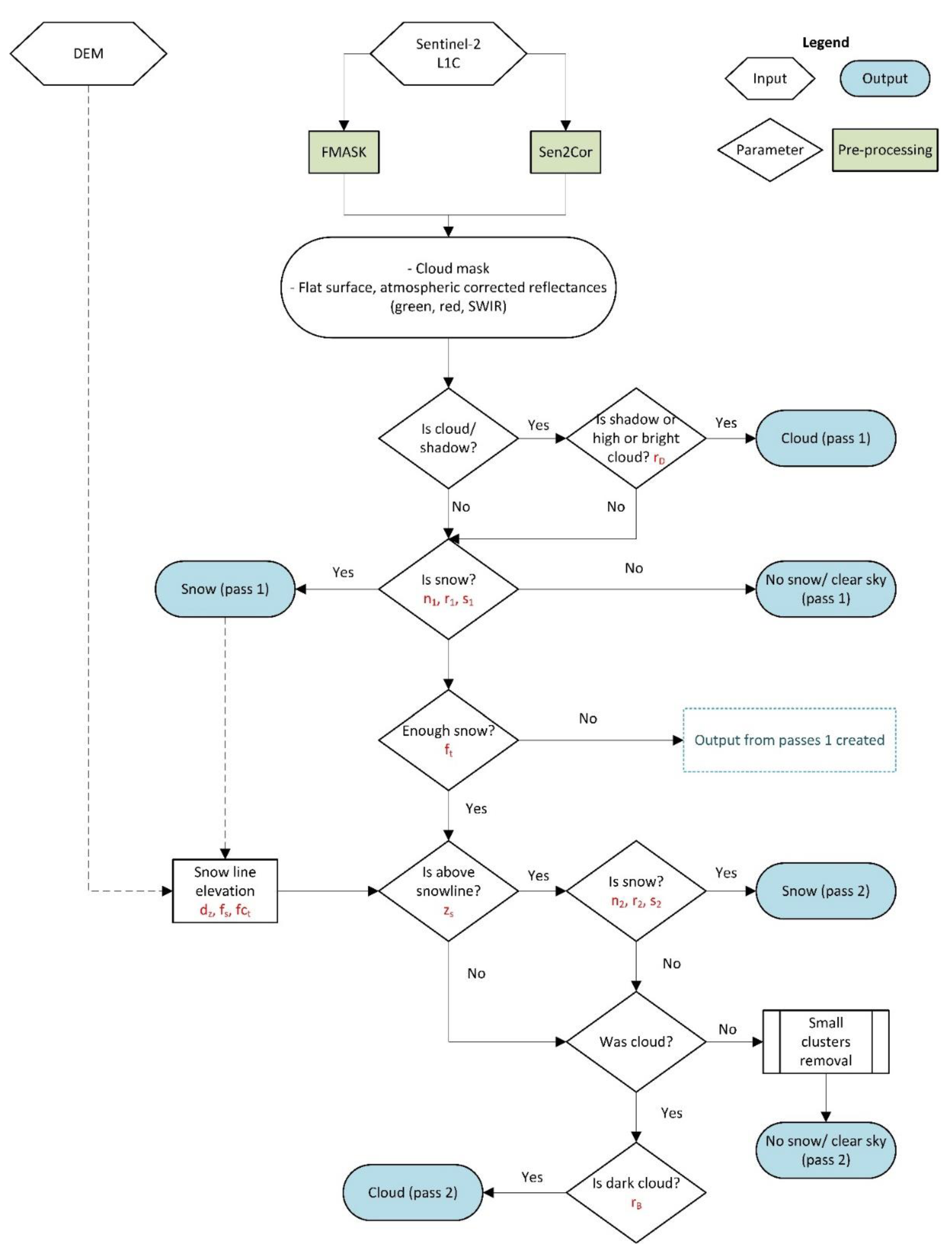
The rLIS algorithm requires three inputs:

An S2 L2A flattened surface bottom-of-atmosphere, in particular the green (band 3); red (band 4), and SWIR (band 11) bands (

Table 1. Spectral bands in flat surface reflectance used by rLIS. The spatial resolution and the band central wavelength are indicated in parentheses.

Bands	Green	Red	SWIR
Sentinel-2	Band 3 (10 m, 0.560 µm)	Band 4 (10 m, 0.665 µm)	Band 11 (20 m, 1.610 µm)

);

The cloud cover mask generated by Fmask [33];

A DEM.

First, the DEM is pre-processed to the same resolution as the S2 L2A 20 m bands. Then, the NDSI is calculated, from the atmospheric and topographically corrected green and SWIR bands at 20 m resolution, as:

$$\mathrm{NDSI} =\frac{\mathrm{green} - \mathrm{SWIR}}{\mathrm{green} + \mathrm{SWIR}}$$

(1)

An important step involves searching for possible snow-covered areas under thin and transparent clouds, defined as “dark clouds”. Hence, in the “cloud pass 1” step, the dark clouds are searched for among all the pixels classified as clouds by Fmask, excluding only the pixels classified a priori as cloud shadows (i.e., 2,

Table 2. Classifications of Fmask and MAJA cloud masks compared [33,36].

Fmask		MAJA
0 1 2 3 4 255	Clear land pixels Clear water pixel Cloud shadows Snow Clouds No data	1 2 4 8 16 32 64 128	Water mask All clouds (subdivided into mono-temporal test, multi-temporal test, high clouds, geometric cloud shadows, radiometric cloud shadow) Snow mask Shadows Topographic shadows Unseen pixels due to topography Sun too low for a correct terrain correction Sun direction tangent to slope

). In the original algorithm, in addition to the cloud shadows, the high-altitude (or cirrus) clouds are excluded a priori from the computation. The “dark clouds” can be identified through use of a threshold, r_D, which is applied to the red band after reducing its noise through an average 3 × 3 moving window filter; in the original LIS process, the smoothing of anomalies is performed by down-sampling the red band by a factor of 12.

Therefore, the pixels flagged as clouds (i.e., 4, Table 2) in the Fmask cloud mask that respond in the red band with a signal greater than r_D (

Table 3. Parameters used in the LIS and rLIS algorithms, readapted from Gascoin et al. [35].

Parameter	Description	Value	rLIS vs. LIS
rf	Rescaling factor to produce the downsampled red band	12 for S2	Deprecated
rD	Maximum value of the downsampled red-band reflectance used to define a dark cloud pixel	0.300	Conserved
n1	Minimum value of the NDSI for the pass 1 snow test	0.400	Conserved
n2	Minimum value of the NDSI for the pass 2 snow test	0.150	Conserved
r1	Minimum value of the red-band reflectance for the pass 1 snow test	0.200	Conserved
r2	Minimum value of the red-band reflectance for the pass 2 snow test	0.040	Conserved
s1	Maximum value of the SWIR-band reflectance for the pass 1 snow test	0.100	Introduced
s2	Maximum value of the SWIR-band reflectance for the pass 2 snow test	0.250	Introduced
dz	Size of elevation band in the DEM used to define zs	100	Conserved
fs	Minimum snow fraction in an elevation band to define zs	0.100	Conserved
fct	Minimum clear pixel fraction (snow and no snow) in an elevation band used to define zs	0.100	Conserved
ft	Minimum snow fraction in the image to activate the pass 2 snow test	0.001	Conserved
rB	Minimum value of the red band reflectance to return a non-snow pixel to the cloud mask	0.100	Conserved

) are temporarily removed from the cloud mask, and are investigated for the possible presence of snow with the rest of the image. These pixels are identified as “dark cloud” pixels. The pixels of the cloud with the red band reflectance lower than r_D are excluded from further investigations.

In the following step, called “snow pass 1” (Figure 4), the snow cover is identified by applying restrictive thresholds in order to minimize false snow detection. Thus, a pixel is classified as snow if the following conditions are fulfilled:

NDSI > n₁;

red band > r₁;

SWIR band < s₁.

As turbid water and cold clouds have NDSI values similar to snow, the red reflectance is used to avoid the misclassification of turbid water surfaces, while the SWIR reflectance is used to avoid cold clouds from being confused with snow. The SWIR band thresholds used in the snow detection steps are a novel feature of rLIS, absent in the original algorithm (Table 3). While the values of classification parameters based on fixed thresholds remained unchanged from those in the original algorithm, for comparison purposes, the new parameter values (i.e., those based on SWIR reflectance) were established using a two-step procedure. First, the distribution of the SWIR spectral response of homogeneous cloud areas was analyzed in order to determine a range of suitable values. Then, these values were tested, using a trial-and-error approach, to refine the selection until the final values were identified.

At this point, if the snow detected in the entire image is greater than the threshold f_t (see Table 3), the algorithm proceeds with the calculation of the snowline elevation; otherwise, it stops. The output is produced by combining “cloud pass 1” and “snow pass 1” (Figure 4). As the AOI is located in an alpine environment, the threshold f_t is almost always overcome, due to the presence of glaciers and perennial snow. When the image is almost or totally cloudy, f_t is not overcome and, therefore, the most restrictive step (i.e., “snow pass 1”) is maintained while the less restrictive one (i.e., “snow pass 2”) is skipped, in order to lower the likelihood of confusion between clouds and snow. In the LIS algorithm, on the other hand, if the total snow threshold f_t is not passed, the algorithm stops, but produces no output.

Thereafter, the snowline elevation is identified by calculating the percentage of snow present for each 100 m (d_z) altitude band, with respect to the percentage of pixels free from clouds (fc_t), thus establishing the altitude limit below which the chance of snow is zero.

The snowline elevation (z_s) is defined as two altitudinal bands below the minimum identified band (d_min) in which the snow that is present is greater than the threshold f_s:

z_s = d_min − 2 · d_z

(2)

Then, the snow detection is performed a second time, using less restrictive thresholds and introducing the previously identified altitude limit, z_s. In this step (called “snow pass 2”), a pixel is classified as snow if it meets the following conditions:

• NDSI > n₂;
• red band > r₂;
• SWIR band < s₂;
• elevation > z_s.

Hence, the previously identified dark cloud pixels that meet the conditions described above are now classified as snow. The remaining dark cloud pixels will return clouds (if they respond in the red band with a reflectance greater than the threshold r_B) or are classified as “No snow,” otherwise. 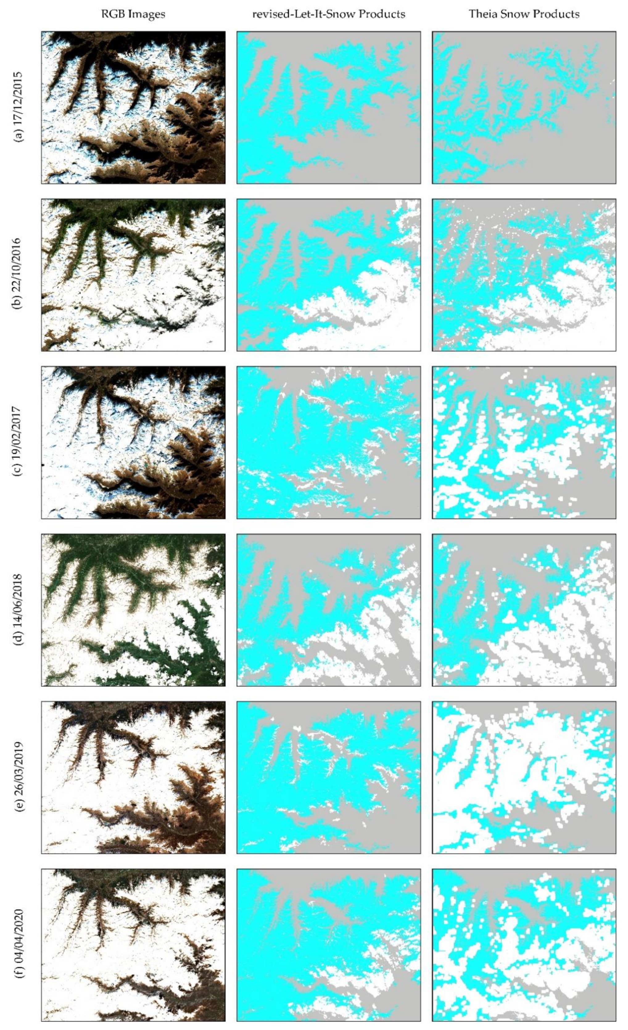The last step is the reclassification of the “No snow” pixel clusters smaller than 5 pixels (equal to 2000 m²), based on the values of the neighboring cells, in order to eliminate any unreliable pixels from the final mask. This passage allows for the elimination of small gaps, which are present mainly in clouds and potentially subject to noisy reflectance and haze. The final output is a 20 m resolution raster mask (Figure 5) following the LIS classification: 0, No snow; 100, Snow; 205, Cloud; 254, No Data.

2.3. Validation

2.3.1. Comparison with In Situ Measurements from Weather Stations

Unlike previous studies based on optical data, which have focused on the ability of algorithms to discriminate only between snow and snow-free areas—and, therefore, excluding cloudy images from validation [18,24,25]—we aimed to evaluate the ability of the proposed algorithm to discriminate snow cover from clouds, as well as from snow-free areas.

In order to achieve this goal, we collected measurements taken from weather stations located within the AOI, equipped with both snow gauges, which measure the amount of solid precipitation, and solarimeters, which measure the flow of solar radiation over a set period of time. These weather stations are owned and managed by the Valle d’Aosta Functional Center (Available online: https://cf.regione.vda.it/home.php (accessed on 12 January 2021)), a service framed within the “Department of Civil Protection and Fire Brigade of the Presidency of the Executive” of the Italian state, which has the main objective of forecasting meteorological phenomena and related effects on the ground. All data collected by the network of meteorological stations are accessible through a dedicated portal (Available online: https://presidi2.regione.vda.it/str_dataview (accessed on 12 January 2021)).

Within the AOI, there were only three stations equipped with both a snow gauge and solarimeter, all located in the Val d’Aosta Region: Rhêmes-Notre-Dame, Chaudanne (5,047,140 N, 352,873 E, 1794 m a.s.l.); Valsavarenche, Pont (5,043,251 N, 359,594 E, 1951 m a.s.l.); and Champorcher, Petit-Mont-Blanc (5,053,489 N, 391,685 E, 1640 m a.s.l.). These weather stations collected continuous punctual measurements, on a half-hourly basis from the snow gauge and averaged over the previous half hour for the solarimeter. We collected these data over the period from 30 July 2015 to 12 November 2020. We then selected the measurements corresponding to the dates and hours that were closest to the acquisition time of the S2 scenes. For example, for the S2 image acquired on 28 June 2020 at 10:25:59 UTC (HH:MM:SS), the validation data compared on the ground were the punctual data acquired at 10:30:00 UTC for the snow gauge, and the averaged data acquired between 10:00:00 and 10:30:00 UTC for the solarimeter. The values from the snow gauge were interpreted as snow in the case that the snow depth >0 cm, and no-snow otherwise. Furthermore, only the measurements with a solarimeter value equal to 30 min (i.e., 30 min out of 30 of sun) or 0 min (i.e., 0 min out of 30 of sun) were considered, in order to discriminate between situations of present or absent cloud cover with certainty.

The classification values of the rLIS algorithm were then extracted from the pixels at which the stations were located. No data values, due to the presence of partial scenes, were excluded. A total of 843 valid observations were found. Of these, in 111 cases the weather stations detected the simultaneous presence of both clouds and snow. These measurements were uncertain for comparison with the classification of the algorithm as, although it was designed with the aim of being able to identify the snow below the most transparent clouds, it is not possible to determine whether the algorithm had correctly identified snow or whether the classification was the result of a misclassification of clouds as snow. Excluding these observations, we took into consideration 732 valid observations for the analysis.

2.3.2. Comparison with Theia Snow Products (TSP)

The Theia Snow Products [27] belong to a collection of ready-to-use snow cover products generated through the original LIS workflow. TSP provide the presence or absence of snow on the land surface every fifth day over selected regions, and is produced and distributed by the Theia Data and Services Centre [40], as 20 m resolution raster and vector files. The workflow for the production of TSP, described in more detail in Section 2.2, carries out the pre-processing of the optical images using the MAJA processor [41], the outputs of which are the inputs to the LIS algorithm.

To evaluate the performance differences between the revised and the original algorithms, all S2 Theia Snow data for tile T32TLR, available from the beginning of the S2 mission up to 12 November 2020, were collected from the Theia Land Data Centre. A total of 484 products were collected. Similarly, the classification values for those pixels in which the weather stations were located were extracted from the TSP. These data were then combined with the in situ measurements from the three weather stations, as described above, into a confusion matrix. The same data set of meteorological observations was also used for the rLIS products, thus creating a third confusion matrix. No data values, due to the presence of partial scenes, were excluded from both data sets. Overall, a total of 591 valid observations were common to rLIS and TSP. Finally, both the revised and original classifiers were compared through contingency tables, for each class and for all classes.

2.3.3. Evaluation Metrics

The data measured by the weather stations were used as a reference data set, in order to build two multiclass confusion matrices, by crossing the reference data set with rLIS and TSP data. The class defined as “Clear/Snow” represents the observations in which the snow gauge has a recorded snow depth > 0 cm and the solarimeter has detected 30 min of sun over 30 min of measurement. The class defined “Clear/Snow-free” constitutes the observations with snow depth = 0 cm and 30 min of sun out of 30, representing the cloud- and snow-free areas. Finally, the “Cloudy/Snow-free” class indicates the observations with snow depth = 0 cm and 0 min of sun over 30 min detected. In order to evaluate the improvement in classification accuracy by the proposed algorithm, the following four parameters were computed: overall accuracy (OA), Kappa coefficient (K), user’s accuracy (UA), and producer’s accuracy (PA) [42].

In addition, McNemar’s chi-squared (χ²) test was used to evaluate the statistical significance of differences between the original and the revised algorithms [43,44,45].

2.4. Publication of Revised Let-It-Snow (rLIS) Algorithm on VLab

The rLIS algorithm, as shown in Figure 4, was published using the Virtual Earth Laboratory (VLab) framework [46], facilitating its exploitability, interoperability between models, and reproducibility of the results.

VLab is a framework that implements all required orchestration functionalities to automate the technical tasks required to execute a model on different computing infrastructures, minimizing the possible interoperability requirements for both model developers and users. Through VLab, modelers can publish models developed in different programming languages and environments. Once a model is available on the VLab, users can request its execution and the framework can trigger its execution on a set of different computing platforms, including cloud platforms such as the European Open Science Cloud, the commercial Amazon Web Services (AWS) cloud, and some Copernicus Data and Information Access Services (DIAS) platforms (e.g., CREODIAS, ONDA, or Sobloo).

Specifically, three modules were published on VLab. Two modules implemented the pre-processing steps, while a third one carried out the snow cover processing: (i) the Fmask module, (ii) the Sen2Cor module, and (iii) the Snow Cover module.

The Fmask module implemented version 4.3 of the Function of Mask algorithm [33], which is devoted to clouds, cloud shadows, snow, and water masking for both Landsat 4–8 and S2 images. The Fmask algorithm was provided by the Global Environmental Remote Sensing Laboratory (GERSL), University of Connecticut, and was developed in MATLAB. The module requires an S2 L1C product as input and optionally parameters, rather than the default ones. The output is a cloud cover mask. The Sen2Cor module was based on the Sen2Cor software [34] provided by the European Space Agency (ESA). The inputs of the published module are an S2 L1C product and, optionally, a DEM, the ESACCI-LC data package [47], and an area of interest. The output is an S2 L2A product. The Snow Cover module is implemented as the final step of the rLIS algorithm. This module was developed in R and has four inputs: an S2 L2A product, a DEM, the cloud cover mask computed by Fmask and, optionally, an area of interest. The output is a snow cover map.

For all the modules, the Sentinel product can be provided as the input to each model either as a link to a zip file (e.g., a product generated by the user or by another module), or as a valid identifier of an S2 product. In the second case, VLab implements all required functionalities to make the product available. After the execution of the module, the output is stored on the cloud platform by VLab and made available to users (for downloading and analysis) and to other modules (as input).

In terms of performance, while the computational complexity of the modules remains unaffected by their publication on VLab, the possibility to run the modules on cloud platforms provides advantages, in terms of data access and scalability. As far as data access is concerned, VLab allows for the utilization of data which are already present on the cloud platform where the module is executing; this allows users to avoid the time required to download the data (which, especially for satellite products, can be significant). As far as scalability is concerned, the possibility to run on cloud platforms enables on-demand scalability (both vertical and horizontal); that is, it is possible to use more powerful computational resources (vertical scalability) and/or a higher number of computational resources (horizontal scalability), in order to run the same module on different products at the same time. As an example, consider the Snow Cover module, whose execution takes about 4 min and 40 s when utilizing an AWS m3.large instance. If a user requires the execution of the module on, for example, three products, then VLab will launch three instances to execute the module and all three processes will complete in the same amount of time as for one single product.

3. Results

3.1. Comparison with In-Situ Measurements from Weather Stations

The comparison between the 732 valid observations of the meteorological stations and the classification computed by the rLIS algorithm is shown in

Table 4. Confusion matrix between the revised Let-It-Snow algorithm products and the 732 valid observations of the weather stations (PA = producer’s accuracy, UA = user’s accuracy, OA = overall accuracy, K = Kappa coefficient).

Class	Clear/Snow	Clear/Snow-Free	Cloudy/Snow-Free	PA (%)
Clear/Snow	192	10	4	89.72
Clear/Snow-free	7	355	3	87.44
Cloudy/Snow-free	15	41	104	93.69
UA (%)	93.20	97.26	65.00
OA (%): 89.06               K: 0.82

.

The OA value of the proposed algorithm was 89.06%, whereas the K coefficient was 0.82. The “Clear/Snow” UA was 93.20% and the PA was 89.72%. For the “Clear/Snow-free” class, the UA and PA were 97.26 and 87.44%, respectively. Finally, the “Cloudy/Snow-free” class showed a UA of 65.00% and a PA of 93.69%.

3.2. Comparison with Theia Snow Products (TSP)

The confusion matrices between the rLIS products and TSP are reported in

Table 5. Confusion matrix between revised Let-It-Snow (rLIS, left) and Theia Snow Products (TSP, right) classifications and the 591 ground observations of the weather stations, common to both the previous data sets (PA = producer’s accuracy, UA = user’s accuracy, OA = overall accuracy, K = Kappa Coefficient).

Class		Clear/ Snow	Clear/ Snow-Free	Cloudy/ Snow-Free	PA (%)		Clear/ Snow	Clear/ Snow-Free	Cloudy/ Snow-Free	PA (%)
Clear/Snow	rLIS	172	9	0	89.12	TSP	148	9	1	76.68
Clear/Snow-free		7	322	2	88.95		9	295	0	81.49
Cloudy/Snow-free		14	31	34	94.44		36	58	35	97.22
UA (%)		95.03	97.28	43.04			93.67	97.04	27.13
		OA (%): 89.17     K: 0.81					OA (%): 80.88     K: 0.67

, compared to the collection produced through the MAJA-LIS workflow and the ground data collected by the weather stations. The rLIS algorithm reached an OA of 89.17%, compared to the lower value of 80.88% for TSP. The K value of rLIS (0.81) was also greater than that computed for TSP (0.67). The UAs of “Clear/Snow,” “Clear/Snow-free,” and “Cloudy/Snow-free” classes were 95.03, 97.28, and 43.04%, respectively, for the rLIS classification, while for TSP classification the scores were, in the same order, 93.67, 97.04, and 27.13%. The PA values of “Clear/Snow,” “Clear/Snow-free,” and “Cloudy/Snow-free” for TSP were 76.68, 81.49, and 97.22%, respectively. These values were lower, compared to the PA values detected by the rLIS algorithm in the case of “Clear/Snow” and “Clear/Snow-free” (i.e., 89.12 and 88.95% respectively), while the TSP’s PA value was greater in the case of “Cloudy/Snow-free” class for the rLIS classification (i.e., 94.44%).

Table 6. Contingency table between the True and False values, for each class and for all classes, for the revised Let-It-Snow (rLIS) and Theia Snow Products (TSP) classifications, as well as the related McNemar’s test results (Χ² = McNemar’s Chi-squared, P = p-value). The top header indicates how each column was classified by the weather stations.

Weather Stations		Clear/Snow		Clear/Snow-Free		Cloudy/Snow-Free		All Classes
TSP		True	False	True	False	True	False	True	False
rLIS	True	144	28	292	30	33	1	469	59
	False	4	17	3	37	2	0	9	54
		Χ2: 18	P: 2.209 × 10−5	Χ2: 22.09	P: 2.6 × 10−6	Χ2: 0.33	P: 0.5637	Χ2: 36.76	P: 1.33 × 10−9

shows the results of McNemar’s test between the rLIS and LIS algorithms, tested using TSP products. A 2 × 2 contingency matrix was constructed for the above correctly and incorrectly classified pixels, considering all the classes together and for each of the classes considered. The overall McNemar’s Χ² was 36.76, with a p-value of 1.33 × 10⁻⁹, which exceeded the Χ² critical value of 7.82 (alpha = 0.05).

The results for the individual classes were Χ² = 18 and p = 2.209 × 10⁻⁵ for the class “Clear/Snow”, Χ² = 22.09 and p = 2.6 × 10⁻⁶ for the class “Clear/Snow-free”, and Χ² = 0.33 and p = 0.5637 for the class “Cloudy/Snow-free”. Except for the class “Cloudy/Snow-free”, the obtained Χ² exhibited values greater than 6.64, indicating statistically significant differences at the 1% level. Hence, based on McNemar’s test, we could reject the null hypothesis of equal classifier performance. In the “Cloudy/Snow-free” case, the algorithm pairing results were not statistically significant.

4. Discussion

The Let-It-Snow (LIS) algorithm has been implemented in the Copernicus service High-Resolution Snow & Ice (HR-S & I) product, which, to the best of our knowledge, is the only S2-based high-resolution operational product available for snow cover. In this study, we improved this algorithm by introducing two innovations: the cloud mask generated by Fmask and a new parameter in the snow detection phase. Secondly, we tested the robustness of the revised algorithm for detecting snow and, in particular, in discriminating snow from clouds, which is still an open challenge for snow cover detection. We also compared its performance against that of the original algorithm.

The cloud cover used as input was produced by Fmask, while LIS used the mask generated by the MAJA processor, in the case of the Theia Snow Products (TSP) [18]. In the “cloud pass 1” step, the dark clouds were searched for among all the pixels classified as clouds by Fmask, excluding only the pixels classified a priori as cloud shadows. In LIS, instead, in addition to the cloud shadows, the high-altitude clouds are also excluded a priori from the computation. The parameter added in the snow detection was a threshold in the SWIR band: s₁ for the first step (snow pass 1) and s₂ for the second (snow pass 2) (Table 3). A further difference resulted from the different smoothing approach used for the red band: no down-sampling was performed, but anomaly smoothing was implemented by applying a 3 × 3 mean moving window. Finally, in the LIS algorithm, if the total snow detected in the snow pass 1 step is less than the threshold f_t, the algorithm stops and produces no output. In the revised Let-It-Snow (rLIS) algorithm, if this threshold is not reached, the algorithm still stops, but it produces a snow cover map by combining the pass 1 outputs (Figure 4). This allows, in the case of very high cloud cover, for the detection of snow cover by applying only the most restrictive thresholds, skipping the more concessive ones of the second step and, therefore, reducing the possibility of misclassification between clouds and snow. The classification parameters are based on fixed thresholds; except for the snowline elevation, which is automatically extracted from the specific scene under analysis. The double snow detection approach, with restrictive thresholds in the first step and concessive thresholds in the second step, together with the adaptable snowline parameter, provides high flexibility. The proposed algorithm, therefore, shows promise to be applicable in different geographical contexts, and is particularly suitable for fine-resolution (e.g., Sentinel-2 or Landsat scale), rather than moderate resolution (e.g., MODIS) usage. In fact, the snowline threshold robustness is linked to the scale, as the snowline altitude is subject to a high spatial heterogeneity [48,49]. As has already been highlighted by Gascoin et al. [27], the comparison between S2 and in situ data can lead to errors, due to inaccuracies in the geolocation of the S2 image and the fact that the punctual data may not be representative of the pixel. Nevertheless, the results showed high agreement between the in situ data and the outputs of the two algorithms. The evaluation of rLIS products using in situ data indicated excellent results (Table 4), according to the OA and K values. In particular, the snow detection was very reliable, as indicated by the high UA and PA values.

As can be seen from the confusion matrix in Table 4, rLIS incorrectly classified clouds as snow 4 times out of 111, equal to 3.6% of the cloudy observations. Conversely, snow was improperly classified as clouds only 15 times out of 214 in snowy ground observations, equal to 7% of the observations, proving the ability of the rLIS algorithm to discriminate between cloud cover and snow cover.

Comparing the revised and the original algorithms, rLIS achieved better accuracy and robustness than the original LIS algorithm, as demonstrated by the 8.29% and 0.13 higher OA and K coefficient, respectively. Both rLIS and TSP had low commission error for snow classification. Conversely, in accordance with the results obtained by Gascoin et al. [27], TSP had a greater tendency to underestimate the snow cover, as can be seen from the PA values (89.12% for rLIS vs. 76.68% for TSP).

From the comparison of the rLIS and TSP collections with the in situ data set (Table 5), it emerged that rLIS erroneously classifies clouds as snow 0 times out of 36 true cloud observations (0%), while the TSP, for the same data set, misclassified 1 time out of 36 (2.78%). However, snow was erroneously classified as cloud 14 times out of 193 true snowy observations (7.25%) in rLIS, and 36 times out of 193 (18.65%) for TSP. These data confirm that both algorithms were robust in discriminating clouds from snow, while the rLIS algorithm was more efficient in discriminating snow from clouds.

The statistically significant better performance of rLIS, in comparison with the LIS approach, was also confirmed by the McNemar chi-square statistic (Table 6), except for the “Cloudy/snow-free” class. The differences in performance of the two algorithms may partially derive from the pre-processing of the input S2 top-of-atmosphere images. Theia Snow Products follow the MAJA–LIS workflow, with atmospheric and topographic correction performed using an auxiliary DEM at 20 m resolution, derived from the Shuttle Radar Topography Mission (SRTM, NASA) at 90 m. rLIS products follow the Sen2Cor–Fmask–rLIS workflow, performing the topographic and atmospheric correction using a DEM at 6.6 m, derived from high-resolution local DEMs. Given the complex topography of the territory, the different resolution of the auxiliary DEM could be significant for the correction performance [38,50]. Moreover, MAJA performed cloud detection at 240 m [41], while Fmask performed it at 20 m, consistently with the snow detection resolution achieved with both rLIS and LIS. Furthermore, as reported by Tarrio et al. [37], Fmask appears to be the most balanced algorithm, in terms of its commission and omission errors, in comparison to other algorithms such as MAJA and Sen2Cor. Nevertheless, the possible overestimation of cloud cover was not an issue, as the algorithm can reclassify the cloud pixels (identified through the cloud mask) into snow; while, conversely, it cannot reclassify the cloud pixels omitted by the cloud mask. The S2 level 2A data obtained by Sen2Cor includes aerosol optical thickness data, which can effectively determine the thin cloud. As suggested by Tarrio et al. [38], a combination of cloud masking approaches could improve the cloud detection and, consequently, the snow mapping. This will be explored in further studies.

A consequence of the use of the Fmask cloud mask was the introduction of a new parameter used for snow detection. The LIS algorithm establishes that a cloud mask pixel classified as high-altitude cloud cannot be reclassified as snow, due to snow-like reflectance. However, the cloud mask produced by Fmask, which is used as an input to rLIS, distinguishes only clouds and cloud shadows (Table 2), unlike the cloud masks produced by MAJA. Therefore, a new parameter was introduced, which was based on the SWIR reflectance, in order to exclude all clouds with a snow-like spectral signature, improving the robustness of the classification by decreasing the occurrence of false positives which, in TSP, are mainly due to the confusion between snow and clouds.

5. Conclusions

The Global Climate Observing System (GCOS) has identified snow cover as an Essential Climate Variable, as it plays an important role, both globally and regionally, in energy fluxes and water cycles. In mountain environments, snow plays a dominant role and the possibility of obtaining snow cover maps with high spatial and temporal resolution can be very useful for many applications, such as in ecological studies and for hydrological and socio-economic modelling.

In this context, we proposed a revision of the Let-It-Snow (LIS) algorithm, developed by Gascoin et al. [27]. Similar to LIS, the revised algorithm performs snow cover detection based on the NDSI index at a resolution of 20 m using three inputs: a cloud cover mask, a DEM, and a terrain-corrected optical image. Compared to LIS, the main improvement of rLIS consists of the introduction of a new parameter for the snow cover detection—a threshold in the SWIR band—which leads to more efficient discrimination between snow and clouds, and increases the robustness of the algorithm. Unlike previous studies, we also investigated the algorithm’s ability to extract the snow cover, using not only clear-sky observations but those in all weather conditions, including cloudy observations. This allowed us to evaluate the efficiency of rLIS in discriminating snow from clouds, as well as to compare it with LIS.

As pointed out by Gascoin et al. [27], the use of the snowline elevation as a parameter to determine snow cover makes the algorithm very efficient in mountainous areas. This altitudinal parameter, reinforced by parameters in the red and SWIR bands, allowed us to apply a slightly restrictive threshold on the NDSI index to detect the snow cover, which we deemed to make the algorithm robust enough to be applicable at the local scale in different geographical contexts [51]. Therefore, in the future, it would be useful to investigate the efficiency of the algorithm in other study areas, assuming snow gauge and solarimeter data availability.

As with the LIS algorithm, rLIS is also applicable to Landsat images to extract the snow cover. Furthermore, rLIS can be applied in a straightforward way, as the United States Geological Survey’s (USGS) Landsat collection routinely uses the Fmask algorithm implemented in C (CFMask) to produce cloud masks, which are already available within the Landsat Collection 1 Level-1 Quality Assessment (QA) Band [52].

The estimation of the snow detection accuracy in forested areas, especially under evergreen coniferous forests, which are very common in mountainous regions, still remains an open issue that was not investigated in this study. Further developments of the algorithm could take this aspect into consideration. Another desirable improvement could be the introduction of gap-filling techniques, in order to estimate the snow cover under thick clouds, which is useful for estimating another Essential Climate Variable: the snow cover duration.