Abstract
Analyzing the surface and bedrock locations in radar imagery enables the computation of ice sheet thickness, which is important for the study of ice sheets, their volume and how they may contribute to global climate change. However, the traditional handcrafted methods cannot quickly provide quantitative, objective and reliable extraction of information from radargrams. Most traditional handcrafted methods, designed to detect ice-surface and ice-bed layers from ice sheet radargrams, require complex human involvement and are difficult to apply to large datasets, while deep learning methods can obtain better results in a generalized way. In this study, an end-to-end multi-scale attention network (MsANet) is proposed to realize the estimation and reconstruction of layers in sequences of ice sheet radar tomographic images. First, we use an improved 3D convolutional network, C3D-M, whose first full connection layer is replaced by a convolution unit to better maintain the spatial relativity of ice layer features, as the backbone. Then, an adjustable multi-scale module uses different scale filters to learn scale information to enhance the feature extraction capabilities of the network. Finally, an attention module extended to 3D space removes a redundant bottleneck unit to better fuse and refine ice layer features. Radar sequential images collected by the Center of Remote Sensing of Ice Sheets in 2014 are used as training and testing data. Compared with state-of-the-art deep learning methods, the MsANet shows a 10% reduction (2.14 pixels) on the measurement of average mean absolute column-wise error for detecting the ice-surface and ice-bottom layers, runs faster and uses approximately 12 million fewer parameters.
1. Introduction
1.1. Background
Ice sheets in extremely cold regions are shrinking increasingly quickly and potential dangers such as rising sea levels caused by the melting of glaciers have become a concern [1,2]. To monitor the change of ice sheet mass, ice mass loss can be estimated by the change of under-ice structures [3,4,5,6,7,8]. Glaciologists, at first, could only drill ice cores [9,10,11] to determine the structure of sub-surface ice, while researchers now use ground-penetrating radar (GPR) [12,13] flying over ice sheets to collect under-ice structural data over a large range [14,15,16].
Although GPR can collect large-scale ice sheet echograms efficiently, GPR is easily influenced by noise, making the boundaries of ice layers in the echograms fuzzy and difficult to identify. Therefore, it is a great challenge to extract useful information from echograms accurately and efficiently. The manual labeled method, which is commonly used to mark important ice layer information [14,15,16,17,18], is a highly time-consuming and tedious task. Thus, researchers began to explore semi-automatic and automatic methods to quickly and accurately extract ice layer locations [18,19,20,21,22,23,24,25,26]. The semi-automatic and automatic methods based on manual feature engineering [18,19,20,21,22,23] are first to be considered, such as the edge-based method [19] and methods based on probabilistic graphical models [20,21,22,23]. Now, the automatic extraction method based on the probabilistic graphical model [23] has achieved state-of-the-art results. However, the complex feature engineering methods need to design a lot of features manually, such as manually adjusting a large range of parameters and threshold, which is not suitable for large datasets. Then, owing to the excellent performance of deep learning (DL) methods in many fields [24,25,26,27,28,29,30,31,32,33,34,35], DL methods are used to make a preliminary attempt to detect ice layers from ice sheet echo maps [36,37,38]. Although DL methods have not surpassed the state-of-the-art traditional feature engineering methods, they can avoid the problem of manually designing a large number of features, so DL methods have great development potential on extracting layers from 3D ice sheet radar topological images and need to be further studied.
1.2. Motivation
To extract ice layer information, features of ice layers adjacent regions and the relationships between ice layers are usually considered in manual feature engineering, while the existing deep learning method [38] has failed to do so. Therefore, to make up for the problems, the following two aspects are considered in our study. In order to further improve the representation of the features of ice layers adjacent regions, multi-scale features [25,26,27,28,29] can be used to extract more abundant scale features of ice layers. In addition, an attention mechanism can also be used to capture long-term relationships between ice layers and fuse the context information of radar images by paying attention to the features of the ice sheet radar images at different levels [30,31,32,33,34].
Inspired by the dual attention mechanism [39] and multi-scale features, an end-to-end multi-scale attention network (MsANet) is proposed to accurately estimate the ice layer position in the ice sheet radar images. The network consists of two branches, to learn the unique characteristics of ice-surface layers and ice-bottom layers, respectively. The experimental results show that the MsANet is superior to the existing DL method [38], which combines a 3D convolution network and recurrent neural network, on the measurement of the mean absolute column-wise error of ice-surface layers and ice-bottom layers.
1.3. Contribution
Our contributions can be summarized as follows:
- (1)
- An efficient MsANet is proposed, with approximately 12 million (M) fewer parameters than the state-of-the-art DL method, using an improved 3D convolution network as the backbone, to realize end-to-end estimation of ice layers in radar tomographic sequences without manually extracting complex features and which is easily migrated to other types of datasets.
- (2)
- A multi-scale module, which can supplement the modeling ability of networks, is introduced to the deep network to capture and express a wider range of sequence information of radar tomographic slices, to use more useful information and better match the ground truth.
- (3)
- An improved 3D attention module is introduced in the proposed network, which is first used in radar tomographic sequences. It is combined with a multi-scale module to form an attention multi-scale module that can adaptively distribute weights to key boundary locations with global context and learn critical features, so that prediction results are more consistent with the ground truth, without the need for other networks for further feature extraction and reasoning.
The remainder of this paper is organized as follows. The next section outlines the technologies for layer-finding in radar sequences and explains our inspiration. Section 3 elaborates on the proposed MsANet network. Section 4 reports on experiments with the MsANet. Finally, the paper concludes with a summary in Section 5.
2. Related Work
The slow speed of the human-labeled method does not suit the processing of extensive ice sheet radar data; hence, researchers have sought more convenient layer-finding methods [18,19,20,21,22,23,36,37,38], such as traditional handcrafted feature methods and DL methods. Traditional methods to extract layers from radar sequences rely mainly on the Markov model [21,23]. Xu et al. [21] used a Markov random field to define the reasoning problem of radar images with sequential tree-reweighted message passing to track the bedrock layer. Berger et al. [23] improved the hidden Markov model [21] and fused more evidence about the ice sheet in the cost function. Traditional manual methods are complex and slow, which is not suitable for large datasets. DL, which performs well in many fields, has been explored for the extraction of layers from radar topological sequences. Xu et al. [38] proposed a multi-task spatiotemporal neural network that combines a 3D convolution network (C3D) [39] and a recurrent neural network (RNN) [35] to realize the estimation of layers. Their network uses an additional structure for further feature extraction and reasoning, it can quickly and simultaneously detect multiple layers and the extracted layers are smoother than when human-marked.
DL has great development potential and using DL to extract 3D ice sheet terrain based on radar topological images is just the beginning. The method uses a single 3D small neighborhood to extract features and learns the correlation between data sequences to represent the 3D features of radar topological sequences. However, it has some problems. First, using a single-scale filter and focusing on the correlation of adjacent sequences could not fully express the 3D features of sequences. Second, the method could not fit well the ice position and the results conflicted with prior position relationships between ice layers. Hence, there is room for improvement.
To solve the above problems, multi-scale modules and attention modules were introduced to identify the positions of two layers of radar topological images. Their effect has been confirmed in other fields [25,26,27,28,29,30,31,32,33,34,35,39], such as object detection, anomaly detection and so on. Multi-scale modules [25,26,27,28,29] use different scale branches to collect complementary and different levels of ice sheet radar image features and merge them into multi-scale features to remedy the problem of poor feature extraction ability with a single-scale method. The attention modules [30,31,32,33,34] assign weights to different types of features from the global perspective to suppress noise, refine important ice boundary features and fit boundaries in radar topology sequences. A multi-scale module is incorporated in the backbone network to fully express local information and a cascaded attention module in the deeper structure is used to highlight the important features of the subterranean layers by global context information of radar sequential slices. The backbone network, multi-scale modules and attention modules formed the MsANet.
3. Materials and Methods
3.1. Data and Data Collection Process
GPR collects terrain data under the ice through the pulse electromagnetic wave emitted by the antenna. In the course of the propagation of the electromagnetic wave in the underground medium, the electromagnetic wave will be reflected and received by the antenna of the GPR when encountering underground targets with different dielectric properties (for example, interfaces and caves). Then, the spatial position of the underground target can be determined according to the structure, intensity and the round-trip time of received radar waveform. At present, the radar echograms have been widely used to map the structure of the bedrock underlying the ice sheet to obtain information on the ice sheet [3,4,5,6,7,8] and then estimate the ice flow and the cumulative rate of ice and snow to predict their contribution to sea level rise [14,15,16].
The data used in this paper are collected by the airborne Multichannel Radar Depth Sounder (MCoRDS), a kind of GPR designed by the Center for Remote Sensing of Ice Sheets (CReSIS) [27]. The approximate positions and the paths for collecting the dataset used in this paper are shown in Figure 1. There are 102 segments (a total of 5 profiles) containing basal terrain data of the Canadian Arctic Archipelago (CAA) (66°N–83°N, 61°W–97°W), each of which is about 50 km of 3D topological sequence [28] and can be used to reconstruct the 3D under-ice terrain of the target area. Three antenna subarrays, each of which contains 5 parallel antenna elements, are installed on the left wing, right wing and bottom of the fuselage. Moreover, the 7 antennas near and in the central subarray (under the bottom of the fuselage) are used in application. The MCoRDS vertical resolution is approximately 2 m and its system parameters are shown in Table 1. The data collection process of the MCoRDS is shown in Figure 2, where the aircraft flying height is 1000 m and the total beam scanning width is 3000 m. The MCoRDS uses three transmitting beams (left = −30°, nadir and right = 30°) for time-division multiplexing to collect the echo data of subglacial structure. Pulse compression, synthetic aperture radar processing and array processing are applied to the echo to generate radargrams. Please note that, when using only the antenna in nadir, 2D flight profile echograms are collected, while when using the beam in three directions, the MCoRDS collects the continuous topological sequence of the ice sheet in the cross-track direction. For details of the MCoRDS parameters and processing, please refer to reference [24] and [40].
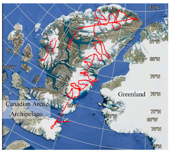
Figure 1.
The sites of data acquisition. The Arctic Archipelago is a group of islands along the Canadian Arctic Ocean; the glacial channels in the Arctic Archipelago are usually narrower than 3000 m.

Table 1.
MCoRDS system parameters.
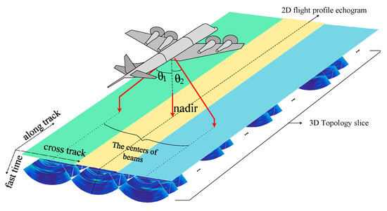
Figure 2.
Illustration of the imaging process of the MCoRDS. The topology slices are collected by three beams emitted by the MCoRDS. The flight direction of the aircraft is the along-track direction (range line), the cross-track direction (elevation angle bin) is perpendicular to the along-track direction and the fast-time axis (range bin) is perpendicular to both the along-rack direction and the cross-track direction.
The radar topology sequence [41] collected by the MCoRDS is shown in Figure 3 and Figure 4. Figure 3 shows a frame in a segment of 3D topology terrain sequence data. The horizontal axis represents the cross-track elevation angles discretized into direction-of-arrival bins (that is, the radar scanning width) and the vertical axis represents the fast time dimension, i.e., range bin. The most important structure in each radar topology slice is the ice-surface layer, which is the interface between air and ice, and the ice-bottom layer, which represents the boundary between ice bottom and bedrock. It can be found, from Figure 3, that the ice layer in the echo map is a fuzzy area, accounting for a small part of the total image area, and it is not easy to distinguish the specific location of ice layers from the echogram. A segment of the 3D topology sequence consists of a series of continuous ice sheet radar topology slices, which can reconstruct a complete target terrain, as shown in Figure 4. On the left, a segment of slices is presented and a 3D terrain reconstructed from these slices is shown on the right.
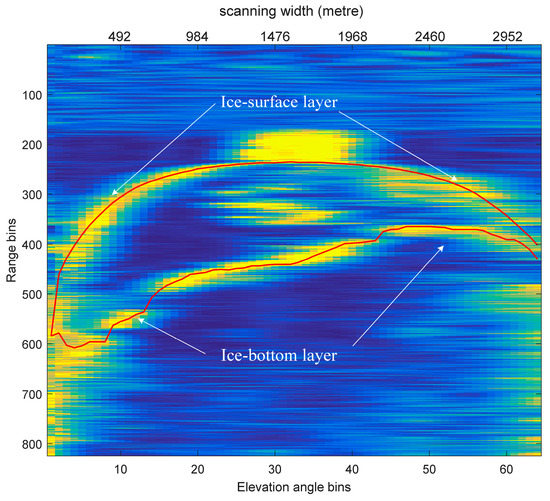
Figure 3.
Illustration of a topology slice with two kinds of labels, ice-surface layer and ice-bottom layer. White arrows indicate the ice-surface layer and ice-bottom layer. The red lines are the locations of ice-surface layer and ice-bottom layer (ground truth) marked by human expert.
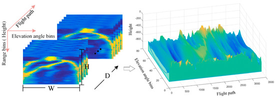
Figure 4.
Illustration of a segment of 3D radar topology sequences (left) and a 3D sub-glacial terrain (right) reconstructed from the sequence. H and W are the height and width of each topology slice, respectively, and D is the number of slices in a segment.
3.2. Network Framework
As shown in Figure 5, the MsANet is divided into three stages: low-level feature extraction, discriminatory high-level feature extraction and classification. Low-level feature extraction is used to learn the common features of the ice-surface and ice-bottom layers; high-level feature extraction is applied to learn features of the ice-surface and ice-bottom layers; in classification, the estimation of the ice layer locations according to learned features from the first two stages are output. To better learn the unique characteristics of the ice-surface and ice-bottom layers, a two-branch architecture [38] is used and an improved C3D network, C3D-M, ensures the spatial relativity of learned features. To further enhance the feature extraction capability and avoid the pre-mature fusion of relationships between radar sequences, adjustable multi-scale modules (Msks) are introduced in all blocks, except block 1, in the feature extraction stage. To refine the features of layers, improved 3D attention modules, which can collect global semantic correlations, are introduced in high-level feature extraction, in which two branches specialize in learning ice-surface and ice-bottom features, respectively. Moreover, the attention and multi-scale modules are fused to form an attention multi-scale module and further learn multi-scale layer features of topology sequences.
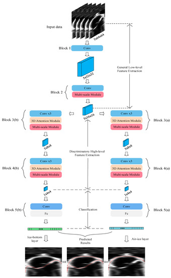
Figure 5.
The whole framework of the MsANet. The MsANet, which is divided into 5 blocks, consists of improved C3D-M inserted with proposed Msks and 3D attention modules. The blue cuboid is the feature maps with a size of A × B × C (depth × width × height); for example, the first one after block 1 is the feature maps with a size of 5 × 32 × 32.
The MsANet contains five types of blocks. After sequential slices are fed into the MsANet, the general low-level features of two layers are learned in shallow block 1 and the convolution unit, cascaded with an Msk in block 2, is used to further learn multi-scale information of low-level features. Discriminatory features of the ice-surface and ice-bottom layers are separately extracted by blocks 3 and 4, respectively, in the parallel branches. After the features pass through multiple convolution units in blocks 3 and 4, they are sent to the attention multi-scale module, in which features are first processed by the attention module to select key features, and the Msk is then used to learn the scale information of key features. Finally, in the classification part (block 5) of the two branches, estimations of the ice-surface and ice-bottom layers are performed according to the learned advanced features. Each branch outputs the estimated result of ice layers and the combination of these results is the final estimation of the ice layers.
3.3. Architecture of C3D-M
Since 3D convolution could simultaneously learn 3D features, a 3D convolution network [39] with compact feature extraction ability is selected as the backbone. A dual-branch structure [38] is adopted and improved to form the C3D-M network, which has two modifications. First, to retain more distinguishing features, mixed pooling (Mp) units are introduced into each feature extraction block, using the element summations of 3D maximum pooling and 3D average pooling. Second, the first full connection layer (Fc) in block 5 is replaced by a convolution unit (Conv), to ensure the spatial relativity of the collected features, and a full connection layer directly estimates the position of each ice layer.
As shown in Figure 6, the improved C3D-M structure consists of five blocks. The first two blocks learned common low-level features in ice sheet radar images. From the third block, C3D-M is divided into two branches to learn discriminatory features of air-surface and ice-bottom layers. Classification with block 5 was performed to output the estimation of ice layers. In the feature extraction stage, the convolution unit is 3 × 5 × 3 and the Mp unit is 1 × 2 × 2. The numbers of the convolution filters in blocks 1–5 are 16, 32, 64, 128 and 128, respectively.

Figure 6.
Improved C3D-M structure with 16, 32, 64 and 128 output channels per block. Numbers in brackets are the orders of convolution in blocks. Mp: mixed pooling.
3.4. Multi-Scale Module
The Msk uses multiple branches with different scale convolution to learn features in different deep directions (the deep direction is the same as the sequence direction). As shown in Figure 7, the Msk is composed of the K branch 3D convolution units with different depths to collect more scale information, a bottleneck unit for channel transformation and an Mp unit. The K branch could be adjusted according to the input to obtain different sequence information. The convolution filter sizes of K branches are 1 × 1 × 1, 3 × 3 × 3, …, × 3 × 3, where is an odd number and the maximum of is the number of input data frames.
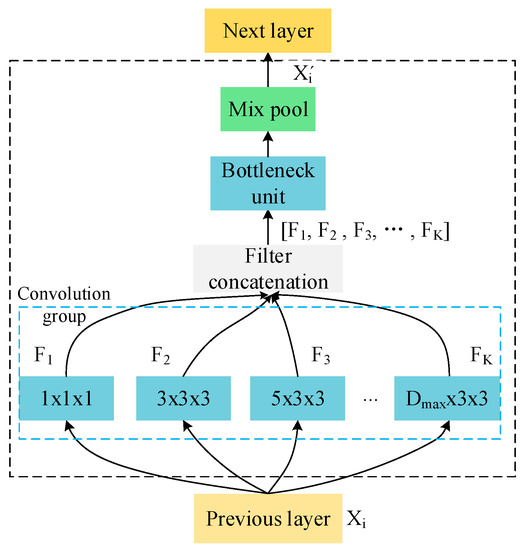
Figure 7.
Msk with K branches. The blue rectangle represents convolution and the green rectangle represents maximum pooling.
3.5. 3D Attention Module
To refine important features of ice layers, inspired by the position attention module (PAM) and channel attention module (CAM) of Fu et al. [34], a 3D attention module is proposed, which extends PAM and CAM to PAM3D and CAM3D, respectively, in 3D space, to learn 3D attention features. Unlike the attention module with C1, C2, C6, C7 and C8 bottleneck units [34], PAM3D and CAM3D are used with C1, C2, C6 and C7 bottleneck units; a C8 unit is not included because it easily confuses the useful features and reduces the distinctive features of the two layers. Equal numbers of channels in bottleneck units, whose filter size is the same as that of Fu et al. [34] and which is extended to 3D, were used in the improved 3D attention module to learn more features.
As shown in Figure 8, the proposed 3D attention module is divided into two parallel branches. The extracted features are sent to parallel bottleneck units (C1, C2) for feature transformation and features are fed to PAM3D and CAM3D in parallel to learn information from different aspects. PAM3D uses three 1 × 1 × 1 convolution units (C3, C4 and C5) to learn features, K, Q and V, and assigns a location weight E [34], in which data are extended to 3D. In CAM3D, 3D features are processed, such as reshaping, transposing and other operations [34], to generate channel weights . After flowing through PAM3D and CAM3D, a convolution unit (C6, C7) is used and element summation is performed to generate final attention features.
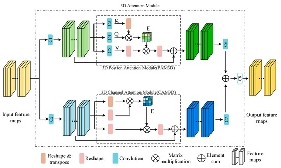
Figure 8.
Illustration of the 3D attention module structure. The 3D attention module structure is made up of two branches, the upper branch is the 3D position attention module and the lower one is the 3D channel attention module. are the feature maps with attention weights. In our attention module, the C8 unit, whose original placement position is indicated by the light-blue dashed box, used in [34] is deleted.
4. Experiment and Discussion
We describe the basic settings of the experiments in Section 4.1. Ablation experiments for each module are described in Section 4.2. The results of the MsANet are compared to those of other layer-finding methods in Section 4.3. The results of the MsANet are visualized in Section 4.4. In order to further verify the effectiveness of the MsANet, more experiments are shown in Section 4.5.
4.1. Datasets and Settings
Dataset and data preprocessing. A total of 8 segments of 2014 CAA data obtained by CReSIS [41], each containing 3332 topological slices, is used for training and testing. Each slice corresponds to a true label image. The total number of used slices or true label images is 8 × 3332 = 26,656. Each slice is resized from 824 × 64 to 64 × 64 by bicubic interpolation to reduce the number of parameters and the running time. Five consecutive frames are randomly selected from topological sequences as input. The input size is 1 × 5 × 64 × 64, i.e., one input channel and five slices of size 64 × 64.
Before the data are fed to the network, they are preprocessed with the same method of [38]. The data in each slice are normalized to [−1, 1] and subtract the data mean value computed from the training images. The ground truth of each frame, that is, the absolute coordinates labels of the ice layer position in every single column of each frame, is normalized as in Equation (1):
where represents the ground truth of the i-th column of the “s” frame in the “m” segment, and and H signifies the height of each image before resize.
Implementation. All experiments were performed on a GTX 2080Ti, with 60% of the 8 segments of data randomly chosen for training and the remainder for testing. The basic learning rate was 0.0001, attenuating by half every five epochs, with an L1 loss function and Adam optimizer to update parameters, with a batch size of 64.
Metric. The average mean absolute column-wise error (average mean error) is calculated as:
where is the ground-truth value of the i-th column of each frame (note, the number of segment and slice are omitted, which is the same as in Equation (1)), is the estimation result of the corresponding column using the MsANet, W is the column width of each input image, d is the number of input frames and n = 3 is the number of times of training from scratch.
4.2. Ablation Experiments
We verify the effect of the backbone C3D-M and describe the experiments on the performance of branches in the Msk. We discuss the effectiveness of different positions of the improved 3D attention module and verify the influence of the C8 unit in the improved 3D attention module.
4.2.1. Choice of the Backbone Network
Table 2 shows the effects of backbone networks, which use different structures in the classification stage. The effects of the C3D network using two full connection layers are shown in columns 1–3, using the results of the experiments with 512 channels [38] in column 1 as a baseline. Columns 4–6 show the performance of the improved C3D-M networks, which combine a convolution unit with different channels and a full connection layer in the classification stage. “Air” is the average mean error of the ice-surface layer extracted by networks, “bed” is the average mean error on the ice-bottom layer and “sum” is the sum of “air” and “bed”. Using the same evaluation as Xu et al. [38], we also used the comprehensive results for comparison. The improved C3D-M network, which uses a convolution unit and a full connection layer with 256 channels, is the best, with 1.71 fewer pixels than the baseline. Experiments show that combining a convolution unit and a full connection layer is more effective than two full connection layers with the same channels. From the experiments, the combination of a convolution unit and a full connection layer is seen to be important. The C3D-M network with 256 channels is selected as the backbone of the MsANet.

Table 2.
Experiments on different classification structures.
4.2.2. Multi-Scale Module
To evaluate the effect of the Msk, C3D-M is used as the backbone and combinations of different scale filters are tested, with results as shown in Table 3. The baseline is the result of the C3D-M backbone. To make comparisons under the same conditions, the same 5-frame input is used as a baseline, so the number of branches in the Msk is K = 3. Experiments show that, for radar topology slices, combinations of filters with different sequence ranges have different effects and more scale filters bring better results. A 3-branch Msk has the most obvious extraction effect, whose result is 0.47 pixel lower than the baseline.

Table 3.
Ablation study of filter sizes in branches in Msks. The symbol of ”√” in the form means which method is used.
To verify the performance of more branches in the Msk, the results of 3- and 4-branch Msks with seven frames of input are tested, with results as shown in Table 4. The first row is the baseline generated by the C3D-M network, followed by the effects of different numbers of branches in the Msk. It can be seen that the 4-branch multi-scale module performed best, whose result is 0.62 pixel less than the baseline and 0.06 pixel less than that of the 3-branch. Although the 4-branch Msk performs best, it requires more parameters than the 3-branch, with small improvement. Considering the extraction result and parameters, the Msk with K = 3 branches is adopted.

Table 4.
Results of different branches in Msks with 7-frame input data.
4.2.3. 3D Attention Module
Table 5 shows the effects of PAM3D and CAM3D in different positions of the backbone. The first line is the baseline generated by the backbone C3D-M network with a 3-branch Msk inserted. Considering that the attention module shows better performance on higher-level features, we first experimented with PAM3D and CAM3D in block 4 to verify their effect. The results of experiments in lines 2–4 show that using PAM3D or CAM3D alone in the network is effective and their combination performed better than networks using a single attention module. The position effect of the combination of PAM3D and CAM3D is shown in lines 4–6. These experiments indicate that combinations in various positions show different improvements and, when the combination of PAM3D and CAM3D is placed in blocks 3 and 4, they show mutual promotion, with results 0.83 pixel less than the baseline. In the improved 3D attention module, PAM3D and CAM3D are simultaneously used in blocks 3 and 4.

Table 5.
Performance of attention modules in different positions. The symbol of “√” in the form means which method is used.
Table 6 shows the results of experiments on the necessity of C8 units in the 3D attention module. The first row is the baseline generated by the C3D-M network with Msks and 3D attention modules without bottleneck units. Row 2 shows the results with bottleneck units, except C8, and row 3 shows the effects of experiments with bottleneck units, including the C8 unit. It can be found that the results with bottleneck units except C8 are best, with a reduction of 0.74 pixels compared to the baseline. Results in rows 1 and 3 show that bottleneck units could improve the effect of 3D attention modules, but the results in rows 2 and 3 show that the C8 bottleneck does not make sense. Based on our experiments, the C8 unit is not used.

Table 6.
Experiments with and without C8 unit in attention module. The symbol of ”√” in the form means which method is used.
4.3. Comparison and Discussion with Other Methods
To better evaluate the effect of MsANet, which consists of a C3D-M with inserted Msks and 3D attention modules, it is compared to other methods on the average mean absolute column-wise error, numbers of parameters and speed, as shown in Table 7. Lee et al. [20] and Xu et al. [21] used traditional methods, with a Markov random field to realize layer-finding through different reasoning methods. However, Lee et al. [20] used technology originally designed for layer inference of 2D images, which did not consider the relationship between topological slices, and Xu et al. [21] decided to extract the ice-bottom layer from the radar topological sequence and introduced additional evidence from other sources of data, e. g., the “ice mask.” Xu et al. [38] used C3D and RNN networks to extract ice-surface layer and ice-bottom layer from radar tomographic sequences. For a fair comparison, the ice mask information is removed from Xu et al. [21] and this is marked with an asterisk (“*”).

Table 7.
Results compared with other methods using 8 segments of data to train and test. The method marked with “*” is the method of Xu et al. [21] which removes the ice mask information.
As shown in Table 7, the MsANet has the lowest average mean error summed across the two layers, the fastest running time and the minimum number of parameters. The traditional methods [20,21] are inferior on the “bed” of average mean error under the same conditions, while DL methods ([38] and the MsANet) perform better in less time. The result of the MsANet is 2.14 pixels less than that of Xu et al. [38] on the sum of the two layers, the MsANet uses 12.48 M fewer parameters and the MsANet runs faster. Evaluated on the two ice layers alone, the MsANet has the best results of the ice-surface layer and is second on the ice-bottom layer. Although the result of bedrock identification by the MsANet is slightly inferior to that of Xu et al. [38], our method uses less computational time for a better comprehensive effect.
4.4. Visualization of Results
The results of the MsANet are visualized for direct observation. The three sets of extracted topological slices with the estimated position of the ice layers are shown in Figure 9. The red line represents the position of the estimated ice-surface layer and the green line is the position of the ice-bottom layer boundary. The first row shows the human-labeled ground truth of radar topology images, the second and third rows visualize the results extracted by Xu et al. [38] and the MsANet, respectively. The results of the MsANet are better than those of Xu et al. [38]; for example, the MsANet can learn the prior constraint relationships between ice layers, whose identified ice-bottom layer does not exceed the ice-surface layer, as shown in Figure 9b. In most part of 3D topology slices, the MsANet can effectively identify the smooth boundaries of the layers, while in weak echo parts of 3D topology slices, the layers extracted by the MsANet are not precise enough, as shown in the right of Figure 9c.
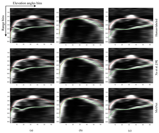
Figure 9.
Visualization of radar topology slices. (a–c): Three set of comparison of extracted ice-surface layer positions and ice-bottom layer positions obtained by human labeled, method of Xu et al. [38], and method of MsANet. For better viewing, images are converted to gray-scale. The red line indicates the ice-surface layer and the green one is the ice-bottom layer. The width direction represents the elevation angle bins and the height direction represents the range bins, which is the same as the fast-time axis.
The comparison of the ice layer details extracted by Xu et al. [38] and the MsANet is shown in Figure 10. The first column on the left is the extracted results of Xu et al. [38], while the fifth column is the extracted results of the MsANet and the middle three columns are respectively zoomed portions of the results extracted by Xu et al. [38], human-labeled and the MsANet for finer resolution analyses and comparisons. It can be seen that the layers extracted by the MsANet are closer to the ground truth than Xu et al. [38] in most part of the 3D ice sheet radar topology slices, such as the zoomed portion of (a) and (b) and the left part of the zoomed portion of (c). However, in parts of the 3D ice sheet radar topology slices, especially in strongly noisy parts, such as the right part of the zoomed portion in (c), both methods of Xu et al. [38] and the MsANet cannot correctly identify the ice position. Parts of the reconstructed ice-surface layer and ice-bottom layer structures are shown in Figure 11a,b.
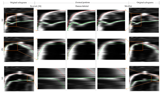
Figure 10.
Visualization of comparisons of zoomed portions of the extraction results of Xu et al. [38] and the MsANet. (a–c): Three set of comparison of extracted zoomed ice-surface layer positions and ice-bottom layer positions obtained by human labeled, method of Xu et al. [38], and method of MsANet.
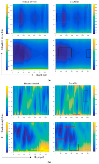
Figure 11.
Reconstructions of terrain from results extracted by the MsANet without any interpolation method. Unit: meter. (a) Ice-surface layer. (b) Ice-bottom layer. The x-axis in each image means the flight path and the y-axis is the scanning width of the MCoRDS, while the color indicates the elevation of layers, which is the depth from the radar. For better observation, red boxes are used to mark the part where the MsANet extracted results are close to the ground truth and black boxes are applied to highlight the part where the MsANet extracted results are not similar to the ground truth.
Figure 12a,b display, respectively, the elevation difference between the layers reconstructed by ground truth and reconstructed layers by the MsANet on the ice-surface layer and on the ice-bottom layer, that is, the elevation of reconstructed layers by ground truth minus the elevation of reconstructed layers by the MsANet, respectively, on the ice-surface layer and the ice-bottom layer. The reconstructed layers by the MsANet have similar appearances to the ground truth and the elevation difference of reconstructed ice layers between human-labeled and the MsANet are close to zero in most places. Only in the edge parts of the elevation difference images between the ground truth and reconstructed layers by the MsANet, there are some differences. As shown in Figure 12b, there are relatively higher elevation differences in the yellow area between the two dashed lines of the second elevation difference image. When the corresponding topological slices are analyzed, it is found that they are so blurred on their right part that it is difficult to clearly determine the ice-bedrock layer positions.
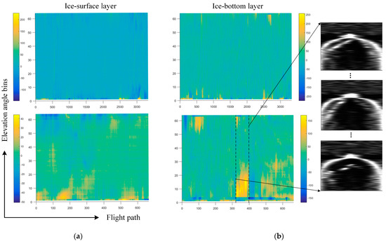
Figure 12.
Elevation differences of reconstructed layers using the results extracted by the MsANet. Unit: meter. (a) Elevation differences of the ice-surface layer. (b) Elevation differences of the ice-bottom layer. The topology slices between the two dashed lines in (b) are displayed on the right.
4.5. Extended Experiments
To further verify the effectiveness of the MsANet, more data, 97 segments of Canadian Arctic Archipelago (CAA) basal terrain topological slice data (other five segments with different numbers of slices are not considered), are used for training and testing with different divisions of training sets and test sets, respectively: (1) 60% of 97 segments for training, the remaining 40% for testing; (2) about 75% of 97 segments for training, the remaining 25% for testing. The parameters and settings of the MsANet are the same as those in Section 4.1.
It can be found, from Table 8, that with the increase in training data, the extraction results of the two networks are constantly improved and the performance of the MsANet is better than that of Xu et al. [38]. The numbers in brackets indicate the improvement on the evaluation of “sum” of the networks (Xu et al. [26] and the MsANet) using different proportions of training sets. After making the same change to the training data, the improvement of the MsANet results (10.5%) is higher than that of Xu et al. [38] (7.5%) on the evaluation of “sum”. In general, our MsANet is also better than the method of Xu et al. [38] in the expanded dataset.

Table 8.
Experimental results with different divisions of 97 segments data.
5. Conclusions
We propose the MsANet framework to extract and reconstruct ice layers from radar topological sequences at less cost. The MsANet combines multi-scale and attention modules, using an improved 3D convolution network as the backbone, to better learn the scale information of key features extracted from the ice-surface and ice-bottom layers to estimate them. Experiments showed that, compared to state-of-the-art DL methods, the MsANet can better learn the constraints between ice layers and it has better performance in the extraction of clear boundaries, its estimation of ice layers on the edges of images is closer to the ground truth and it can identify parts of ambiguous ice layer structures. However, the extraction ability of bedrock is poor, perhaps due to the lack of a learning relationship of wide-range topological sequences. Our future work will further consider the integration of wide-range topological sequence relationships to optimize the extraction of the location of the ice-bedrock layer and take into account the convolution long short-term memory network to gain better performance.
Author Contributions
Conceptualization, Y.C., S.L., X.C. and D.L.; methodology, Y.C. and D.L.; validation, D.L.; formal analysis, D.L., J.X. and J.Y.; writing—original draft preparation, Y.C. and D.L.; writing—review and editing, Y.C., S.L., X.C., D.L., J.X. and J.Y. All authors have read and agreed to the published version of the manuscript.
Funding
This research was funded by the National Key Research and Development Program of China (no.2017YFC1703302) and the National Natural Science Foundation of China (no. 41776186).
Institutional Review Board Statement
Not applicable.
Informed Consent Statement
Not applicable.
Data Availability Statement
Not applicable.
Conflicts of Interest
The authors declare no conflict of interest.
References
- Mackay, A. Climate Change 2007: Impacts, Adaptation and Vulnerability. Contribution of Working Group II to the Fourth Assessment Report of the Intergovernmental Panel on Climate Change (ICPP AR4). J. Environ. Qual. 2008, 37, 2407. [Google Scholar] [CrossRef]
- Randolph Glacier Inventory 6.0. Available online: http://www.glims.org/RGI/randolph60.html (accessed on 21 April 2021).
- Gilbert, A.; Flowers, G.E. Sensitivity of Barnes Ice Cap, Baffin Island, Canada, to climate state and internal dynamics. J. Geophys. Res. Earth Surf. 2016, 121, 1516–1539. [Google Scholar] [CrossRef]
- England, J.; Smith, I.R. The last glaciation of east-central ellesmere island, nunavut: Ice dynamics, deglacial chronology, and sea level change. Can. J. Earth Sci. 2000, 37, 1355–1371. [Google Scholar] [CrossRef][Green Version]
- DeFoor, W.; Person, M. Ice sheet–derived submarine groundwater discharge on Greenland's continental shelf. Water Resour. Res. 2011, 47, W07549. [Google Scholar] [CrossRef]
- Nick, F.; Vieli, A. Large-scale changes in Greenland outlet glacier dynamics triggered at the terminus. Nat. Geosci. 2009, 2, 110–114. [Google Scholar] [CrossRef]
- Fretwell, P.; Pritchard, H.D. Bedmap2: Improved Ice Bed, Surface and Thickness Datasets for Antarctica. Cryosphere 2013, 7, 375–393. [Google Scholar] [CrossRef]
- Morlighem, M.; Williams, C.N. BedMachine v3: Complete bed topography and ocean bathymetry mapping of Greenland from multibeam echo sounding combined with mass conservation. Geophys. Res. Lett. 2017, 44, 11051–11061. [Google Scholar] [CrossRef] [PubMed]
- Beltrami, H.; Taylor, A.E. Records of climatic changes in the Canadian Arctic: Towards calibrating oxygen isotope data with geo-thermal data, Global Planet. Change 1995, 11, 127–138. [Google Scholar]
- Grootes, P.M.; Stuiver, M. Comparison of oxygen isotope records from the GISP2 and GRIP Greenland ice cores. Nature 1993, 366, 552–554. [Google Scholar] [CrossRef]
- Souney, J.M.; Twickler, M.S. Core handling, transportation and processing for the south pole ice core (spicecore) project. Ann. Glaciol. 2020, 62, 118–130. [Google Scholar] [CrossRef]
- Bogorodsky, V.V.; Bentley, C.R. Radioglaciology, 1st ed.; D. Reidel Publishing Company: Dordrecht, The Netherlands, 1985; pp. 8–10. [Google Scholar]
- Nixdorf, U.; Steinhage, D.; Meyer, U. The newly developed airborne radio-echo sounding system of the awi as a glaciological tool. Ann. Glaciol. 1999, 29, 231–238. [Google Scholar] [CrossRef]
- Conway, H.; Hall, B.L. Past and Future Grounding-Line Retreat of the West Antarctic Ice Sheet. Science 1999, 286, 280–283. [Google Scholar] [CrossRef] [PubMed]
- Bamber, J.L.; Layberry, R.L. A new ice thickness and bed data set for the Greenland ice sheet. J. Geophys. Res. 2001, 106, 33773–33780. [Google Scholar] [CrossRef]
- Anschütz, H.; Sinisalo, A. Variation of accumulation rates over the last eight centuries on the East Antarctic Plateau derived from volcanic signals in ice cores. J. Geophys. Res. 2011, 116, D20103. [Google Scholar] [CrossRef]
- Freeman, G.J.; Bovik, A.C.; Holt, J.W. Automated detection of near surface Martian ice layers in orbital radar data. In Proceedings of the 2010 IEEE Southwest Symposium on Image Analysis & Interpretation (SSIAI), Austin, TX, USA, 23–25 May 2010; IEEE: New York, NY, USA. [Google Scholar]
- Mitchell, J.E.; Crandall, D.J.; Fox, G.C. A semi-automatic approach for estimating near surface internal layers from snow radar imagery. In Proceedings of the 2013 IEEE International Geoscience and Remote Sensing Symposium (IGARSS), Melbourne, VIC, Australia, 21–26 July 2013; IEEE: New York, NY, USA. [Google Scholar]
- Gifford, C.M.; Finyom, G. Automated Polar Ice Thickness Estimation from Radar Imagery. IEEE Trans. Image Process. 2010, 19, 2456–2469. [Google Scholar] [CrossRef] [PubMed]
- Crandall, D.J.; Fox, G.C.; Paden, J.D. Layer-finding in radar echograms using probabilistic graphical models. In Proceedings of the 21st International Conference on Pattern Recognition (ICPR), Tsukuba, Japan, 11–15 November 2012; IEEE: New York, NY, USA, 2012. [Google Scholar]
- Lee., S.; Mitchell, J.; Crandall, D.J. Estimating bedrock and surface layer boundaries and confidence intervals in ice sheet radar imagery using MCMC. In Proceedings of the 2014 IEEE International Conference on Image Processing (ICIP), Paris, France, 27–30 October 2014; IEEE: New York, NY, USA. [Google Scholar]
- Xu, M.; Crandall, D.J.; Fox, G.C. Automatic estimation of ice bottom surfaces from radar imagery. In Proceedings of the 2017 IEEE International Conference on Image Processing (ICIP), Beijing, China, 17–20 September 2017; IEEE: New York, NY, USA. [Google Scholar]
- Berger, V.; Xu, M. Automated Ice-Bottom Tracking of 2D and 3D Ice Radar Imagery Using Viterbi and TRW-S. IEEE JSTARS 2019, 12, 3272–3285. [Google Scholar] [CrossRef]
- Al-Ibadi, M.; Sprick, J.; Athinarapu, S. DEM extraction of the basal topography of the Canadian archipelago ICE caps via 2D automated layer-tracker. In Proceedings of the 2017 IEEE International Geoscience and Remote Sensing Symposium (IGARSS), Fort Worth, TX, USA, 23–28 July 2017; IEEE: New York, NY, USA. [Google Scholar]
- Zhao, H.; Shi, J.; Qi, X. Pyramid Scene Parsing Network. In Proceedings of the 2017 IEEE Conference on Computer Vision and Pattern Recognition (CVPR), Honolulu, HI, USA, 21–26 July 2017; IEEE: New York, NY, USA. [Google Scholar]
- He, M.; Li, B.; Chen, H. Multi-scale 3D deep convolutional neural network for hyperspectral image classification. In Proceedings of the 2017 IEEE International Conference on Image Processing (ICIP), Beijing, China, 17–20 September 2017; IEEE: New York, NY, USA. [Google Scholar]
- Chen, L.C.; Zhu, Y.; Papandreou, G. Encoder-decoder with atrous separable convolution for semantic image segmentation. In Proceedings of the 15th European Conference on Computer Vision (ECCV), Munich, Germany, 8–14 September 2018; Springer: Cham, Switzerland. [Google Scholar]
- Song, L.; Zhang, S.; Yu, G.; Sun, H. TACNet: Transition-Aware Context Network for Spatio-Temporal Action Detection. In Proceedings of the 2019 IEEE/CVF Conference on Computer Vision and Pattern Recognition (CVPR), Long Beach, CA, USA, 15–20 June 2019; IEEE: New York, NY, USA. [Google Scholar]
- Zhang, W.; He, X. A Multi-Scale Spatial-Temporal Attention Model for Person Re-Identification in Videos. IEEE Trans. Image Process. 2020, 29, 3365–3373. [Google Scholar] [CrossRef] [PubMed]
- Xu, K.; Ba, J.L.; Ryan, K. Show, attend and tell: Neural image caption generation with visual attention. In Proceedings of the 32nd International Conference on International Conference on Machine Learning (ICML), Lille, France, 6–11 July 2015. [Google Scholar]
- Yang, X.; Zhang, B.; Dong, Y. Spatiotemporal Attention on Sliced Parts for Video-based Person Re-identification. In Proceedings of the 2018 IEEE Visual Communications and Image Processing (VCIP), Taichung, Taiwan, 9–12 December 2018. [Google Scholar]
- Woo, S.; Park, J.; Lee, J. Cbam: Convolutional block attention module. In Proceedings of the 15th European Conference on Computer Vision (ECCV), Munich, Germany, 8–14 September 2018; Springer: Cham, Switzerland. [Google Scholar]
- Wang, X.; Girshick, R.; Gupta, A. Non-local Neural Networks. In Proceedings of the 2018 IEEE/CVF Conference on Computer Vision and Pattern Recognition (CVPR), Salt Lake City, UT, USA, 18–22 June 2018. [Google Scholar]
- Fu, J.; Liu, J.; Tian, H. Dual Attention Network for Scene Segmentation. In Proceedings of the IEEE/CVF Conference on Computer Vision and Pattern Recognition (CVPR), Long Beach, CA, USA, 15–20 June 2019; pp. 3141–3149. [Google Scholar]
- Cho, K.; Van Merriënboer, B.; Gulcehre, C.; Bahdanau, D.; Bougares, F.; Schwenk, H.; Bengio, Y. Learning Phrase Representations using RNN Encoder—Decoder for Statistical Machine Translation. arXiv 2014, arXiv:1406.1078. Available online: https://arxiv.org/pdf/1406.1078v3.pdf (accessed on 12 March 2020).
- Kamangir, H.; Rahnemoonfar, M.; Dobbs, D. Deep Hybrid Wavelet Network for Ice Boundary Detection in Radra Imagery. In Proceedings of the 2018 IEEE International Geoscience and Remote Sensing Symposium (IGARSS), Valencia, Spain, 22–27 July 2018; IEEE: New York, NY, USA. [Google Scholar]
- Cai, Y.H.; Hu, S.B. End-to-end classification network for ice sheet subsurface targets in radar imagery. Appl. Sci. 2020, 10, 2501. [Google Scholar] [CrossRef]
- Xu, M.; Fan, C.; Paden, J.D. Multi-Task Spatiotemporal Neural Networks for Structured Surface Reconstruction. In Proceedings of the 2018 IEEE Winter Conference on Applications of Computer Vision (WACV), Lake Tahoe, NV, USA, 12–15 March 2018; IEEE: New York, NY, USA, 2018. [Google Scholar]
- Tran, D.; Bourdev, L.; Fergus, R. Learning Spatiotemporal Features with 3D Convolutional Networks. In Proceedings of the 2015 IEEE International Conference on Computer Vision (ICCV), Santiago, Spain, 7–13 December 2015; IEEE: New York, NY, USA, 2015; pp. 4489–4497. [Google Scholar]
- Paden, J.; Akins, T. Ice-Sheet Bed 3-D Tomography. J. Glaciol. 2010, 56, 3–11. [Google Scholar] [CrossRef]
- CReSIS. Available online: http://data.cresis.ku.edu/ (accessed on 12 December 2020).
Publisher’s Note: MDPI stays neutral with regard to jurisdictional claims in published maps and institutional affiliations. |
© 2021 by the authors. Licensee MDPI, Basel, Switzerland. This article is an open access article distributed under the terms and conditions of the Creative Commons Attribution (CC BY) license (https://creativecommons.org/licenses/by/4.0/).