Abstract
Automatic remote sensing (RS) image to map translation is a crucial technology for intelligent tile map generation. Although existing methods based on a generative network (GAN) generated unannotated maps at a single level, they have limited capacity in handling multi-resolution map generation at different levels. To address the problem, we proposed a novel conditional scale-consistent generation network (CscGAN) to simultaneously generate multi-level tile maps from multi-scale RS images, using only a single and unified model. Specifically, the CscGAN first uses the level labels and map annotations as prior conditions to guide hierarchical feature learning with different scales. Then, a multi-scale discriminator and two multi-scale generators are introduced to describe both high-resolution and low-resolution representations, aiming to improve the similarity of generated maps and thus produce high-quality multi-level tile maps. Meanwhile, a level classifier is designed for further exploring the characteristics of tile maps at different levels. Moreover, the CscGAN is optimized by jointly multi-scale adversarial loss, level classification loss, and scale-consistent loss in an end-to-end manner. Extensive experiments on multiple datasets and study areas demonstrate that the CscGAN outperforms the state-of-the-art methods in multi-level map translation, with great robustness and efficiency.
1. Introduction
Electronic maps are of great importance for urban computing and location-based services like navigation, autonomous vehicles and so on. However, electronic maps are mainly traditionally obtained through field surveys or manual image interpretation, which is time-consuming and labor-intensive. Hence, automatically, electronic map production is of great value in addressing these limitations and is widely considered [1,2,3,4,5,6,7,8,9,10,11]. Recently, domain mapping or image-to-image translation based methods have been intensively focused and applied to automatic electronic map production, which automatically and efficiently targets translating remote sensing (RS) images to tile maps [2,3,4]. Although promising results have been achieved in one-level map translation [2,3,4,8], simultaneously creating multi-level tile maps remains several challenges, such as scale variation, text annotation loss and ground target change in different levels (see Figure 1). To address these challenges, we propose the CscGAN, a novel deep generation network that can simultaneously translate multi-scale RS images to the corresponding tile maps of different levels, with significant robustness and efficiency.
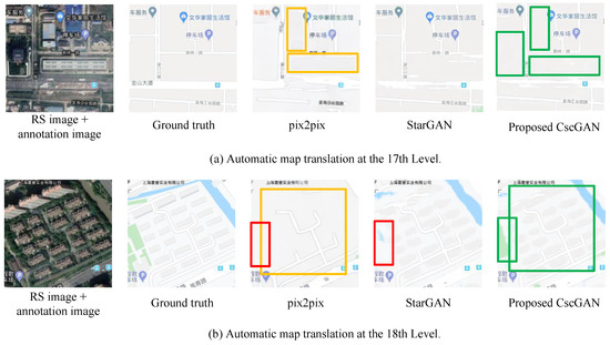
Figure 1.
Generated results at multiple levels using different models. (a) Automatic map translation at the 17th Level. From left to right: RS image + annotation image, Ground truth, by pix2pix, by StarGAN and by the proposed CscGAN. (b) Automatic map translation at the 18th Level. From left to right: RS image + annotation image, Ground truth by pix2pix, by StarGAN and by the proposed CscGAN. Note: in generated mappings, red rectangles represent loss contents; yellow rectangles represent confused contents; green rectangles represent the correct contents generated by the proposed method.
Electronic map production generally can be divided into the following two categories: traditional computer-aided cartography-based methods and deep learning-based methods. Computer-aided cartography usually includes four stages, namely map designation, data input, symbolized editing and graphic output. However, in the process of computer-aided map production, a lot of work still depends on manual expert participation and professional tools such as ArcGIS and MapGIS [1], the production cycle and cost of which are relatively high. Therefore, it is very difficult to quickly generate large-range or even city-level electronic maps.
Recently, deep learning-based methods have been intensively developed for automatically multi-level map translation, due to its strong capacity of feature representation and generation ability [2,3,4,12]. It significantly simplifies the overall process and labour cost of map production and provides the possibility to quickly generate large-range electronic maps. Existing deep learning-based methods can be divided into the following two broad categories: one-to-one mappings [2,3,4,13,14] and many-to-many mappings [5,6,15]. The one-to-one mapping-based methods, such as pix2pix [2], CycleGAN [3] and GcGAN [4], use the source domain image as an input condition and then use one generator to output the target domain image. Meanwhile, one discriminator output the real or fake probability of the target domain image. The many-to-many mapping-based methods, such as StarGAN [5] and its improved versions [6], can simultaneously generate multi-domain images based on different target labels. Although these solutions have achieved satisfactory results in image-to-image translation, it’s still difficult to directly use them for multi-level tile map generation, mainly due to the following two limitations.
- One-to-one mapping-based methods usually use two ways to implement map generation with multiple levels, that is, separated training at each level and uniform training with multiple levels. For the former way, tile maps at each level are trained separately, which makes the time and space complexity of the model very high. Meanwhile, due to the low utilization of the training set during the separated training, a larger amount of training samples are needed. For the latter way, the unified training of RS images with different levels can easily cause multi-level information confusion and detailed information loss at a finer level. As shown in Figure 1, the uniformly trained pix2pix did not discriminate RS images from which levels, resulting in generating the confusing contents at the 17th level (maybe from the 18th level), meanwhile, the loss of important contents such as the green land at the finer level (see the red rectangles in Figure 1).
- Many-to-many mapping-based methods usually use one generator and auxiliary information to complete multi-level map generation, leading to the errors of detailed content generated at higher levels. For example, as shown in Figure 1, although the StarGAN generated the green land at the 18th level map, the generated land contained a lot of false information and also lost a lot of details (see the red rectangle in the Figure 1b).
To address the above-mentioned limitations in multi-level map translation, we proposed a novel conditional scale-consistent GAN (CscGAN) that simultaneously generates multi-level tile maps from multi-scale RS images, using only a single and unified model with great robustness and efficiency. The CscGAN consists of a multi-scale generator, two multi-scale discriminators, and a map-level classifier, where the annotation images with level labels are used as the prior conditions to guide the network for hierarchical feature generation.
The main contributions of this paper are as follows:
- A single and unified multi-level map generation model, called CscGAN, is proposed to learn the mappings among multiple levels, training effectively and efficiently from multi-scale RS images and annotation images with different levels and resolutions. As far as we know, this is the first model to simultaneously generate different tile maps in multiple levels.
- Two multi-scale discriminators and a multi-scale generator are designed for jointly learning both high-resolution and low-resolution representations, aiming to produce high-quality tile maps with rich details at different levels.
- A map-level classifier is introduced to guide the network for discriminating the learned representations from which level, improving the stability and efficiency of adversarial training in multi-level map generation.
- We construct and label a new RS-image-to-map dataset for multi-level map generation and analysis referred to as the “self-annotated RS-image-to-map dataset”. Extensive experiments on two datasets and cross study areas show that the CscGAN outperforms the state-of-the-art methods for the quality of different levels of map translation.
The remainder of this paper is organized as follows: Section 2 describes related work. Section 3 introduces the details of the used dataset in this study. Section 4 presents the proposed CscGAN for tile map generation with multiple levels in detail. Section 5 discusses the experimental results on publicly available and self-annotated datasets and study areas. Finally, this paper is concluded in Section 6.
2. Related Work
In this section, methods that are related to Image-to-Image translation and tile map translation are discussed.
2.1. Image-to-Image Translation
Image-to-Image translation has been a recent development and research hotspot in the field of generative adversarial network (GAN) [12]. GAN based Image-to-Image translation generally consists of a generator and discriminator that play games during training, to achieve Nash equilibrium and finally to generate the fake data. It’s known that it is a challenge to optimize the generator and discriminator in GAN during training [16,17,18]. To address this problem, a lot of training algorithms have been developed for novel generative tasks over the past few years. DCGAN [19] used a convolutional neural network as the generative network and proposed a series of suggestions so that GAN is more stable in training. WGAN [16] adopted the Wasserstein distance to the objective function of the GAN, which can effectively solve gradient vanishes or gradient explosion during training. WGAN-GP [20] directly restricted the gradient of the discriminator based on WGAN. LSGAN [21] also modified the objective function and changed the classification task to a regression task in the discriminator, which can effectively solve gradient vanishing. Additionally, to produce high-resolutional images, existing methods, such as [13,22,23,24,25], first produced lower resolution images and then reproduced them into higher resolution images.
2.2. Automatic Map Translation from RS Images
Automatic map translation from RS images has recently attracted more and more attention from academia and industry [26]. Pix2pix [2] is first used in map translation. It used RS images as the generator’s input to generate the corresponding Google map and then used the generated Google map to train the discriminator. The recently proposed CycleGAN architecture has been evaluated on RS image to map translation [3], which does not need pairing data by adding a cycle consistency loss. Similar to CycleGAN, GcGAN [4] proposed a geometric consistency constraint GAN to generate maps from RS images. GANs have been also used to create spoof satellite images and spoof images of the ground truth conditioned on the satellite image of the location [27]. Conditional GANs have also been used to generate ground-level views of locations from overhead satellite images Deng, Zhu, and Newsam [28]. Semantic segmentation has also been used to predict the probabilities from spectral features of the RS images [7,8,9]. It is very similar to map translation.
In general, the existing methods mostly generated high-quality unannotated maps at a single level, and the generation of more detailed text annotations at multiple levels is still an open research problem.
3. Materials
3.1. Maps Dataset
The maps dataset is widely used in RS image-to-map translation task [2,4,29,30]. The data were collected from Google Maps at a single level. In the experiments, 1096 RS images and 1096 electronic tile maps are used together for training, and 1098 RS images and 1098 electronic tile maps are used for testing. Table 1 shows the maps dataset for the training, the testing in our experiment. Note that the dataset has no level attribute. Some examples from the map dataset are shown in Figure 2.

Table 1.
Detailed information for the training and testing.
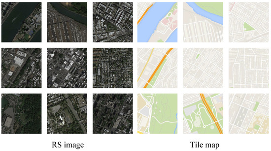
Figure 2.
Examples from the maps dataset.
3.2. Self-Annotated RS-Image-to-Map Dataset and Study Areas
This dataset was collected, annotated and built independently by the authors. The pairs of RS images, annotation images and maps with multiple levels scraped from Google Maps. The RS image, annotation image and the corresponding map for this dataset were collected from some regions in Shanghai and Hubei, China, covering 14, 15, 16, 17 and 18 levels, respectively. In this dataset, there are 1476 pairs of tile images (namely maps and RS images) at each level, where the size of each tile is 256 × 256 pixels. Figure 3 shows examples with different levels from the dataset, and Table 2 lists the detailed information of the dataset.
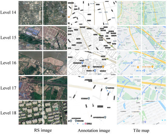
Figure 3.
Examples from the self-annotated RS-image-to-map dataset at different levels, namely from the 14 to 18 levels.
Table 2.
Detailed information on the self-annotated RS-image-to-map dataset and study areas.
In this study, since the number and resolution in lower levels is insufficient for training, for example, there are only 506 tile maps at level 8 in China, we chose the levels from 14 to 18. Additionally, the data split for training (1230 pairs), validation (123 pairs), test sets (123 pairs), and the total number of samples (1476 pairs) at each level in the experiments. Table 1 gives detailed training and testing schemes for the self-annotated RS-image-to-map dataset.
To evaluate the performance of the different areas, we selected two study areas in Shanghai (including, Songjiang District, Pudong New District, Minhang District, Qingpu District) and Hubei (including Wuhan city, Yingcheng city, Xiaogan city, Huanggang city), respectively. These two areas are relatively developed in China, with intricate roads and rich annotated information, which are very suitable for map translation evaluation. Table 2 shows the detailed information of the study areas, including the latitude, longitude range, scale and spatial resolution at each level.
4. Methods
In this section, a brief overview of the proposed end-to-end CscGAN for multi-scale RS images to multi-level map translation is first presented. Then, the learning process of each component of the approach is described.
4.1. The Overview of the Method
In this paper, we propose a new multi-level map translation network (termed CscGAN) based on multi-scale RS images and their annotation images, which incorporates a multi-scale generator, two multi-scale discriminators, and a map-level classifier into a GAN framework, as shown in Figure 4. CscGAN allows simultaneous training of multi-level RS data with different scales within a single network, where the annotation images with level labels are used as prior conditions to guide the network to perform hierarchical feature learning. Specifically, given an RS image x and its annotation image with the level label c as the conditional input, the multi-scale generator G is optimized to produce tile map distributions with two different resolutions via using two residual blocks of different scales as, (see the proposed CscGAN training pipeline in Figure 4). Meanwhile, two multi-scale discriminator are optimized to respectively distinguish the generated maps and real tile maps for learning the hierarchical features at different levels, where i represents the scale and j represents the features. Furthermore, the map-level classifier is introduced to guide the whole network for learning the map representations most relevant to the corresponding level according to the conditional input. Overall, high-quality tile maps with rich details at different levels can be simultaneously translated by the CscGAN with the following objective functions,
where and respectively are the loss of multi-scale discriminator and generator. x is a real RS image from the true data distribution , and y is a tile map from distribution . p is the number of generated branches, and we set in all of our experiments. and are hyper-parameters that control the relative importance of level classification loss and distance loss during training, respectively. We set and in all of our experiments, similar to [2]. In order to stabilize the training process, we use the least-squares loss [21] instead of the traditional objective function in GAN.
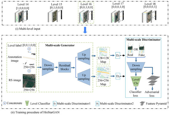
Figure 4.
The architecture of the proposed CscGAN.
Each component in the CscGAN is subsequently introduced in detail.
4.2. Multi-Scale Generator
Due to resolution variation in both RS images and tile maps at different levels, the traditional generator in GANs has difficulty generating both high and low resolution maps directly due to overfitting and unstable training [24]. Therefore, a multi-scale generator G with two parallel scale branches is designed for generating multi-resolution maps of different levels, aiming to model both high-resolution and low-resolution image feature distributions at the same time and overwhelm overfitting during training. The detailed architecture of the proposed multi-scale generator is presented in Figure 5. It consists of a backbone adopted in CycleGAN [30] and two scale generated branches (see and in Figure 5). In the small-scale branch , the generator first generates low-resolution tile maps according to basic color and structures via two stride-2 convolutions and 7 residual blocks, and thus some detailed text annotations might be omitted; then, in the large-scale branch , the generator focuses on previously ignored text information to generate higher resolution maps.
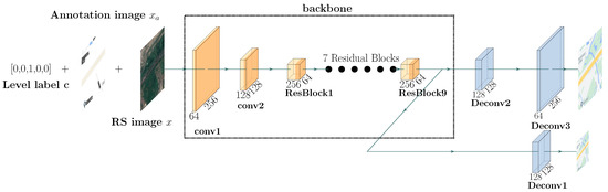
Figure 5.
The architecture of the multi-scale generator.
Specifically, the small-scale branch outputs a lower resolution map with the size of 128 × 128, and the large-scale branch outputs the higher resolution map with the size of 256 × 256. To effectively learn discriminative representations with different resolution at each branch, a multi-scale adversarial loss function is proposed and calculated as follows:
where , and respectively represent the RS image, annotation image and its map with the ith resolution. is the multi-scale discriminator described in the following section. Additionally, the multi-scale generator is to not only fool the discriminator but also approach the ground truth via the following scale-consistent distance loss at each scale:
It forces the generated map to be near the prior annotation map at each scale.
4.3. Multi-Scale Discriminator
Since the multi-scale generator produces maps of two different resolutions (see the above Section 3.1), two multi-scale discriminators, i.e., and in the Figure 4, are adopted to respectively connect to the above two generator branches ( and ), to explicitly enforce the CscGAN to learn better alignment between the RS image and the conditioning text annotation images at multiple levels. The framework of each multi-scale discriminator is shown in Figure 6. For each multi-scale discriminator , we first use PatchGAN [2,3] as the backbone, which classifies each patch of an image as real or fake. However, some detailed information may be lost in this process. To alleviate information loss, each multi-scale discriminator is designed as a tree-like structure, which contains three sub-discriminators to hierarchically learn features of different levels. Since multi-resolution images were generated by two generated branches, two discriminators were used for different scales.
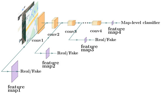
Figure 6.
The architecture of each multi-scale discriminator.
During training, each discriminator takes real RS images and their corresponding text annotation images as positive sample pairs. The total multi-scale adversarial loss is used to optimize the two multi-scale discriminators and is defined as follows:
where m is the total number of sub-discriminators in each multi-scale discriminator and is set as 3 in this study. j represents the jth sub-discriminator. Additionally, the total multi-scale adversarial loss is the average for all generator branches.
Finally, the proposed multi-scale discriminator learns multi-resolution probability distributions over both input source x, , and discriminate the tile map y, that is, . Besides, is the proposed map-level classifier that is used to classify input data into the relevant level, which will be described below.
4.4. Map-Level Classifier
In this section, a map-level classifier is introduced to guide the network for discriminating the learned representations from which level. To make use of the prior conditions, the map-level classifier M is plunged into the top of the multi-scale discriminator D, as shown in Figure 7, improving the stability and efficiency of adversarial training for map generation at different levels.
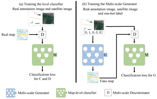
Figure 7.
The training procedure of the map-level classifier. G represents the multi-scale generator, M represents the map-level classifier, and D represents the multi-scale discriminator. (a) The real image goes through D and then into M to calculate the classification loss and optimize the classifier and the multi-scale discriminator . (b) G generates a map based on the input RS image, annotation image and level label. Then, M calculates the classification loss of the generator and optimizes the multi-scale generator.
Figure 7 illustrates the training process of the map-level classifier and the multi-scale generator. Given the level label c, a one-hot vector is first used to encode c as for categorical attributes. Then, a level classification loss of real images is used to optimize the classifier and the multi-scale discriminator , while a level classification loss of fake images is used to optimize multi-scale generator G. In detail, the map-level classification loss of real images is given by
where the factor represents a probability distribution over map level labels computed by the map-level classifier . and represent RS images and tile maps at the ith resolution branch, respectively. Through minimizing this objective , can classify a real RS image to its corresponding level c. Additionally, the map-level classification loss of the fake images is defined as
where is the ith generator branch in the multi-scale generator. It can classify the generated fake images to the relevant level c by minimizing this objective function.
The level classifier contained three stride-1 convolutions and four stride-2 convolutions. The output size of the level classifier was 1 × 1 × N, where N represents the number of levels in the experiments.
5. Experiments and Analysis
In this section, we thoroughly evaluate the proposed approach on two challenging pair datasets, that is, the public maps dataset and a self-annotated RS-image-to-map dataset, and two different study areas including Shanghai and Wuhan in China.
5.1. Evaluation Metrics
To quantitatively and thoroughly evaluate the proposed model, we also perform quantitative evaluation using the following metrics: Peak Signal to Noise Ratio (PSNR) [31], Structural Similarity (SSIM) [31,32], Pixel Accuracy [4], and the metrics in a classification task (Accuracy, Precision, Recall, F1 score).
5.1.1. Peak Signal to Noise Ratio (PSNR)
PSNR directly measures the difference in pixel values. Suppose x and y represent the pixel values from the generated image and the original image, respectively. The size of each image is pixels. The mean squared error (MSE) is first calculated as:
where i and j define the pixel index positions in an image. Then, the PSNR can be expressed as
where is the maximum possible pixel value of the image. For example, each pixel is represented by an 8 bit in binary; then, equals .
5.1.2. Structural Similarity (SSIM)
SSIM estimates the holistic similarity between two images. SSIM is designed by modelling any image distortion as a combination of the following three factors: loss of structure, luminance distortion, and contrast distortion [31,32]. The SSIM is calculated as:
where
Equation (11) is the luminance comparison function. It is used to measure the closeness of the average luminance of two images (x and y). This factor is equal to 1 only if . Equation (12) is the contrast comparison function. It is used to measure the closeness of the contrast between the two images (i.e., x and y). The standard deviation measures the contrast and . This term is equal to 1 only if . Equation (13) is the structure comparison function. It is used to measure the correlation coefficient of image x and image y [31]. Note that is the covariance between the two images x and y. The positive value of the SSIM index is in . Zero means there is no correlation between images; one means . To avoid a null denominator, bring into three positive constants , , and .
5.1.3. Pixel Accuracy
The third evaluation metric is used in GcGAN [4], which is used to assess the accuracy of aerial photo to map translation. Formally, given a pixel i with the ground-truth RGB value (,,) and the predicted RGB value (,,), the pixel accuracy (acc) is computed as
Since maps only contain a limited number of different RGB values, it is reasonable to compute pixel accuracy using this strategy ( = 5 in this paper).
5.1.4. Accuracy, Precision, Recall, F1 Score, ROC Curves
As with other classification tasks, we use Accuracy, Precision, Recall, F1 Score to evaluate the level classifier’s performance as follows:
We also use the receiver operating characteristic (ROC) curve as the level classifier’s performance indicators.
5.2. Implementation Details
5.2.1. Training Details
CscGAN was implemented using the Pytorch deep learning framework [33]. We adopted mini-batch SGD and applied the Adam solver with a batch size of 1, a learning rate of 0.0002, and momentum parameters = 0.5, = 0.999.
5.2.2. Experimental Machine Configuration
The network models were trained on a PC with an Intel (R) Core™ i7-6700 CPU at 4.00 GHz with 32 GB memory and an NVIDIA GeForce RTX 2080. All the models are tested on an NVIDIA GeForce GTX 960M.
5.3. Evaluation of Maps Dataset
The proposed CscGAN was compared with existing state-of-the-art methods, including pix2pix [2] and CycleGAN [30] on the maps dataset, as shown in Table 3. The pix2pix uses an RS image x to realize the translation from the RS image x to the tile map y. CycleGAN also achieves translation from the RS image x to tile map y, but the data requirements are not as strict as pix2pix. The PSNR [31], SSIM [31,32], and pixel accuracy [4] mentioned in Section 5.1 were used to evaluate these methods. Table 3 lists the experimental results, and Figure 8 shows the visualization results generated by the different methods on the maps dataset. Compared to the state-of-the-art methods, the proposed CscGAN achieved outperformance in all evaluation metrics.
Table 3.
Comparison of the state-of-the-art methods on the maps dataset. The best results are highlighted in bold.
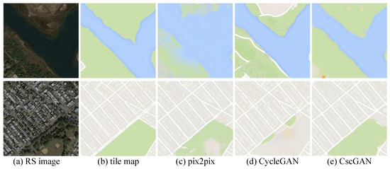
Figure 8.
Visualization generation results via different methods on maps dataset.
Since the maps dataset has only one level, the CscGAN here did not include the map-level classifier. The results generated by the CscGAN are more similar to the ground truth than those generated by the other methods. For PSNR, SSIM and pixel accuracy, our method increases by 0.611, 0.039, and 5.234%, respectively, compared to the second highest model(pix2pix). As shown in Figure 8c,d, both the pix2pix and CycleGAN cannot generate large areas such as rivers and green space well. The rivers and green spaces generated by CscGAN significantly outperformed the other methods. It is proved that the multi-scale generator enables the network to obtain more detailed information.
5.4. Evaluation of the Self-Annotated RS-Image-to-Map Dataset
Table 4 reports the comparison results of pix2pix [2], CycleGAN [30], StarGAN [5], and the proposed CscGAN on the self-annotated RS-image-to-map dataset. Since this dataset includes five levels, the one-to-one mapping-based methods, like pix2pix and CycleGAN, need to be trained as five independent models. As shown in Table 4, the proposed CscGAN exhibited significantly improved performance for multi-levels map generation in several evaluation metrics. Compared to existing methods, our method has the largest growth in PSNR, SSIM and pixel accuracy over 5%, 0.18% and 13% respectively. We conjecture that multi-scale generator and multi-scale discriminator can model more detailed information so that the CscGAN can generate better results at multiple levels. Additionally, Table 5 lists the total parameter sizes and inference time of the different models. Compared to other methods, the proposed CscGAN has smaller parameter sizes (only 81.5 MB), which makes training time much less than other methods. The tiny increase of reference time shows that the proposed CscGAN can achieve the best performance with tiny additional computational cost, which means that the proposed method can achieve an excellent balance between accuracy and efficiency.
Table 4.
The results of different methods evaluated on the RS-image-to-map dataset. Acc represents pixel accuracy, which is mentioned in Section 5.1.3. Avg represents the average result of the five levels. Note that the best results are highlighted in bold.
Table 5.
The total parameter sizes and inference time of the different methods. Note that the best results are highlighted in bold.
In addition, due to space limitations, in Figure A1, we show the generated results of different methods at each level. Compared to the CycleGAN and pix2pix, the CscGAN produced more detailed and precise contents in tile maps. Furthermore, compared to the results of StarGAN, the CscGAN also achieved competitive visualization results at multiple levels, especially detailed contents such as text annotations and subtle loads in the high-level maps.
5.5. Ablation Experiment and Study
The impact of each component in CscGAN on the final performance is verified in this section. Table 6 presents the ablation results of the gradual addition of the level classifier, multi-scale discriminator and multi-scale generator training on the baseline pix2pix [2] framework. The results of ablation experiments were quantified by PSNR [31], SSIM [32], and pixel accuracy [4]. As seen from Table 6, after adding the map-level classifier, the PSNR, SSIM and pixel accuracy are remarkably higher (respectively increases by 0.521%, 0.018%, 1.994%) than the baseline. After adding the multi-scale discriminator, the PSNR achieved the increment (about 0.114). The possible reason is that the improvement of the discriminator’s ability indirectly leads to the enhancement of the generator’s ability. Finally, adding the multi-scale generator, the PSNR, SSIM and pixel accuracy are remarkably higher (increases by 0.01%, 0.004%, 1.183%). In addition to improving the quality of the generated results, the multi-scale approach can effectively enhance the stability of GAN training, especially in the generation of high-resolution images.
Table 6.
Ablation study of the proposed CscGAN. Impact of integrating our different components (Level Cls, Mult D, and Mult G) into the baseline on the RS-image-to-map dataset for ablation experiments. +Map-level Cls: Add a level classifier to pix2pix. +Mult D: Add a multi-scale discriminator based on the previous model. +Mult G: Add a multi-scale generator based on the previous model. Note: The best results are presented in bold.
Furthermore, Figure 9d shows the generated visualization results, with using multi-scale and not using multi-scale generator. As shown in Figure 9d, without using the multi-scale generator, the training process was very unstable, resulting in the very terrible results. On the contrary, with using the multi-scale generator, the problem of training instability is alleviated and thus the correct maps can be generated (see Figure 9e).
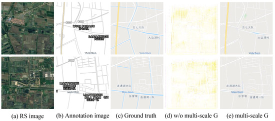
Figure 9.
The comparison of generation results with the use of the multi-scale generator and without the use of the multi-scale generator.
To further study the effectiveness of the level classifier, Figure 10 and Figure 11 respectively provide the confusion matrixes and ROC curve of real-fake map classification in the level classifier on the self-annotation RS-image-to-map dataset. From Figure 10a, we can be observed that the map-level classifier reached an accuracy of 94.8%, precision of 94.97%, recall of 94.8%, and F1 score of 0.95 for real map classification. Additionally, we used the multi-scale generator to generate a fake map as the input into the level classifier. The classified results by the level classifier are shown in Figure 10b. Most of the fake maps can be successfully classified to the corresponding level by the level classifier (the accuracy is 89.27%, the precision is 90.14%, recall is 89.27%, and F1 score is 0.89). Moreover, Figure 12a,b respectively presents the generated maps at the 17th, 18th level, whether using the level classifier. Obviously, the level classifier makes the generated map details richer and more accurate.
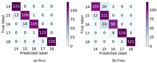
Figure 10.
The classification results by the level classifier. (a) The confusion matrix of classification on the real data; (b) the confusion matrix of classification on the fake data.
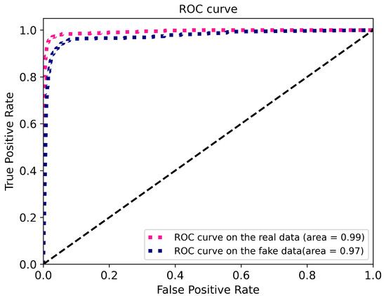
Figure 11.
ROC curve by the level classifier.
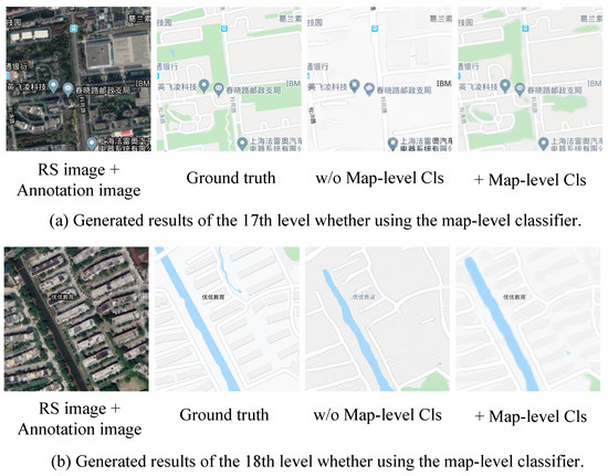
Figure 12.
The comparison of generation results with the use of the map-level classifier and without the use of the map level classifier.
5.6. Generalization Analysis of Cross Study Areas
To verify the generalization ability of the proposed CscGAN in different areas, we used RS images in the Shanghai area for training and the Hubei area for testing. Table 2 lists the training and testing information of the used study areas. The comparison experiments were conducted by pix2pix [2], CycleGAN [30], StarGAN [5], and CscGAN on the cross study areas. Table 7 reports the evaluation results of the PSNR [31], SSIM [32] and pixel accuracy [4] for the three models.
Table 7.
The generalization results via different methods, we use the study areas in Shanghai for training while other areas in Wuhan for testing. Note that the best results are highlighted in bold.
Compared to the other state-of-the-art methods, the results of the proposed CscGAN demonstrate that it can be better reused for multi-level map generation in other study areas. For SSIM, the highest results were achieved by the proposed CscGAN at each level. For PSNR and Acc, compared to the StarGAN at the 17th and 18th levels, although the results of the proposed method slightly declined, the average results of the three metrics were significantly improved (increases by 0.039%, 0.003%, 0.456%). Additionally, to clarify the visualization quality of the generation maps, generation results at each level can be shown in Figure A2. The CscGAN has a good effect on detailed information generation at finer levels, e.g., rivers, text annotations, and green areas.
5.7. Result Analysis and Discussion of Study Areas with Different Levels
To clearly discuss the quality of generated maps from large RS images at different levels, Figure 13, Figure 14, Figure 15, Figure 16 and Figure 17 exhibit the qualitative results from the level 14 to level 18 in different districts in Shanghai. Four study districts (Songjiang District, Pudong New District, Minhang District and Qingpu District) were selected to investigate the effectiveness of the proposed algorithm.
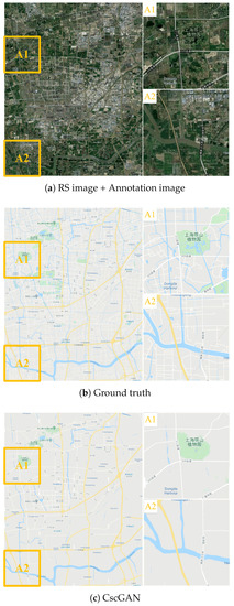
Figure 13.
The generation results with level 14 via the proposed CscGAN in Songjiang District of Shanghai. For clarity, the zoomed local areas (A1 and A2) are on the right of the figure.
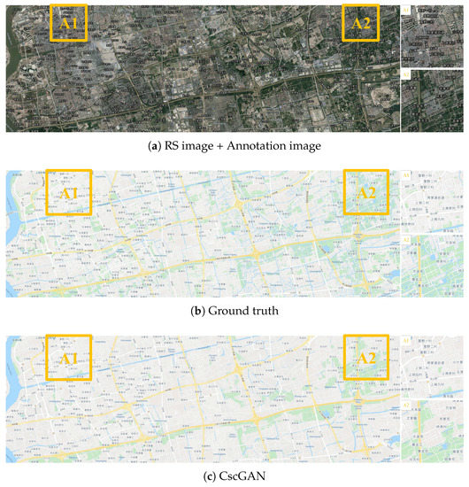
Figure 14.
The generation results with level 15 via the proposed CscGAN in the Pudong New Area of Shanghai. For clarity, the zoomed local areas (A1 and A2) are on the right of the figure.
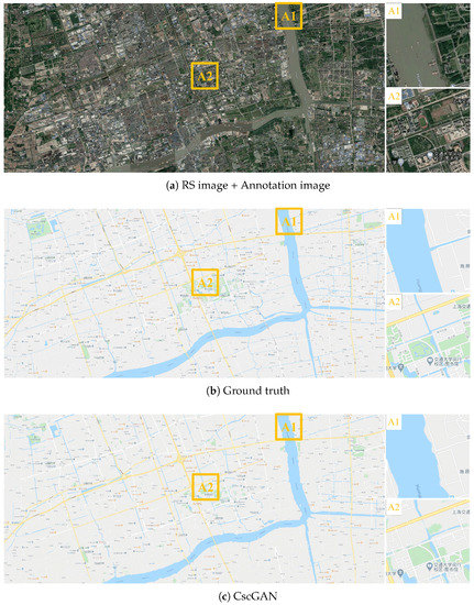
Figure 15.
The generation results with level 16 via the proposed CscGAN in Minhang District of Shanghai. For clarity, the zoomed local areas (A1 and A2) are on the right of the figure.
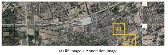
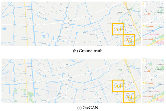
Figure 16.
The generation results with level 17 via the proposed CscGAN in Qingpu District of Shanghai. For clarity, the zoomed local areas (A1 and A2) are on the right of the figure.
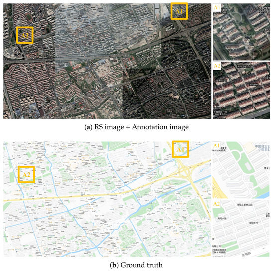
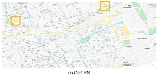
Figure 17.
The generation results with level 18 via the proposed CscGAN in Minhang District of Shanghai. For clarity, the zoomed local areas (A1 and A2) are on the right of the figure.
Figure 13 presents the large RS image, annotation image, ground truth, and generated map in Songjiang District of Shanghai at the 14th level, where the results generated by the proposed CscGAN are very similar to the RS image and the ground truth. The generated results in Figure 13c show that both the coarse information including green land, rivers, and some rough roads and the detailed information including map annotations and words, are similar to the ground truth. For clarity, the zoomed local areas (A1 and A2) are on the right of the figure. Note that, because there is slight mismatch between RS images and real maps (see Figure 13a,b), the low resolution images at the 14th level are difficult to distinguish the fake or real features by the discriminator.
Figure 14 exhibits the maps generated by the proposed CscGAN in the Pudong New Area of Shanghai at the 15th level. Through observation, it can be found that the finer roads generated at the 15th level are finer than at the 14th level.
Additionally, Figure 15, Figure 16 and Figure 17 respectively depict the generation results with levels 16 to 18 in Minhang District and Qingpu District, in Shanghai. With the finer level, detailed annotations and content in RS images become finer, so the generation maps are clearer and more accurate than previous levels. Moreover, the generated lettering annotations were verisimilitude at each level.
6. Conclusions
This paper proposed an end-to-end trainable map generation network, termed CscGAN, to perform high-quality map generation with multiple levels from multi-scale RS images using only a single and unified model. In CscGAN, we designed two multi-scale discriminators and a multi-scale generator to jointly learn both high-resolution and low-resolution representations with rich details at different levels, and a map-level classifier to further guide the network for learning the map representations most relevant to the corresponding level. Furthermore, to carry out experiments at different map levels, we constructed a new dataset with multiple level RS images, annotation images and corresponding tile maps. Experiments on two map datasets (namely the maps dataset and the self-annotated RS-image-to-map dataset) and two different study areas (i.e., Songjiang District, Pudong New District, Minhang District, and Qingpu District in Shanghai and Wuhan, Yingcheng, Xiaogan, Huanggang in Hubei) demonstrate that the CscGAN can simultaneously train multiple levels of data using a single model and achieve a much-improved performance and greater robustness than other methods. However, in finer levels, dense building contours are still easily blurred. In future work, a powerful edge-constrained network will be explored in our CscGAN framework, for providing a more reliable synthetic map.
Author Contributions
Conceived the foundation, Y.L.; designed the methods, Y.L. and W.W.; preformed the experiments, W.W.; interpretation of results, Y.L. and W.W.; writing-original draft preparation, Y.L. and W.W.; writing-review and editing, Y.L., F.F. and L.Z.; data curation, C.S. and Y.Z.; supervision, Z.C.; funding acquisition, Y.L. All authors have read and agreed to the published version of the manuscript.
Funding
This research was funded by National Natural Science Foundation of China grant (41871305, 62076227), a National key R & D program of China (No.2017YFC0602204), a Wuhan Applied Fundamental Frontier Project Grant (2020010601012166), the Fundamental Research Funds for the Central Universities, China University of Geosciences (Wuhan) (No.CUGQY1945), the Opening Fund of Key Laboratory of Geological Survey and Evaluation of Ministry of Education, China Aerospace Science and Industry Joint Foundation, and the Fundamental Research Funds for the Central Universities (No.GLAB2019ZR02).
Institutional Review Board Statement
Not applicable.
Informed Consent Statement
Not applicable.
Data Availability Statement
Publicly available datasets were analyzed in this study. This data can be found here: http://efrosgans.eecs.berkeley.edu/pix2pix/datasets/maps.tar.gz, accessed on 14 May 2021.
Acknowledgments
This work was partially supported by National Natural Science Foundation of China grant (41871305, 62076227), a National key R & D program of China (No.2017YFC0602204), a Wuhan Applied Fundamental Frontier Project Grant (2020010601012166), the Fundamental Research Funds for the Central Universities, China University of Geosciences (Wuhan) (No.CUGQY1945), the Opening Fund of Key Laboratory of Geological Survey and Evaluation of Ministry of Education, China Aerospace Science and Industry Joint Foundation, and the Fundamental Research Funds for the Central Universities (No.GLAB2019ZR02).
Conflicts of Interest
The authors declare no conflict of interest.
Appendix A

Figure A1.
Example results translated by different methods.
Figure A1.
Example results translated by different methods.


Figure A2.
Example results in the Wuhan area.
Figure A2.
Example results in the Wuhan area.

References
- Jing, Y. Research on Large Scale Vector Electronic Map Data Production Based on ArcGIS. Geomat. Spat. Inf. Technol. 2015, 38, 135–136. [Google Scholar]
- Isola, P.; Zhu, J.Y.; Zhou, T.; Efros, A.A. Image-to-Image Translation with Conditional Adversarial Networks. In Proceedings of the IEEE Conference on Computer Vision and Pattern Recognition, Honolulu, HI, USA, 21–26 July 2017; pp. 1125–1134. [Google Scholar]
- Zhu, J.Y.; Park, T.; Isola, P.; Efros, A.A. Unpaired Image-to-Image Translation Using Cycle-Consistent Adversarial Networks. In Proceedings of the IEEE International Conference on Computer Vision, Venice, Italy, 22–29 October 2017; pp. 2223–2232. [Google Scholar]
- Fu, H.; Gong, M.; Wang, C.; Batmanghelich, K.; Zhang, K.; Tao, D. Geometry-Consistent Generative Adversarial Networks for One-Sided Unsupervised Domain Mapping. In Proceedings of the IEEE Conference on Computer Vision and Pattern Recognition, Long Beach, CA, USA, 16–20 June 2019; pp. 2427–2436. [Google Scholar]
- Choi, Y.; Choi, M.; Kim, M.; Ha, J.W.; Kim, S.; Choo, J. StarGAN: Unified Generative Adversarial Networks for Multi-Domain Image-to-Image Translation. In Proceedings of the 2018 IEEE/CVF Conference on Computer Vision and Pattern Recognition, Salt Lake City, UT, USA, 18–23 June 2018; pp. 8789–8797. [Google Scholar] [CrossRef]
- Choi, Y.; Uh, Y.; Yoo, J.; Ha, J.W. Stargan v2: Diverse Image Synthesis for Multiple Domains. In Proceedings of the IEEE/CVF Conference on Computer Vision and Pattern Recognition, Seattle, WA, USA, 13–19 June 2020; pp. 8188–8197. [Google Scholar]
- Marmanis, D.; Wegner, J.D.; Galliani, S.; Schindler, K.; Datcu, M.; Stilla, U. Semantic segmentation of aerial images with an ensemble of CNSS. ISPRS Ann. Photogramm. Remote Sens. Spat. Inf. Sci. 2016 2016, 3, 473–480. [Google Scholar] [CrossRef]
- Wu, H.; Zhang, H.; Zhang, X.; Sun, W.; Zheng, B.; Jiang, Y. DeepDualMapper: A gated fusion network for automatic map extraction using aerial images and trajectories. Proc. AAAI Conf. Artif. Intell. 2020, 34, 1037–1045. [Google Scholar] [CrossRef]
- Kaiser, P.; Wegner, J.D.; Lucchi, A.; Jaggi, M.; Hofmann, T.; Schindler, K. Learning aerial image segmentation from online maps. IEEE Trans. Geosci. Remote Sens. 2017, 55, 6054–6068. [Google Scholar] [CrossRef]
- Hinz, S.; Baumgartner, A. Automatic extraction of urban road networks from multi-view aerial imagery. ISPRS J. Photogramm. Remote Sens. 2003, 58, 83–98. [Google Scholar] [CrossRef]
- Hu, J.; Razdan, A.; Femiani, J.C.; Cui, M.; Wonka, P. Road Network Extraction and Intersection Detection From Aerial Images by Tracking Road Footprints. IEEE Trans. Geosci. Remote Sens. 2007, 45, 4144–4157. [Google Scholar] [CrossRef]
- Goodfellow, I.; Pouget-Abadie, J.; Mirza, M.; Xu, B.; Warde-Farley, D.; Ozair, S.; Courville, A.; Bengio, Y. Generative Adversarial Nets. In Advances in Neural Information Processing Systems; MIT Press: Cambridge, MA, USA, 2014; pp. 2672–2680. [Google Scholar]
- Wang, T.C.; Liu, M.Y.; Zhu, J.Y.; Tao, A.; Kautz, J.; Catanzaro, B. High-Resolution Image Synthesis and Semantic Manipulation with Conditional Gans. In Proceedings of the IEEE Conference on Computer Vision and Pattern Recognition, Salt Lake City, UT, USA, 18–22 June 2018; pp. 8798–8807. [Google Scholar]
- Yi, Z.; Zhang, H.; Tan, P.; Gong, M. Dualgan: Unsupervised Dual Learning for Image-to-Image Translation. In Proceedings of the IEEE International Conference on Computer Vision, Venice, Italy, 22–29 October 2017; pp. 2849–2857. [Google Scholar]
- Lin, Y.J.; Wu, P.W.; Chang, C.H.; Chang, E.; Liao, S.W. RelGAN: Multi-Domain Image-to-Image Translation via Relative Attributes. In Proceedings of the 2019 IEEE/CVF International Conference on Computer Vision (ICCV), Seoul, Korea, 27 October–2 November 2019; pp. 5913–5921. [Google Scholar] [CrossRef]
- Arjovsky, M.; Chintala, S.; Bottou, L. Wasserstein gan. arXiv 2017, arXiv:1701.07875. [Google Scholar]
- Arjovsky, M.; Bottou, L. Towards Principled Methods for Training Generative Adversarial Networks. Stat 2017, 1050, 17. [Google Scholar]
- Salimans, T.; Goodfellow, I.J.; Zaremba, W.; Cheung, V.; Radford, A.; Chen, X. Improved Techniques for Training GANs. arXiv 2016, arXiv:1606.03498. [Google Scholar]
- Radford, A.; Metz, L.; Chintala, S. Unsupervised Representation Learning with Deep Convolutional Generative Adversarial Networks. arXiv 2016, arXiv:1511.06434. [Google Scholar]
- Gulrajani, I.; Ahmed, F.; Arjovsky, M.; Dumoulin, V.; Courville, A.C. Improved Training of Wasserstein Gans. arXiv 2017, arXiv:1704.00028. [Google Scholar]
- Mao, X.; Li, Q.; Xie, H.; Lau, R.Y.; Wang, Z.; Paul Smolley, S. Least Squares Generative Adversarial Networks. In Proceedings of the IEEE International Conference on Computer Vision, Venice, Italy, 22–29 October 2017; pp. 2794–2802. [Google Scholar]
- Zhang, H.; Xu, T.; Li, H.; Zhang, S.; Wang, X.; Huang, X.; Metaxas, D.N. StackGAN: Text to Photo-Realistic Image Synthesis with Stacked Generative Adversarial Networks. In Proceedings of the IEEE International Conference on Computer Vision (ICCV), Venice, Italy, 22–29 October 2017. [Google Scholar]
- Zhang, H.; Xu, T.; Li, H.; Zhang, S.; Wang, X.; Huang, X.; Metaxas, D.N. Stackgan++: Realistic Image Synthesis with Stacked Generative Adversarial Networks. IEEE Trans. Pattern Anal. Mach. Intell. 2018, 41, 1947–1962. [Google Scholar] [CrossRef] [PubMed]
- Karras, T.; Aila, T.; Laine, S.; Lehtinen, J. Progressive Growing of GANs for Improved Quality, Stability, and Variation. arXiv 2017, arXiv:1710.10196. [Google Scholar]
- Karnewar, A.; Wang, O. Msg-Gan: Multi-Scale Gradients for Generative Adversarial Networks. In Proceedings of the IEEE/CVF Conference on Computer Vision and Pattern Recognition, Seattle, WA, USA, 13–19 June 2020; pp. 7799–7808. [Google Scholar]
- Li, J.; Chen, Z.; Zhao, X.; Shao, L. MapGAN: An Intelligent Generation Model for Network Tile Maps. Sensors 2020, 20, 3119. [Google Scholar] [CrossRef] [PubMed]
- Xu, C.; Zhao, B. Satellite Image Spoofing: Creating Remote Sensing Dataset with Generative Adversarial Networks (Short Paper). In Proceedings of the 10th International Conference on Geographic Information Science (GIScience 2018), Melbourne, Australia, 28–31 August 2018. [Google Scholar]
- Deng, X.; Zhu, Y.; Newsam, S. What is it like down there? Generating dense ground-level views and image features from overhead imagery using conditional generative adversarial networks. In Proceedings of the 26th ACM SIGSPATIAL International Conference on Advances in Geographic Information Systems, Seattle, WA, USA, 6–9 November 2018; pp. 43–52. [Google Scholar]
- Mao, Q.; Lee, H.Y.; Tseng, H.Y.; Ma, S.; Yang, M.H. Mode Seeking Generative Adversarial Networks for Diverse Image Synthesis. In Proceedings of the 2019 IEEE/CVF Conference on Computer Vision and Pattern Recognition (CVPR), Long Beach, CA, USA, 15–21 June 2019; pp. 1429–1437. [Google Scholar] [CrossRef]
- Chu, C.; Zhmoginov, A.; Sandler, M. CycleGAN, a Master of Steganography. arXiv 2017, arXiv:1712.02950. [Google Scholar]
- Hore, A.; Ziou, D. Image Quality Metrics: PSNR vs. SSIM. In Proceedings of the 2010 20th International Conference on Pattern Recognition, Istanbul, Turkey, 23–26 August 2010; pp. 2366–2369. [Google Scholar] [CrossRef]
- Wang, Z.; Bovik, A.C.; Sheikh, H.R.; Simoncelli, E.P. Image Quality Assessment: From Error Visibility to Structural Similarity. IEEE Trans. Image Process. 2004, 13, 600–612. [Google Scholar] [CrossRef] [PubMed]
- Paszke, A.; Gross, S.; Massa, F.; Lerer, A.; Bradbury, J.; Chanan, G.; Killeen, T.; Lin, Z.; Gimelshein, N.; Antiga, L.; et al. PyTorch: An Imperative Style, High-Performance Deep Learning Library. arXiv 2019, arXiv:1912.01703. [Google Scholar]


Publisher’s Note: MDPI stays neutral with regard to jurisdictional claims in published maps and institutional affiliations. |
© 2021 by the authors. Licensee MDPI, Basel, Switzerland. This article is an open access article distributed under the terms and conditions of the Creative Commons Attribution (CC BY) license (https://creativecommons.org/licenses/by/4.0/).