
Long-Term Variation in the Tropospheric Nitrogen Dioxide Vertical Column Density over Korea and Japan from the MAX-DOAS Network, 2007–2017

 , ,
, , 
Abstract
1. Introduction
2. Materials and Methods
2.1. Measurement Sites
2.2. MAX-DOAS Instruments
2.3. Retrieval Algorithms
2.4. Ozone Monitoring Instrument (OMI)
2.5. Potential Source Regions
3. Results and Discussion
3.1. Monthly Variation in the NO2 TropVCD from MAX-DOAS and OMI
3.2. Long-Term Trend in the NO2 TropVCD from OMI and MAX-DOAS
3.3. Diurnal Variation in the NO2 VCD below 1 km Altitude
3.4. Potential Source Region for the NO2 TropVCD at Yokosuka and Gwangju
4. Conclusions
Supplementary Materials
Author Contributions
Funding
Data Availability Statement
Acknowledgments
Conflicts of Interest
References
- Bond, D.W.; Zhang, R.; Tie, X.; Brasseur, G.P.; Huffines, G.R.; Orville, R.E.; Boccippio, D.J. NOxproduction by lightning over the continental United States. J. Geophys. Res. Space Phys. 2001, 106, 27701–27710. [Google Scholar] [CrossRef]
- Zhang, R.; Tie, X.; Bond, D.W. Impacts of anthropogenic and natural NOx sources over the U.S. on tropospheric chemistry. Proc. Natl. Acad. Sci. USA 2003, 100, 1505–1509. [Google Scholar] [CrossRef]
- Crutzen, P.J. The influence of nitrogen oxides on the atmospheric ozone content. Q. J. R. Meteorol. Soc. 1970, 96, 320–325. [Google Scholar] [CrossRef]
- Leighton, P. Photochemistry of Air Pollution; Elsevier: Amsterdam, The Netherlands, 2012. [Google Scholar]
- Finlayson-Pitts, B.J.; Pitts, J.N., Jr. Atmospheric Chemistry. Fundamentals and Experimental Techniques. Available online: https://www.osti.gov/biblio/6379212-atmospheric-chemistry-fundamentals-experimental-techniques (accessed on 13 May 2021).
- Zhao, B.; Wang, S.X.; Liu, H.; Xu, J.Y.; Fu, K.; Klimont, Z.; Hao, J.M.; He, K.B.; Cofala, J.; Amann, M.C. NOx emissions in China: Historical trends and future perspectives. Atmos. Chem. Phys. 2013, 13, 9869–9897. [Google Scholar] [CrossRef]
- Zhang, Q.; Streets, D.G.; He, K.; Wang, Y.; Richter, A.; Burrows, J.P.; Uno, I.; Jang, C.J.; Chen, D.; Yao, Z.; et al. NOxemission trends for China, 1995–2004: The view from the ground and the view from space. J. Geophys. Res. Space Phys. 2007, 112. [Google Scholar] [CrossRef]
- Liu, F.; Zhang, Q.; van der Ronald, J.A.; Zheng, B.; Tong, D.; Yan, L.; Zheng, Y.; He, K. Recent reduction in NO x emissions over China: Synthesis of satellite observations and emission inventories. Environ. Res. Lett. 2016, 11, 114002. [Google Scholar] [CrossRef]
- Georgoulias, A.K.; van der Ronald, J.A.; Stammes, P.; Boersma, K.F.; Eskes, H.J. Trends and trend reversal detection in 2 decades of tropospheric NO2 satellite observations. Atmos. Chem. Phys. 2019, 19, 6269–6294. [Google Scholar] [CrossRef]
- Jamali, S.; Klingmyr, D.; Tagesson, T. Global-Scale Patterns and Trends in Tropospheric NO2 Concentrations, 2005–2018. Remote Sens. 2020, 12, 3526. [Google Scholar] [CrossRef]
- Zheng, B.; Tong, D.; Li, M.; Liu, F.; Hong, C.; Geng, G.; Li, H.; Li, X.; Peng, L.; Qi, J.; et al. Trends in China’s anthropogenic emissions since 2010 as the consequence of clean air actions. Atmos. Chem. Phys. 2018, 18, 14095–14111. [Google Scholar] [CrossRef]
- Kurokawa, J.; Ohara, T. Long-term historical trends in air pollutant emissions in Asia: Regional Emission inventory in ASia (REAS) version 3. Atmos. Chem. Phys. 2020, 20, 12761–12793. [Google Scholar] [CrossRef]
- Heckel, A.; Richter, A.; Tarsu, T.; Wittrock, F.; Hak, C.; Pundt, I.; Junkermann, W.; Burrows, J.P. MAX-DOAS measurements of formaldehyde in the Po-Valley. Atmos. Chem. Phys. 2005, 5, 909–918. [Google Scholar] [CrossRef]
- Hönninger, G.; Von Friedeburg, C.; Platt, U. Multi axis differential optical absorption spectroscopy (MAX-DOAS). Atmos. Chem. Phys. 2004, 4, 231–254. [Google Scholar] [CrossRef]
- Pinardi, G.; Van Roozendael, M.; Abuhassan, N.; Adams, C.; Cede, A.; Clémer, K.; Fayt, C.; Frieß, U.; Gil, M.; Herman, J.; et al. MAX-DOAS formaldehyde slant column measurements during CINDI: Intercomparison and analysis improvement. Atmos. Meas. Tech. 2012, 6, 167–185. [Google Scholar] [CrossRef]
- Kreher, K.; Van Roozendael, M.; Hendrick, F.; Apituley, A.; Dimitropoulou, E.; Frieß, U.; Richter, A.; Wagner, T.; Lampel, J.; Abuhassan, N.; et al. Intercomparison of NO2, O4, O3 and HCHO slant column measurements by MAX-DOAS and zenith-sky UV–visible spectrometers during CINDI-2. Atmos. Meas. Tech. 2020, 13, 2169–2208. [Google Scholar] [CrossRef]
- Drosoglou, T.; Koukouli, M.E.; Kouremeti, N.; Bais, A.F.; Zyrichidou, I.; Balis, D.; van der Ronald, J.A.; Xu, J.; Li, A. MAX-DOAS NO2 observations over Guangzhou, China; ground-based and satellite comparisons. Atmos. Meas. Tech. 2018, 11, 2239–2255. [Google Scholar] [CrossRef]
- Irie, H.; Boersma, K.F.; Kanaya, Y.; Takashima, H.; Pan, X.; Wang, Z.F. Quantitative bias estimates for tropospheric NO2 columns retrieved from SCIAMACHY, OMI, and GOME-2 using a common standard for East Asia. Atmos. Meas. Tech. 2012, 5, 2403–2411. [Google Scholar] [CrossRef]
- Chan, K.L.; Wang, Z.; Ding, A.; Heue, K.-P.; Shen, Y.; Wang, J.; Zhang, F.; Shi, Y.; Hao, N.; Wenig, M. MAX-DOAS measurements of tropospheric NO2 and HCHO in Nanjing and a comparison to ozone monitoring instrument observations. Atmos. Chem. Phys. 2019, 19, 10051–10071. [Google Scholar] [CrossRef]
- Kanaya, Y.; Irie, H.; Takashima, H.; Iwabuchi, H.; Akimoto, H.; Sudo, K.; Gu, M.; Chong, J.; Kim, Y.J.; Lee, H.; et al. Long-term MAX-DOAS network observations of NO2 in Russia and Asia (MADRAS) during the period 2007–2012: Instrumentation, elucidation of climatology, and comparisons with OMI satellite observations and global model simulations. Atmos. Chem. Phys. 2014, 14, 7909–7927. [Google Scholar] [CrossRef]
- Li, X.; Brauers, T.; Hofzumahaus, A.; Lu, K.; Li, Y.P.; Shao, M.; Wagner, T.; Wahner, A. MAX-DOAS measurements of NO2, HCHO and CHOCHO at a rural site in Southern China. Atmos. Chem. Phys. 2013, 13, 2133–2151. [Google Scholar] [CrossRef]
- Irie, H.; Hoque, H.M.S.; Damiani, A.; Okamoto, H.; Fatmi, A.M.; Khatri, P.; Takamura, T.; Jarupongsakul, T. Simultaneous observations by sky radiometer and MAX-DOAS for characterization of biomass burning plumes in central Thailand in January–April 2016. Atmos. Meas. Tech. 2019, 12, 599–606. [Google Scholar] [CrossRef]
- Kanaya, Y.; Yamaji, K.; Miyakawa, T.; Taketani, F.; Zhu, C.; Choi, Y.; Komazaki, Y.; Ikeda, K.; Kondo, Y.; Klimont, Z. Rapid reduction in black carbon emissions from China: Evidence from 2009–2019 observations on Fukue Island, Japan. Atmos. Chem. Phys. 2020, 20, 6339–6356. [Google Scholar] [CrossRef]
- Kanaya, Y.; Pan, X.; Miyakawa, T.; Komazaki, Y.; Taketani, F.; Uno, I.; Kondo, Y. Long-term observations of black carbon mass concentrations at Fukue Island, western Japan, during 2009–2015: Constraining wet removal rates and emission strengths from East Asia. Atmos. Chem. Phys. 2016, 16, 10689–10705. [Google Scholar] [CrossRef]
- Miyakawa, T.; Komazaki, Y.; Zhu, C.; Taketani, F.; Pan, X.; Wang, Z.; Kanaya, Y. Characterization of carbonaceous aerosols in Asian outflow in the spring of 2015: Importance of non-fossil fuel sources. Atmos. Environ. 2019, 214, 116858. [Google Scholar] [CrossRef]
- Miyakawa, T.; Oshima, N.; Taketani, F.; Komazaki, Y.; Yoshino, A.; Takami, A.; Kondo, Y.; Kanaya, Y. Alteration of the size distributions and mixing states of black carbon through transport in the boundary layer in east Asia. Atmos. Chem. Phys. 2017, 17, 5851–5864. [Google Scholar] [CrossRef]
- Takashima, H.; Irie, H.; Kanaya, Y.; Akimoto, H. Enhanced NO2 at Okinawa Island, Japan caused by rapid air-mass transport from China as observed by MAX-DOAS. Atmos. Environ. 2011, 45, 2593–2597. [Google Scholar] [CrossRef]
- Rodgers, C.D. Inverse Methods for Atmospheric Sounding. Available online: https://www.worldscientific.com/worldscibooks/10.1142/3171 (accessed on 13 May 2021).
- Chance, K.V.; Spurr, R.J.D. Ring effect studies: Rayleigh scattering, including molecular parameters for rotational Raman scattering, and the Fraunhofer spectrum. Appl. Opt. 1997, 36, 5224–5230. [Google Scholar] [CrossRef]
- Hermans, C.; Vandaele, A.C.; Fally, S.; Carleer, M.; Colin, R.; Coquart, B.; Jenouvrier, A.; Merienne, M.-F. Absorption Cross-section of the Collision-Induced Bands of Oxygen from the UV to the NIR. In Weakly Interacting Molecular Pairs: Unconventional Absorbers of Radiation in the Atmosphere; Springer: Berlin/Heidelberg, Germany, 2003; pp. 193–202. [Google Scholar]
- Wagner, T.; Beirle, S.; Benavent, N.; Bösch, T.; Chan, K.L.; Donner, S.; Dörner, S.; Fayt, C.; Frieß, U.; García-Nieto, D.; et al. Is a scaling factor required to obtain closure between measured and modelled atmospheric O4 absorptions? An assessment of uncertainties of measurements and radiative transfer simulations for 2 selected days during the MAD-CAT campaign. Atmos. Meas. Tech. 2019, 12, 2745–2817. [Google Scholar] [CrossRef]
- Vandaele, A.C.; Hermans, C.; Simon, P.C.; Van Roozendael, M.; Guilmot, J.M.; Carleer, M.; Colin, R. Fourier transform measurement of NO2 absorption cross-section in the visible range at room temperature. J. Atmos. Chem. 1996, 25, 289–305. [Google Scholar] [CrossRef]
- Bogumil, K.; Orphal, J.; Homann, T.; Voigt, S.; Spietz, P.; Fleischmann, O.; Vogel, A.; Hartmann, M.; Kromminga, H.; Bovensmann, H.; et al. Measurements of molecular absorption spectra with the SCIAMACHY pre-flight model: Instrument characterization and reference data for atmospheric remote-sensing in the 230–2380 nm region. J. Photochem. Photobiol. A Chem. 2003, 157, 167–184. [Google Scholar] [CrossRef]
- Rothman, L.; Barbe, A.; Benner, D.C.; Brown, L.; Camy-Peyret, C.; Carleer, M.; Chance, K.; Clerbaux, C.; Dana, V.; Devi, V.; et al. The HITRAN molecular spectroscopic database: Edition of 2000 including updates through 2001. J. Quant. Spectrosc. Radiat. Transf. 2003, 82, 5–44. [Google Scholar] [CrossRef]
- Iwabuchi, H. Efficient Monte Carlo Methods for Radiative Transfer Modeling. J. Atmos. Sci. 2006, 63, 2324–2339. [Google Scholar] [CrossRef]
- Takashima, H.; Irie, H.; Kanaya, Y.; Shimizu, A.; Aoki, K.; Akimoto, H. Atmospheric aerosol variations at Okinawa Island in Japan observed by MAX-DOAS using a new cloud-screening method. J. Geophys. Res. Space Phys. 2009, 114, D18. [Google Scholar] [CrossRef]
- Irie, H.; Takashima, H.; Kanaya, Y.; Boersma, K.F.; Gast, L.F.L.; Wittrock, F.; Brunner, D.; Zhou, Y.; Van Roozendael, M. Eight-component retrievals from ground-based MAX-DOAS observations. Atmos. Meas. Tech. 2011, 4, 1027–1044. [Google Scholar] [CrossRef]
- Irie, H.; Kanaya, Y.; Akimoto, H.; Iwabuchi, H.; Shimizu, A.; Aoki, K. First retrieval of tropospheric aerosol profiles using MAX-DOAS and comparison with lidar and sky radiometer measurements. Atmos. Chem. Phys. 2008, 8, 341–350. [Google Scholar] [CrossRef]
- Takashima, H.; Irie, H.; Kanaya, Y.; Syamsudin, F. NO2 observations over the western Pacific and Indian Ocean by MAX-DOAS on Kaiyo, a Japanese research vessel. Atmos. Meas. Tech. 2012, 5, 2351–2360. [Google Scholar] [CrossRef]
- Krotkov, N.A.; Lamsal, L.N.; Celarier, E.A.; Swartz, W.H.; Marchenko, S.V.; Bucsela, E.J.; Chan, K.L.; Wenig, M.; Zara, M. The version 3 OMI NO2 standard product. Atmos. Meas. Tech. 2017, 10, 3133–3149. [Google Scholar] [CrossRef]
- Marchenko, S.V.; A Krotkov, N.; Lamsal, L.N.; Celarier, E.; Swartz, W.H.; Bucsela, E.J. Revising the slant column density retrieval of nitrogen dioxide observed by the Ozone Monitoring Instrument. J. Geophys. Res. Atmos. 2015, 120, 5670–5692. [Google Scholar] [CrossRef]
- Strahan, S.E.; Duncan, B.N.; Hoor, P. Observationally derived transport diagnostics for the lowermost stratosphere and their application to the GMI chemistry and transport model. Atmos. Chem. Phys. 2007, 7, 2435–2445. [Google Scholar] [CrossRef]
- Draxler, R.; Stunder, B.; Rolph, G.; Stein, A.; Taylor, A. HYSPLIT4 User’s Guide; Version 4-Last Revision: February 2018; HYSPLIT Air Resources Laboratory: College Park, MD, USA, 2018. [Google Scholar]
- Lee, H.-J.; Kim, S.-W.; Brioude, J.; Cooper, O.R.; Frost, G.J.; Kim, C.-H.; Park, R.; Trainer, M.; Woo, J.-H. Transport of NOxin East Asia identified by satellite and in situ measurements and Lagrangian particle dispersion model simulations. J. Geophys. Res. Atmos. 2014, 119, 2574–2596. [Google Scholar] [CrossRef]
- Wang, Y.; Dörner, S.; Donner, S.; Böhnke, S.; De Smedt, I.; Dickerson, R.R.; Dong, Z.; He, H.; Li, Z.; Li, Z.; et al. Vertical profiles of NO2, SO2, HONO, HCHO, CHOCHO and aerosols derived from MAX-DOAS measurements at a rural site in the central western North China Plain and their relation to emission sources and effects of regional transport. Atmos. Chem. Phys. 2019, 19, 5417–5449. [Google Scholar] [CrossRef]
- Xu, W.; Zhao, C.; Ran, L.; Deng, Z.; Ma, N.; Liu, P.; Lin, W.; Yan, P.; Xu, X. A new approach to estimate pollutant emissions based on trajectory modeling and its application in the North China Plain. Atmos. Environ. 2013, 71, 75–83. [Google Scholar] [CrossRef]
- Theil, H. A rank-invariant method of linear and polynomial regression analysis. I, II, III. Proc. K. Ned. Akademie Wet. 1950, 53, 386–392, 521–525, 1397–1412. [Google Scholar]
- Sen, P.K. Estimates of the regression coefficient based on Kendall’s tau. J. Am. Stat. Assoc. 1968, 63, 1379–1389. [Google Scholar] [CrossRef]
- Carslaw, D.C.; Ropkins, K. Openair—An R package for air quality data analysis. Environ. Model. Softw. 2012, 27–28, 52–61. [Google Scholar] [CrossRef]
- Duncan, B.N.; Lamsal, L.N.; Thompson, A.M.; Yoshida, Y.; Lu, Z.; Streets, D.G.; Hurwitz, M.M.; Pickering, K.E. A space-based, high-resolution view of notable changes in urban NOx pollution around the world (2005–2014). J. Geophys. Res. Atmos. 2016, 121, 976–996. [Google Scholar] [CrossRef]
- Wakamatsu, S.; Morikawa, T.; Ito, A. Air pollution trends in Japan between 1970 and 2012 and impact of urban air pollution countermeasures. Asian J. Atmos. Environ. 2013, 7, 177–190. [Google Scholar] [CrossRef]
- Herman, J.; Spinei, E.; Fried, A.; Kim, J.; Kim, J.; Kim, W.; Cede, A.; Abuhassan, N.; Segal-Rozenhaimer, M. NO2 and HCHO measurements in Korea from 2012 to 2016 from Pandora spectrometer instruments compared with OMI retrievals and with aircraft measurements during the KORUS-AQ campaign. Atmos. Meas. Tech. 2018, 11, 4583–4603. [Google Scholar] [CrossRef]
- Kim, Y.P.; Lee, G. Trend of Air Quality in Seoul: Policy and Science. Aerosol Air Qual. Res. 2018, 18, 2141–2156. [Google Scholar] [CrossRef]
- Ma, J.Z.; Beirle, S.; Jin, J.L.; Shaiganfar, R.; Yan, P.; Wagner, T. Tropospheric NO2 vertical column densities over Beijing: Results of the first three years of ground-based MAX-DOAS measurements (2008–2011) and satellite validation. Atmos. Chem. Phys. 2013, 13, 1547–1567. [Google Scholar] [CrossRef]
- Wang, Y.; Lampel, J.; Xie, P.; Beirle, S.; Li, A.; Wu, D.; Wagner, T. Ground-based MAX-DOAS observations of tropospheric aerosols, NO2, SO2 and HCHO in Wuxi, China, from 2011 to 2014. Atmos. Chem. Phys. 2017, 17, 2189–2215. [Google Scholar] [CrossRef]
- Wenig, M.O.; Cede, A.M.; Bucsela, E.J.; Celarier, E.A.; Boersma, K.F.; Veefkind, J.P.; Brinksma, E.J.; Gleason, J.F.; Herman, J.R. Validation of OMI tropospheric NO2column densities using direct-Sun mode Brewer measurements at NASA Goddard Space Flight Center. J. Geophys. Res. Space Phys. 2008, 113. [Google Scholar] [CrossRef]
- Boersma, K.F.; Jacob, D.J.; Trainic, M.; Rudich, Y.; Desmedt, I.; Dirksen, R.; Eskes, H.J. Validation of urban NO2 concentrations and their diurnal and seasonal variations observed from the SCIAMACHY and OMI sensors using in situ surface measurements in Israeli cities. Atmos. Chem. Phys. 2009, 9, 3867–3879. [Google Scholar] [CrossRef]
- Schreier, S.F.; Richter, A.; Peters, E.; Ostendorf, M.; Schmalwieser, A.W.; Weihs, P.; Burrows, J.P. Dual ground-based MAX-DOAS observations in Vienna, Austria: Evaluation of horizontal and temporal NO2, HCHO, and CHOCHO distributions and comparison with independent data sets. Atmos. Environ. X 2020, 5, 100059. [Google Scholar] [CrossRef]
- Lee, D.-G.; Lee, Y.-M.; Jang, K.-W.; Yoo, C.; Kang, K.-H.; Lee, J.-H.; Jung, S.-W.; Park, J.-M.; Lee, S.-B.; Han, J.-S.; et al. Korean National Emissions Inventory System and 2007 Air Pollutant Emissions. Asian J. Atmos. Environ. 2011, 5, 278–291. [Google Scholar] [CrossRef]
- Yeo, S.-Y.; Lee, H.-K.; Choi, S.-W.; Seol, S.-H.; Jin, H.-A.; Yoo, C.; Lim, J.-Y.; Kim, J.-S.; Hyang-Kyeong, L. Analysis of the National Air Pollutant Emission Inventory (CAPSS 2015) and the Major Cause of Change in Republic of Korea. Asian J. Atmos. Environ. 2019, 13, 212–231. [Google Scholar] [CrossRef]


| Site Name | Country | Longitude (°E) | Latitude (°N) | Azimuth Angle (°, from North, Clockwise) | Periods | Type |
|---|---|---|---|---|---|---|
| Gwangju a | Korea | 126.84 | 35.23 | 44 | 2008.2–2017.12 | Urban |
| Yokosuka b | Japan | 139.65 | 35.32 | 37 | 2007.10–2017.12 | Urban |
| Fukue a | Japan | 128.68 | 32.75 | 30 | 2009.2–2017.12 | Remote |
| Cape Hedo b | Japan | 128.25 | 26.87 | −14 | 2007.3–2017.11 | Remote |
| Spring | Summer | Fall | Winter | Overall | |
|---|---|---|---|---|---|
| (a) MAX-DOAS | |||||
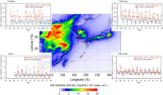
| Yokosuka | −0.97 (−5.92%) ** | −0.27 (−2.54%) ** | −1.12 (−4.77%) ** | −1.27 (−4.14%) ** | −0.99 (−4.78%) ** |
| Gwangju | 0.45 (4.54%) ** | 0.04 (0.55%) | 0.39 (4.43%) ** | −0.75 (−5.31%) ** | −0.04 (−0.38%) |
| Fukue | −0.22 (−10.5%) ** | −0.03 (−2.14%) * | 0.00 (−0.22%) | −0.38 (−7.97%) ** | −0.09 (−3.29%) ** |
| Cape Hedo | −0.03 (−3.34%) ** | −0.01 (−1.64%) ** | −0.01 (−0.70%) ** | −0.01 (−1.31%) ** | −0.01 (−1.64%) ** |
| (b) OMI satellite | |||||
| Yokosuka | −0.54 (−4.50%) ** | −0.15 (−2.30%) ** | −0.66 (−4.62%) ** | −0.92 (−4.79%) ** | −0.54 (−4.10%) ** |
| Gwangju | 0.01 (0.16%) | 0.04 (1.41%) ** | −0.01 (−0.22%) | 0.11 (1.65%) ** | 0.03 (0.61%) |
| Fukue | 0.01 (0.59%) + | 0.02 (2.14%) ** | 0.02 (1.22%) + | −0.11 (−4.04%) ** | 0.01 (0.43%) |
| Cape Hedo | 0.04 (3.57%) ** | 0.01 (1.52%) ** | 0.01 (1.12%) ** | 0.00 (0.34%) ** | 0.01 (1.81%) ** |
Publisher’s Note: MDPI stays neutral with regard to jurisdictional claims in published maps and institutional affiliations. |
© 2021 by the authors. Licensee MDPI, Basel, Switzerland. This article is an open access article distributed under the terms and conditions of the Creative Commons Attribution (CC BY) license (https://creativecommons.org/licenses/by/4.0/).
Share and Cite
Choi, Y.; Kanaya, Y.; Takashima, H.; Irie, H.; Park, K.; Chong, J. Long-Term Variation in the Tropospheric Nitrogen Dioxide Vertical Column Density over Korea and Japan from the MAX-DOAS Network, 2007–2017. Remote Sens. 2021, 13, 1937. https://doi.org/10.3390/rs13101937
Choi Y, Kanaya Y, Takashima H, Irie H, Park K, Chong J. Long-Term Variation in the Tropospheric Nitrogen Dioxide Vertical Column Density over Korea and Japan from the MAX-DOAS Network, 2007–2017. Remote Sensing. 2021; 13(10):1937. https://doi.org/10.3390/rs13101937
Chicago/Turabian StyleChoi, Yongjoo, Yugo Kanaya, Hisahiro Takashima, Hitoshi Irie, Kihong Park, and Jihyo Chong. 2021. "Long-Term Variation in the Tropospheric Nitrogen Dioxide Vertical Column Density over Korea and Japan from the MAX-DOAS Network, 2007–2017" Remote Sensing 13, no. 10: 1937. https://doi.org/10.3390/rs13101937
APA StyleChoi, Y., Kanaya, Y., Takashima, H., Irie, H., Park, K., & Chong, J. (2021). Long-Term Variation in the Tropospheric Nitrogen Dioxide Vertical Column Density over Korea and Japan from the MAX-DOAS Network, 2007–2017. Remote Sensing, 13(10), 1937. https://doi.org/10.3390/rs13101937