Article

Using Landsat Imagery to Assess Burn Severity of National Forest Inventory Plots

1
Department of Forest Resources Management, The University of British Columbia, 2424 Main Mall, Vancouver, BC V6T 1Z4, Canada
2
Corvallis Forestry Sciences Laboratory, Pacific Northwest Research Station, USDA Forest Service, 3200 SW Jefferson Way, Corvallis, OR 97331, USA
*
Author to whom correspondence should be addressed.
Remote Sens. 2021, 13(10), 1935; https://doi.org/10.3390/rs13101935
Submission received: 29 March 2021 / Revised: 1 May 2021 / Accepted: 6 May 2021 / Published: 15 May 2021
(This article belongs to the Section Forest Remote Sensing)

Abstract

:
As the frequency and size of wildfires increase, accurate assessment of burn severity is essential for understanding fire effects and evaluating post-fire vegetation impacts. Remotely-sensed imagery allows for rapid assessment of burn severity, but it also needs to be field validated. Permanent forest inventory plots can provide burn severity information for the field validation of remotely-sensed burn severity metrics, although there is often a mismatch between the size and shape of the inventory plot and the resolution of the rasterized images. For this study, we used two distinct datasets: (1) ground-based inventory data from the United States national forest inventory to calculate ground-based burn severity; and (2) remotely-sensed data from the Monitoring Trends in Burn Severity (MTBS) database to calculate different remotely-sensed burn severity metrics based on six weighting scenarios. Our goals were to test which MTBS metric would best align with the burn severity of national inventory plots observed on the ground, and to identify the superior weighting scenarios to extract pixel values from a raster image in order to match burn severity of the national inventory plots. We fitted logistic and ordinal regression models to predict the ground-based burn severity from the remotely-sensed burn severity averaged from six weighting scenarios. Among the weighting scenarios, two scenarios assigned weights to pixels based on the area of a pixel that intersected any parts of a national inventory plot. Based on our analysis, 9-pixel weighted averages of the Relative differenced Normalized Burn Ratio (RdNBR) values best predicted the ground-based burn severity of national inventory plots. Finally, the pixel specific weights that we present can be used to link other Landsat-derived remote sensing metrics with United States forest inventory plots.

1. Introduction

Wildfires shape the structure and composition of forests from local sites to the global landscape across a wide range of ecosystems [1]. With the changing climate, the length of wildfire seasons has increased [2], while fires have become more frequent and larger in size [3,4,5]. To support planning before and during fires and to assist post-fire recovery, the collection of field and remotely-sensed data on fire and burn severity is critical [6,7]. Burn severity data are also essential for monitoring post-fire recovery for carbon accounting purposes [8], and for assessing the probability of reburns across fire severity classes [9]. We use the term burn severity here to describe the longer-term ecological impacts of fire on vegetation and soils [10,11,12,13].
At the landscape level, satellite imagery has been critical to quickly assess burn severity at low costs, while reducing the need for more time consuming and possibly dangerous field sampling [13]. Multiple remotely-sensed metrics have been developed to quantify burn severity by measuring the post-fire magnitude of vegetation change based on satellite images. The basis of many remotely-sensed metrics is a spectral index called Normalized Burn Ratio (NBR), which is based on bands 4 and 7 of the Landsat Thematic Mapper (TM) or Enhanced Thematic Mapper Plus (ETM+) [10]. The difference between pre- and post-fire metrics can be calculated in absolute terms (differenced NBR; dNBR) [10] or in relative terms (relative differenced Normalized Burn Ratio; RdNBR) [14]. With RdNBR, fires can be compared across time and space, and a single set of thresholds can be used to classify fires in severity categories [14].
In the United States (US or USA), the Monitoring Trends in Burn Severity (MTBS) program uses Landsat-TM imagery to map the perimeter and burn severity of large fires across all types of ownership [15]. A known issue of the MTBS program is that it does not automatically apply an offset to correct dNBR for phenological differences between pre- and post-fire imagery, and the onus is on the user to perform this additional step to normalize dNBR [16]. Another concern, which hinders the needed accuracy to assess burn severity trends and patterns, is the subjectivity of the MTBS analyst that assigns thresholds to place fires in thematic severity classes [16]. However, measures are implemented to ensure consistency in determining burn severity thresholds among analysts [17].
Data collected by the US Forest Inventory and Analysis (FIA) program provide a spatially and temporally balanced sample of forest conditions across all ownerships and forest types in the US [18]. Some permanent FIA plots are burned by wildfires every year [9] and can ultimately be used to field-validate MTBS data at larger scales. However, until now, FIA data have not been widely used to evaluate fire effects (e.g., burn severity) on forests. Additionally, FIA plots and MTBS fire data have seldom been integrated to analyze burn severity. One example is a study by Shaw et al. [19], who integrated both datasets to assess the type of forest cover burned in large fires and the relationship between pre-fire stand conditions and burn severity. Another example is Woo et al. [20], who quantified wildfire effects on forest carbon mass estimated from FIA plots by MTBS severity class.
Although remotely-sensed metrics like the ones provided by the MTBS program are essential to map the burn severity of large areas, they also need to be related to field plots, and be field validated to objective ecological metrics [16,21]. Past studies have examined the errors in registration between the remotely-sensed data and field plots [21,22]. However, an issue that has received little attention is the effect of the mismatch between the size and shape of a field plot and the pixel resolution used to remotely assess the plot condition. For example, an FIA plot only partially overlaps with multiple 30 × 30 m pixels. Several studies have approached the combination of multiple pixels differently, but these combinations have not been compared. Moreover, the issue associated with the effects of the mismatch between the field plots and pixel resolution is not exclusive to the remotely-sensed assessment of burn severity, but rather a concern for any study that uses field plots and remotely-sensed imagery in raster format.
For burn severity assessment, some past techniques to link field plots with remotely-sensed imagery include single-cell intersection [19], 9-pixel averages [14,23,24], and bilinear interpolation [25,26]. Key and Benson [10] have also suggested calculating remotely-sensed burn severity by weighting a five-point pixel average where the centre pixel is counted at least twice. In their scenario, the five points included the plot centre and plus or minus 15 m from the plot centre [10]. The pixels intersecting the outside points were counted once, while the centre pixel was counted twice to provide extra weight [10].
For this research, we used ground data collected by the FIA program in California, USA, and remotely-sensed fire data downloaded from the MTBS database. To predict ground-based burn severity with remotely-sensed severity, we followed Whittier and Gray’s [27] approach to calculate ground-based mortality from the FIA plot data. The study objectives of this paper were threefold: (1) estimate the weights assigned to a pixel for 9-pixel and 25-pixel averages, based on the probabilities of the FIA plot intersecting with a pixel; (2) test which MTBS metric—non-offset adjusted dNBR, offset adjusted dNBR, RdNBR, and MTBS thematic classes—would classify most accurately the burn severity of FIA plots; and (3) identify the best weighting scheme to extract pixel values from the MTBS rasters and to predict burn severity derived from FIA ground data. The overarching goals of the paper were to validate MTBS metrics using FIA plot field data and to identify the MTBS metric and pixel weighting scenario that best represented ground-based burn severity. Therefore, the models presented in this paper provide a validation of the MTBS metrics and their ability to represent ground-based burn severity.
Ultimately, this paper can provide guidance to users looking to assign remotely-sensed burn severity to FIA or other national forest inventory plots. Based on model performance, there is evidence that RdNBR is the best suited remotely-sensed metric to assess burn severity when performing an analysis across multiple fires. Suggestions on the weights that can be used to extract pixels that overlay with FIA plots are also provided for users looking to assess burn severity with remotely-sensed metrics. Based on our results, 9-pixel weighted averages of the RdNBR values best predicted the ground-based burn severity of FIA plots.

2. Methods

2.1. Ground-Based Inventory Data

The data used in this analysis were collected by the Forest Inventory and Analysis (FIA) program overseen by the USDA Forest Service’s Pacific Northwest Research Station and by the Vegetation Mapping and Inventory Program of the USDA Forest Service Region 5 (R5) in California. The FIA program monitors and characterizes the status and trends of US forests across all forest types and ownerships through regular inventories [18]. For this purpose, it has a network of permanent ground plots across all of the USA, where the spatial sampling density is approximately one plot every 24 km2 [18]. A spatially balanced number of FIA plots are revisited each year to record qualitative and quantitative vegetation changes resulting in each plot being remeasured at least once every decade [18]. R5 plots are a spatial intensification (around twice the number) of the FIA plots on lands managed by the USDA Forest Service in selected forest types. The FIA and R5 plots are laid-out and measured in identical fashion [28].
We first selected all FIA plots from CA, USA, that were measured within two years of a wildfire, and that fell within MTBS wildfire perimeters, which includes all fires larger than 4 km2 [15]. Within the sample of burned plots, eight plots were burned twice. If most of the trees within the plot died following the first fire, we kept the plot and tree data only for the first fire and discarded the reburn information. However, if most of the trees had survived after the first fire, the reburn information was kept. If a plot was measured twice in the two years following a fire, the measurement closest to the fire date was retained.
The FIA program defines forest land as land with at least 10 percent canopy cover of any size live tally tree species [29]. However, parts of an FIA plot can fall in water or non-forested land, such as agricultural land. For the analysis, we only included plots that were identified as more than 60% forested as measured in the field and provided by the FIA data [29], because of the challenges associated with mapping sparse vegetation cover. The Landsat bands used to detect vegetation are also influenced by exposed soil, parent substrate and soil water content, making it difficult to map vegetation with sparse cover [30]. For the same reason, we excluded plots with ten or less tallied trees. Additionally, we removed plots where more than 25% of the trees were dead before the fire event.
Each FIA plot consists of four circular plots arranged in a Y-shaped pattern. One circular plot is at the centre, and the other plots are 36.58 m from the centre, at 0, 120 and 240 degrees. The circular plots consist of two nested plots; a subplot with a radius of 7.32 m and a macroplot with a radius of 17.95 m [29]. Data for both plot sizes are collected as part of the inventory in California, USA. Within the subplots, trees with a diameter of at least 12.7 cm are recorded, while trees with a diameter of at least 61 cm are recorded within the macroplots [29]. “Tallied trees” are defined as live and standing dead trees [29]. For our objectives, the relevant tree data variables recorded by the FIA program included the status of the tree (live or dead), the decay class if dead (1 to 5, where 5 is most advanced decay), and the diameter at breast height (dbh). Additionally, at the end of 2006, the FIA program started to record the agent of mortality for individual trees and the approximate year of mortality.
All the plots that were considered for the analysis were measured within two years after a fire. Overall, 446 FIA plots that fell within 164 fires were used in the analysis (Figure 1). The majority of forest fires in California occur in mixed conifer and western oak forest types [9].

2.2. Ground-Based Burn Severity

To classify a tree as killed by fire, we looked at the agent of mortality recorded for most of the trees measured in 2007 and onward. Out of the sample of dead trees, only a small proportion (150 trees) had an agent of mortality other than fire. For the trees that had no agent of mortality, we had to determine whether the tree had been killed by a fire based on common sense criteria. The main criterion was that if the decay class for a tree was 1 or 2, the tree would be classified as having been killed by fire if no other information was available. Because the 446 plots considered were sampled within two years of a fire, a decay class higher than 2 would be unlikely for a tree killed by fire. Additionally, if there was an estimated mortality year without information associated to the agent of mortality, the tree would only be classified as killed by fire if the mortality year and the fire year were the same. It is likely that a small number of the trees with missing information about the agent of mortality were incorrectly identified as having been killed by a fire. Of the trees with a known agent of mortality, around 3% of them were killed by another agent than fire. If the same proportion were applied to the trees with unknown mortality agents, around 60 trees out of 7187 dead trees would be incorrectly classified as having been killed by fire. Incorrectly classified trees would ultimately represent less than 1% of the overall dead trees, which was considered negligible.
Although ground-based burn severity has often been measured based on composite indices like the composite burn index (CBI) [10], they are not ecologically meaningful [13]. For that reason, we chose to measure ground-based burn severity that would reflect actual effects of fire on the vegetation by calculating the percentage of tree mortality.
Based on the density (number of trees per ha) of fire-killed trees per plot, we calculated two types of mortality response variables for our analysis. For the first response, we used Whittier and Gray’s [27] definition of mortality by way of a metric called % Mort Tally. We adapted the equation to subtract the density of tallied trees that were dead before the fire (Equation (1)) We identified trees that were dead before the fire as trees having a decay class of equal or larger to 3 and not having been killed by fire. We calculated % Mort Tally as seen in Equation (1), where the density of tallied mortality trees is only the density of trees killed by a fire. For the second response variable, we then implemented a set of rules, also from Whittier and Gray [27], to assign a severity class to a selected plot based on the % Mort Tally (Table 1) and created a categorical response variable. We calculated this categorical response variable because it is more often used to assess burn severity than a continuous response, and easier to conceptualize.
% Mort Tally = Number of tallied mortality trees Total tally Number of tallied trees dead before fire
With 39 plots, the very low severity class was the least represented, while the low severity class was the one with the highest number of plots (Table 1).

2.3. Remotely-Sensed Burn Severity

Imagery processing and other statistical analysis were performed using the R computing environment, version 3.6.1 [31], with the following additional packages: maptools [32], rgeos [33], rgdal [34], and raster [35].
Wildfire data were downloaded from the MTBS website (https://www.mtbs.gov/direct-download, accessed on 16 June 2020). MTBS uses spectra from Landsat 7 bands 4 (near-infrared) and 7 (short-wave infrared) that have a 30m resolution and respond in opposite directions to changes in plant productivity and soil moisture [36]. The bands are used to calculate the pre-fire and post-fire NBR (Equation (2)) to produce the dNBR [10]. MTBS computes the dNBR (Equation (3)) for each pixel included in a fire perimeter and creates 30 m resolution raster products NBR and dNBR [15]. In addition, MTBS calculates the RdNBR (Equation (4)), a measure that removes pre-fire vegetation biases [14,30]. Additionally, trained image analysts manually select thresholds to create five class thematic burn severity maps that depict burn severity as unburned to low, low, moderate, high, and increased greenness (increased post-fire vegetation) based on their experiences and interpretations of the dNBR and RdNBR data, and the raw satellite imagery [15].
NBR = R 4 R 7 R 4 R 7 1000
dNBR = NBR pre-fire NBR post-fire
RdNBR = dNBR dNBR offset ( NBR pre-fire / 1000 )
MTBS also provides a dNBRoffset value as part of the metadata for each fire that is not automatically applied to the dNBR. We normalized dNBR for each fire following the recommendations of Kolden et al. [16] by using the following:
dNBR adjusted = ( NBR pre-fire NBR post-fire ) dNBR offset
To obtain remotely-sensed burn severity values that could be compared to ground-based burn severity, we extracted the pixel values of the non-offset adjusted dNBR, the RdNBR, and the five-class thematic rasters for a 5 × 5 grid around each FIA plot centre. To assign values of these remotely-sensed metrics to an FIA plot, weighted averages of the remotely-sensed metrics were then calculated based on six scenarios (Table 2). Not all scenarios used the 25 pixels from the 5 × 5 grid but it was convenient to extract them all simultaneously. The first scenario used a single pixel (Figure 2a), scenarios 2, 3, and 4 used weighted averages of 9 pixels (Figure 2b), and scenarios 5 and 6 used weighted averages of 25 pixels (Figure 2c).
For scenarios 4 and 6, the weighted average for the remotely-sensed metrics was based on macroplot pixel specific weights. To assign a weight to a pixel, we calculated the area of a pixel that intersected any parts of the four circular plots that form an FIA plot using a Monte Carlo approach (Figure 2b,c; for more details see Appendix A).
The MTBS thematic classes were treated as a continuous variable ranging from 1 to 4 to calculate the weighted averages for the different scenarios. For every FIA plot, the weighted average for the six scenarios (Table 2) was calculated in terms of non-offset adjusted dNBR, offset adjusted dNBR, RdNBR and MTBS thematic classes.
Finally, we plotted the normalized density of the non-offset adjusted dNBR, offset adjusted dNBR and RdNBR for the different weighting scenarios as smoothed histograms. By looking at the normalized density across the range of values for the different metrics, we were able to observe where the weighting scenarios led to diverging or converging pixel averages. This helped us understand the severity range within which the choice of a pixel scenario made a difference for the individual remotely-sensed metrics. Across the range of remotely-sensed metrics, the normalized density also helped visualized what was going on beyond the confusion matrices resulting from our fitted models.

2.4. Models for Burn Severity Class

To test which remotely-sensed metric and which of the scenarios outlined in Table 2 would best align with observed ground-based burn severity of FIA plots, we used two approaches. The first approach used was logistic regression, where the response variable, % Mort Tally, was treated as a binomial variable. The second approach was ordinal regression, where the response variable, burn severity classes based on % Mort Tally (Table 1), was a categorical variable.
For both types of regression models, we tested four different remotely-sensed metrics as the potential predictor variables. Those metrics were non-offset adjusted dNBR, offset adjusted dNBR, RdNBR, and the MTBS burn severity classes. Using the six different weighting scenarios (Table 2), a total of 24 models—six scenarios for the four remotely-sensed metrics—were compared for each regression type.
Logistic regression with binomial response—The proportion of trees that were killed by a fire per plot (% Mort Tally) were treated as binomial variables with a logit link. Generalized linear models (GLMs; [37]) were fitted with quasi-likelihood to account for overdispersion caused by the lack of independence of trees within a plot. The GLMs were used to test which weighting scenario (Table 2) and remotely-sensed metric would best represent the ground-based burn severity of FIA plots. Model performance was assessed based on the Akaike information criterion (AIC) [38] following Bolker’s [39] recommendations for quasi models in R. Therefore, the AIC was extracted from the logistic regression with binomial response [39]. Model fit was assessed with root mean square predictive error (RMSPE) and prediction bias (e.g., Temesgen et al. [40]).
Ordinal regression with categorical response—For these models, the predictor variables were the weighted remotely-sensed severity metrics, while the response variables were the burn severity classes based on Table 1. For the ordinal regression, we looked at the 24 models as explained above, but we also modelled another set of 24 models where we combined the very low and low severity classes as one class, bringing the number of severity classes from five to four. The MASS [41] and caret [42] R packages were used for the analysis.
To identify the superior model among the six pixel weighting scenarios, we looked at the AIC, the kappa coefficient, and the percentage of correctly classified plots for a model [43]. Kappa is a statistic that indicates the model classification performance relative to the classification expected to occur by chance [44]. The kappa statistic ranges from −1 to +1, where +1 shows perfect agreement, and values below zero show a performance that is no better than random [44]. Past studies have suggested that classification performance assessed through kappa can be broadly classified as slight (0–0.20), fair (0.21–0.4), moderate (0.41–0.60), and substantial (0.61–1) [45,46]. Finally, we calculated the weighted kappa coefficient [47], which considers misclassifications in adjacent classes by assigning a weighted penalty proportional to the squared distance to the correct class.

3. Results

3.1. Macroplot Pixel Specific Weights

The remotely-sensed metrics for scenario 4 were calculated based on a 9-pixel weighted average with macroplot pixel specific weights (Figure 2b), while they were similarly based on a 25-pixel weighted average for scenario 6 (Figure 2c). For scenario 6, based on the average area of the pixels covered by the plot, no part of the FIA plot ever falls in the top two left and right corner pixels. Therefore, the weights assigned to those pixels were zero (Figure 2c).

3.2. Smoothed Histograms of the Remotely-Sensed Metrics

First, for the three remotely-sensed metrics we observed—non-offset adjusted dNBR, offset adjusted dNBR, and RdNBR—three of the five plotted weighting scenarios, scenario 2 (9 pixels with equal weights), scenario 4 (9 pixels with macroplot pixel specific weights), and scenario 6 (25 pixels with macroplot pixel specific weights), all had smoothed histogram that closely followed one another across the range of values that was plotted (Figure 3).
Another common pattern among the three remotely-sensed metrics emerged, which was that the distribution of the metrics was skewed to the left for all weighting scenarios. However, the smoothed histogram for the 1-pixel scenario was slightly more left skewed (i.e., the peak happened earlier) than other scenarios and had slightly greater variability (i.e., the peak is lower and the histogram more spread). This was expected for the 1-pixel scenario compared to the other scenarios that were averages and, therefore, less variable. In comparison, the 25-pixel equal weights scenario was not displaced as much to the left as the 1-pixel scenario. The 25-pixel equal weights scenario had less variability than other scenarios (i.e., higher peak), which was expected as we averaged a higher number of pixels for this scenario. Finally, at both the lower and upper tails, the five weighting scenarios converged for the three remotely-sensed metrics (Figure 3).
Despite common patterns, the overall appearance of the smoothed histograms was not consistent across all three remotely-sensed metrics. For the non-offset adjusted (Figure 3a) and the offset adjusted dNBR (Figure 3b), the normalized density across all five scenarios closely resembled one another. The similarities between the non-offset adjusted and offset adjusted dNBR were expected as the offset is the only difference between the two metrics and is often small. Finally, the left skew was less noticeable for the RdNBR (Figure 3c) compared to the previous two metrics, and the histogram for RdNBR was flatter, denoting more variability. The spread across the range of values for RdNBR could have been evidence of the metrics’ ability to better discriminate along the range of severity.

3.3. Logistic Regression

With lower AIC ranging from 3886.89 to 4362.60, the RdNBR models performed consistently better at representing ground-based severity than the non-offset adjusted dNBR (AIC: 4552.91 to 5161.84), the offset adjusted dNBR (AIC: 4461.40 to 5029.62), and the thematic MTBS severity classes (AIC: 5040.03 to 5419.54; Appendix B, Table A1, Table A2 and Table A3). Based on the AIC, the thematic MTBS classes performed the worst as a predictor of the ground-based severity with the highest AIC values. Based on the AIC values, the offset adjusted dNBR models performed slightly better than the non-offset adjusted dNBR models.
With the lowest AIC value, scenario 4, which is the 9-pixel weighted average based on macroplot specific weights, was slightly superior than other RdNBR models in representing ground-based burn severity (Table 3). However, scenario 3, was very similar to scenario 4 in terms of model performance with a ΔAIC of 6.80, which shows no substantial difference between the two models [48]. Of the six logistic models for RdNBR, the equally-weighted average of 25 pixels around the plot centre (scenario 5) had the highest AIC and performed the worst to predict ground-based burn severity of FIAplots (Table 3). Scenario 1, using a single-pixel RdNBR value, was also an inferior model because it had a much higher AIC than scenarios 2, 3, 4, and 6 (Table 3).
RMSPE tended to be smallest for the 9-pixel weighted average based on macroplot specific weights and the 9-pixel averages with the centre pixel counted twice. RMSPE was smallest for models using RdNBR and largest for models using the thematic MTBS classes as predictor variables, suggesting that the RdNBR models achieved the best model fit across the four remotely-sensed metrics. The prediction bias was negligible (Table 3; Appendix B, Table A1, Table A2 and Table A3) and tended to be smallest for the 9-pixel averages.

3.4. Ordinal Regression

3.4.1. General Relationships

The four remotely-sensed metrics were plotted against the categorical FIA plot ground-based burn severity (Figure 4). The general pattern that emerged was that the values for remotely-sensed metrics were very similar for the very low and low ground-based burn severity, which affected the overall classification accuracy once the remotely-sensed and ground-based burn severity were modelled. In general, the remotely-sensed values did not overlap as much across classes for the three higher ground-based severity classes (Figure 4). Finally, when the MTBS thematic class values were plotted against ground-based burn severity, the values across classes overlapped more than for the other remotely-sensed metrics (Figure 4d).

3.4.2. Model Fitting

Due to the considerable overlap between the very low and low severity classes (Figure 4), the ordinal regression models with five ground severity classes in the response did not perform as well to predict ground-based severity as the models where the severity classes very low and low were combined. With five ground-based severity classes, the AIC of the RdNBR models ranged from 897.04 to 947.85 (Appendix B, Table A7), while they ranged from 701.66 to 745.93 with four ground-based severity classes (Table 4). Therefore, the focus will remain on the four-class models for the remainder of the section.
As observed for the logistic regression models, the RdNBR was a better predictor for four class ground-based burn severity in the ordinal regression models than the other remotely-sensed metrics, with a lower range of AIC values (see Appendix B, Table A4, Table A5 and Table A6). Compared to the AIC values mentioned above for RdNBR (Table 4), the AIC for the non-offset adjusted dNBR models ranged from 785.42 to 832.57, from 782.62 to 827.99 for the offset adjusted dNBR models, and from 815.59 to 870.74 for the thematic MTBS class models. The thematic MTBS classes again performed the worst to predict ground-based mortality based on the AIC values. For both dNBR metrics, the performance of the models were similar based on similar AIC ranges.
For the RdNBR metric, the models of scenarios 2, 3, 4 and 6 showed no substantial differences with a ΔAIC of 2.81 (Table 4) among the four models [48]. The 1-pixel and 25 pixels equally-weighted average models both resulted in AIC values higher than the other scenarios, and therefore did not perform as well in representing the ground-based burn severity classes based on RdNBR (Table 4).

3.4.3. Classification

Based on the kappa coefficient, the classification performance of all the RdNBR models could be described as moderate, because the kappa values fell within the 0.41–0.60 interval (Table 4). Similarly as with the AIC, the kappa (0.50–0.51), weighted kappa (0.70) and percentage of correctly classified plots were very similar (65%–66%) among scenarios 2, 3, 4, and 6 (Table 4). More specifically, the overall classification accuracy was 66% for scenarios 3 and 65% for scenario 4 (Table 4), and the confusion matrices confirmed that both models performed very similarly in the classification of ground-based burn severity (Table 5 and Table 6).
Based on the confusion matrices, the classification accuracy was best for the very low\low severity class with above 81% of the plots correctly classified for both models (Table 5 and Table 6). The classification accuracy was also high for the severe ground-based class with 80% and 78.9% of plots correctly classified, respectively, for scenarios 3 and 4. The classification accuracy was much lower for the moderate and moderately severe classes for both scenarios. However, many of the misclassifications that occurred were in adjacent severity classes. The weighted kappa value, which considers misclassifications in adjacent classes, was 0.70 for both scenarios 3 and scenario 4 (Table 4). These weighted kappa values showed that the overall classification performance was substantial for both scenarios. Given all fit statistics calculated, the RdNBR model for scenario 3, where the weighted average was calculated from 9 pixels with the centre pixel counted twice, could be considered the best model in contrast with the other scenarios.
In contrast with the best performing RdNBR ordinal regression models, the overall classification accuracy for scenario 4 of the offset adjusted dNBR model was 61%, and the kappa statistic was 0.43 (Appendix B, Table A5). The main difference between the confusion matrices of the RdNBR model (Table 6) and the offset adjusted dNBR model (Table 7) was the ability of the RdNBR model to accurately predict that a plot would fall in the moderately severe class. The RdNBR scenario 4 model (Table 6) had a classification accuracy for the moderately severe class of 31.1% versus 13.1% for the dNBR scenario 4 model (Table 7). For the three other severity classes, the classification accuracy was comparable for the RdNBR and dNBR models (Table 6 and Table 7).

4. Discussion

4.1. Remotely-Sensed Metrics

One objective of this paper was to test which MTBS remotely-sensed metric would be best to predict the observed ground-based burn severity of FIA plots. The four metrics used were non-offset adjusted dNBR, and offset adjusted dNBR, which are both measures of the absolute change in Landsat’s bands; RdNBR, which measures relative changes in bands; and thematic MTBS severity classes assigned by an MTBS analyst. The models that were fitted and the statistical comparison showed that RdNBR was best in terms of AIC at representing the ground-based severity of FIA plots, both when the ground-based severity was treated as a binomial and a categorical response variable.
Past studies have shown mixed results in terms of overall classification accuracy between dNBR and RdNBR. Miller et al. [30] showed that the classification accuracy across all levels of severity classes was not better for RdNBR compared to dNBR, but that the classification accuracy for high burn severity was higher with RdNBR in the conifer dominated Sierra Nevada and Klamath Mountains, USA. In contrast, Soverel et al. [22] found that dNBR had higher classification accuracy than RdNBR in the Canadian boreal forest and the Canadian Rockies, while Hudak et al. [49] found that RdNBR was not more appropriate than dNBR to assess immediate post-fire burn severity on plots in Alaska, Montana, and California, USA. Finally, Cansler and McKenzie [25] found no significant difference in the overall classification accuracy between dNBR and RdNBR in the Cascade Range, USA. Because RdNBR was intended for locations where pre-fire reflectance is variable [14], it possibly performed better in this study across California, where the vegetation is diverse, compared to more northern locations like the boreal forest [22] where the pre-fire vegetation cover is more constant and homogeneous. Additionally, the important difference (18%) in classification accuracy between RdNBR scenario 4 (Table 6) and offset adjusted dNBR scenario 4 (Table 7) for the moderately severe class confirmed Miller et al.’s [30] results that RdNBR performs better than dNBR to classify higher burn severity.
To note here is that the choice of our ground-based severity measure, % Mort Tally, and subsequent categorization in severity classes (Table 1), was intentional as we wanted to record actual fire effects on vegetation, which in this case was the percentage tree mortality as suggested by Morgan et al. [13]. However, this approach differed from many of the studies mentioned above that used composite metrics such as the composite burn index (CBI) or similar indices to asses ground-based burn severity [21,22,49]. Miller et al. [30] was the only study that used percentage tree mortality in addition to CBI to measure ground-based burn severity. In contrast with Miller et al. [30], our results showed that RdNBR was more accurately representing the ground-based burn severity than dNBR across all levels of severity classes.
Although RdNBR performed best to predict ground-based burn severity, there are also some issues associated with this metric [26]. For example, the RdNBR denominator can be zero if the NBR pre-fire is zero, which would result in an undefined RdNBR that cannot be interpreted or compared with other values [26]. To avoid the issues associated with RdNBR, Parks et al. [26] introduced the Relativized Burn Ratio (RBR) where 1.001 is added to the NBR pre-fire to form the denominator. As of now, RBR is not a product of the MTBS database, but could be added in the future, and it should also be compared with the metrics we used in our analysis.
Moreover, the statistical comparison showed that the models using the MTBS thematic severity classes as the predictor variable performed the worst at representing ground-based burn severity compared to the other remotely-sensed metrics. Because the thematic classes are the results of forcing continuous data into a restricted number of categories, some nuances in the data may have been lost, which reduced the predictive abilities [50]. Additionally, the thresholds used to categorize burn severity are subjective and not field validated to objective ecological metrics [16], which can lead to misclassified plots. Misclassifications of thematic MTBS classes have been reported by other studies such as Shaw et al. [19] that used single-cell intersections of MTBS thematic classes.
Regarding the results for the two dNBR models, the offset adjusted dNBR models performed slightly better than the non-offset adjusted dNBR. The dNBR offset has rarely been the focus of research, and statistical comparisons on the effect of the offset are sparse. Nonetheless, the offset can be important when comparing dNBR among fires that have natural phenological differences [36]. In their paper, Kolden et al. [16] emphasized the need to apply the offset to dNBR values extracted from the MTBS database. However, our analysis, which was performed across 164 fires, showed that the subtraction of the offset, when comparing multiple fires, might not be critical, because both approaches led to very similar results.

4.2. Pixel Configuration and Weighting

Another objective of this paper was to compare weighting scenarios for the remotely-sensed severity metrics to identify which scheme would align most closely with the FIA plot ground-based severity. We modelled 6 scenarios for each of the four remotely-sensed severity metrics for the two modelling approaches: logistic regression and ordinal regression. The scenario that was consistently inferior was the 25-pixel equally-weighted average. This was most likely due to the inclusion of pixels that do not overlap the FIA plot. Fires do not burn heterogeneously across a landscape, and the burn severity may therefore vary spatially [13]. Mixed severity fires are also typical of much of the mixed conifer forest in California [51]. Twenty-five pixels represent a large ground area, and it is reasonable to assume that varying severity across space would create a heterogeneous mix of patches resulting in fluctuating remotely-sensed metrics. These results are analogous to Key and Benson’s [10] findings that a 9-pixel average did not overlap with the severity of a 30 m diameter plot. Additionally, when multiple pixels are averaged, the variability is reduced, which leads to less extreme values and more plots in the moderate burn severity range that become challenging to accurately predict as shown in the confusion matrices (Table 5, Table 6 and Table 7).
The results for the 1-pixel configuration were mixed depending on the regression type. For the logistic regression, across remotely-sensed metrics, the 1-pixel models did not perform as well compared to other scenarios. However, for the ordinal regression, the RdNBR 1-pixel scenario performed similarly to the best models in terms of Kappa statistics and percentage of correctly classified plots although it had a higher AIC (Table 4). The improvement of the 1-pixel scenario when the response variable was categorical could be explained by the loss of information that occurs when continuous variables are binned. Therefore, there is evidence that the 1-pixel scenario performed well to predict the four class categorical ground-based burn severity response that had lost nuances in the binning process.
Classifying plots with partial mortality is a known shortcoming of imagery-based interpretations [43,52] that our models could not overcome. Our models struggled with the classification of FIA plots that were labelled as moderate and moderately severe based on the observed ground-based burn severity (Table 5, Table 6 and Table 7). In general, the accurate classification of moderately severe burn areas could be harder due to the larger variation in pixel values that represent such area. That said, the choice of a weighting scenario is of higher importance within the moderate burn severity range where the remotely-sensed metrics based on 1 pixel or 25 equally weighted pixels diverged from other scenarios. At the tails, for very low\low and severe burn severity, the weighting scenario chosen does not have as much of an impact on classification because all scenarios converged to yield similar results (Figure 3).
Across remotely-sensed metrics for the logistic regression, the three scenarios that used different weighted averages of 9 pixels performed similarly in representing ground-based severity. However, the model with the weighted average based on the macroplot pixel specific weights performed slightly better with a lower AIC (Table 3). As this scenario best represented the overlap between the pixels and an FIA plot, it is logical that it would perform better than other scenarios. Moreover, the scenario that used an average of the 9 pixels with the centre pixel counted twice, as suggested by Key and Benson [10], performed best to predict ground-based burn severity based on the ordinal regression models. However, also considering the minimal differences in AIC, kappa and classification accuracy among models for scenarios 2, 3, and 4, we concluded that there is no difference among these three models in terms of their classification accuracy. In the end, the choice of a weighting scenario lies with the user, and the complexity they want to add to the pixel extraction process. Because all three scenarios using 9-pixel averages performed similarly both with logistic and ordinal regression, we suggest the use of an equally-weighted average of 9 pixels for simplicity. However, to have the best prediction of the ground-based burn severity based on a remotely-sensed metric, we suggest using the 9-pixel weighted average calculated with the macroplot pixel specific weights, which is the scenario that performed best in terms of the AIC for the logistic regression when the response variable was binomial. Ultimately, having a binomial burn severity response to predict ground-based severity is more valuable than having a categorical response that leads to a loss of information due to data binning.

5. Conclusions

The analysis showed that RdNBR was better than non-offset adjusted dNBR, offset adjusted dNBR and MTBS thematic classes at representing ground-based burn severity of 446 national forest inventory plots across 164 fires in California, USA. We also concluded that to predict the ground-based burn severity of FIA plots, any of the 9-pixel scenarios presented would yield similar results. However, we recommend the use of a 9-pixel average where the weights are proportional to the average area of the pixels covered by the plot to best predict the ground-based burn severity following the results of logistic regression. FIA plots and the MTBS database are commonly used tools, but they have rarely been integrated to provide novel insights on the effects of fires on forests. The large-scale integration of FIA plots and the MTBS database could ultimately improve the latter by allowing for the field validation of classification thresholds.
Applications for the pixel specific proportional weights for calculating weighted averages of remotely-sensed metrics go beyond the assessment of burn severity. The weights, proportional to the average area of the pixels covered by the plot calculated as part of this paper, could be used to extract other remotely-sensed metrics, represented by 30 m rasters, to link to FIA plot data. For example, the pixel specific weights could possibly be used to calculate weighted averages of the Normalized Difference Vegetation Index (NDVI) or the tasseled cap transformations that are both based on Landsat data [53]. These are just two examples of remote sensing metrics among many that use Landsat, and that could be averaged using the pixel weights provided by this study.
Finally, the approach we used to calculate pixel specific weights (Appendix A) could be applied to a range of other plot configurations aside from FIA plots. Pixel weights could be calculated based on the average area of the pixels covered by other types of national forest inventory plots outside the US, and used by forest managers to remotely assess ground variables based on satellite imagery.

Author Contributions

Conceptualization, F.P., B.N.I.E., and V.J.M.; Methodology, F.P., B.N.I.E., and V.J.M.; Software, F.P., B.N.I.E., V.J.M., and Y.-C.T.; Formal analysis and investigation, F.P., B.N.I.E., and V.J.M.; Resources, B.N.I.E. and V.J.M.; Data curation, F.P. and V.J.M.; Writing—original draft preparation, F.P.; Writing—review and editing, B.N.I.E., V.J.M., and Y.-C.T.; Visualization, F.P. and Y.-C.T.; Supervision, B.N.I.E. and V.J.M.; Project administration and funding acquisition, B.N.I.E. and V.J.M. All authors have read and agreed to the published version of the manuscript.

Funding

This research was funded by the USDA Forest Service Pacific Northwest (PNW) Research Station through agreement 14-JV-11261959–069 and an NSERC Discovery Grant held by Bianca Eskelson. The project was further supported by the University of British Columbia Work Learn program student salary subsidy.

Acknowledgments

We would like to thank Nicholas Coops for his feedback and comments at multiple steps of this project. Additionally, we would like to thank the reviewers for their constructive feedback. We also thank the many individuals involved in the design, field data collection, quality assurance, and processing of the U.S. Forest Service Forest Inventory and Analysis Program.

Conflicts of Interest

The authors declare no conflict of interest.

Appendix A. Pixel Weight Calculation

To estimate the weights assigned to each pixel, we calculated the area of a pixel that intersected any parts of the four circular plots that form an FIA plot. Because there is uncertainty regarding the position of the FIA plot centre within the centre pixel, and due to fact that the position of the FIA plot centre differs for each plot, we calculated the average intersected area for all possible locations of the plot centre within the centre pixel. To do so, we superposed a 1m by 1m grid across the centre pixel (961 points), centered the centre plot at each of those points, and estimated the area of intersection between the FIA plot and the pixel. For each of the points in the centre pixel, the intersection area was estimated using a Monte Carlo approach with 10 million points. Finally, the intersection areas were normalized to add to 1, and averaged over the 961 points. These areas calculated for each pixel were the weights used in scenario 4 and 6 of our analysis.
For west coast states, including California, the four circular plots that are part of an FIA plot are composed of a subplot and a macroplot while the FIA plots in the rest of the US only have subplots (Figure A1a). The same approach was used to calculate the weights for both the macroplots and the subplots. The weights for the macroplots are displayed in Figure 2 in the methodssection, while the weights that should be used to calculate a weighted average with subplots for remotely-sensed metrics are available below (Figure A1b,c).
Figure A1. (a) Example of an FIA plot, with the four circular plots composed of a macroplot and a subplot, where the plot centre falls exactly in the centre of of the centre pixel; subplots pixel weights to calculate the remotely-sensed metrics for (b) 9 pixels (scenario 4) and (c) 25 pixels (scenario 6).
Remotesensing 13 01935 g0a1

Appendix B. Model Comparisons

Appendix B.1. Logistic Regression

Table A1. Non-offset adjusted dNBR—AIC, ΔAIC, RMSPE and bias for the logistic regression with non-offset adjusted dNBR to predict the ground-based severity expressed as % Mort Tally. The scenario with a ΔAIC of 0 has the lowest AIC.
ScenarioDescriptionAICΔAICRMSPEBias
11 pixel4761.65207.730.220−0.003
29 pixels with equal weights4609.4555.540.216−0.002
39 pixels with centre pixel counted twice4586.6332.720.215−0.002
49 pixels with macroplots pixel weights4553.910.000.214−0.002
525 pixels with equal weights5161.84607.920.234−0.001
625 pixels with macroplots pixel weights4610.4256.510.216−0.001
Table A2. Offset adjusted dNBR—AIC, ΔAIC, RMSPE and Bias for the logistic regression with offset adjusted dNBR to predict the ground-based severity expressed as % Mort Tally. The scenario with a ΔAIC of 0 has the lowest AIC.
ScenarioDescriptionAICΔAICRMSPEBias
11 pixel4696.70235.300.218−0.004
29 pixels with equal weights4506.0344.640.213−0.002
39 pixels with centre pixel counted twice4486.6725.270.213−0.002
49 pixels with macroplots pixel weights4461.400.000.211−0.003
525 pixels with equal weights5029.62568.220.231−0.001
625 pixels with macroplots pixel weights4510.4249.030.213−0.002
Table A3. Thematic MTBS classes—AIC, ΔAIC, RMSPE and Bias for the logistic regression with thematic MTBS classes to predict the ground-based severity expressed as % Mort Tally. The scenario with a ΔAIC of 0 has the lowest AIC.
ScenarioDescriptionAICΔAICRMSPEBias
11 pixel5671.11631.080.244−0.003
29 pixels with equal weights5040.030.000.2260.000
39 pixels with centre pixel counted twice5045.735.700.2260.000
49 pixels with macroplots pixel weights5056.9116.880.2260.000
525 pixels with equal weights5419.54379.510.2400.002
625 pixels with macroplots pixel weights5060.2320.200.2270.001

Appendix B.2. Ordinal Regression

Appendix B.2.1. Model Comparisons for 4-Classes Ground-Based Severity Models

Table A4. Non-offset adjusted dNBR—Fit statistics for the ordinal regression using non-offset adjusted dNBR as the predictor variable and 4-class ground-based severity as the response variable. The scenario with a ΔAIC of 0 has the lowest AIC.
ScenarioDescriptionAICΔAICKappaWeighted% Correctly
KappaClassified
11 pixel801.8816.460.440.6262%
29 pixels with equal weights788.993.570.450.6362%
39 pixels with centre pixel counted twice786.941.520.440.6362%
49 pixels with macroplots pixel weights785.420.000.460.6463%
525 pixels with equal weights832.5747.150.410.6060%
625 pixels with macroplots pixel weights789.744.320.440.6261%
Table A5. Offset adjusted dNBR—Fit statistics for the ordinal regression using offset adjusted dNBR as the predictor variable and 4-class ground-based severity as the response variable. The scenario with a ΔAIC of 0 has the lowest AIC.
ScenarioDescriptionAICΔAICKappaWeighted Kappa% Correctly Classified
11 pixel801.5518.930.450.6262%
29 pixels with equal weights785.623.000.430.6361%
39 pixels with centre pixel counted twice783.801.180.420.6360%
49 pixels with macroplots pixel weights782.620.000.430.6361%
525 pixels with equal weights827.9945.370.390.5959%
625 pixels with macroplots pixel weights786.353.730.430.6461%
Table A6. Thematic MTBS classes—Fit statistics for the ordinal regression using the thematic MTBS classes as the predictor variable and 4-class ground-based severity as the response variable. The scenario with a ΔAIC of 0 has the lowest AIC.
ScenarioDescriptionAICΔAICKappaWeighted Kappa% Correctly Classified
11 pixel870.7455.150.380.5658%
29 pixels with equal weights815.590.000.410.6059%
39 pixels with centre pixel counted twice815.960.370.390.5958%
49 pixels with macroplots pixel weights817.602.010.380.5858%
525 pixels with equal weights847.0531.460.360.5656%
625 pixels with macroplots pixel weights818.152.560.400.5959%

Appendix B.2.2. Model Comparisons for 5-Classes Ground-Based Severity Models

Table A7. RdNBR—Fit statistics for the ordinal regression using RdNBR as the predictor variable and 5-class ground-based severity as the response variable. The scenario with a ΔAIC of 0 has the lowest AIC.
ScenarioDescriptionAICΔAICKappaWeighted Kappa% Correctly Classified
11 pixel925.0828.040.410.6457%
29 pixels with equal weights898.571.530.420.6557%
39 pixels with centre pixel counted twice897.04hl0.000.420.6557%
49 pixels with macroplots pixel weights897.550.510.420.6557%
525 pixels with equal weights947.8550.810.380.6254%
625 pixels with macroplots pixel weights900.503.460.440.6558%
Table A8. RdNBR confusion matrix for scenario 3 where the remotely-sensed metric is calculated as the equally-weighted average of 9 pixels, and the ground-based burn severity has 5 classes.
Predicted Ground Burn SeverityActual Ground Burn Severity
Very LowLowModerateModerately SevereSevere
Very Low2.6%2.0%1.0%0%0%
Low79.5%75.0%41.7%3.3%1.1%
Moderate18.0%21.6%45.6%34.4%6.3%
Moderately Severe0%0.7%7.8%31.1%12.6%
Severe0%0.7%3.9%31.1%80.0%
Table A9. Offset adjusted dNBR confusion matrix for scenario 4 where the remotely-sensed metric is calculated as the weighted average of 9 pixels based on macroplot pixel specific weights, and the ground-based burn severity has 4 classes.
Predicted Ground Burn SeverityActual Ground Burn Severity
Very LowLowModerateModerately SevereSevere
Very Low0%0.7%1.0%0%0%
Low87.2%81.8%43.7%4.9%1.1%
Moderate10.3%15.5%39.8%47.5%15.8%
Moderately Severe0%1.4%6.8%6.6%7.4%
Severe2.6%0.7%8.7%41.0%75.8%

References

  1. Bowman, D.M.; Balch, J.K.; Artaxo, P.; Bond, W.J.; Carlson, J.M.; Cochrane, M.A.; D’Antonio, C.M.; DeFries, R.S.; Doyle, J.C.; Harrison, S.P.; et al. Fire in the Earth system. Science 2009, 324, 481–484. [Google Scholar] [CrossRef] [PubMed]
  2. Jolly, W.M.; Cochrane, M.A.; Freeborn, P.H.; Holden, Z.A.; Brown, T.J.; Williamson, G.J.; Bowman, D.M. Climate-induced variations in global wildfire danger from 1979 to 2013. Nat. Commun. 2015, 6, 7537. [Google Scholar] [CrossRef] [PubMed]
  3. Dennison, P.E.; Brewer, S.C.; Arnold, J.D.; Moritz, M.A. Large wildfire trends in the western United States, 1984–2011. Geophys. Res. Lett. 2014, 41, 2928–2933. [Google Scholar] [CrossRef]
  4. Miller, J.D.; Skinner, C.; Safford, H.; Knapp, E.E.; Ramirez, C. Trends and causes of severity, size, and number of fires in northwestern California, USA. Ecol. Appl. 2012, 22, 184–203. [Google Scholar] [CrossRef] [PubMed]
  5. Westerling, A.L.; Hidalgo, H.G.; Cayan, D.R.; Swetnam, T.W. Warming and earlier spring increase western US forest wildfire activity. Science 2006, 313, 940–943. [Google Scholar] [CrossRef] [PubMed] [Green Version]
  6. Beschta, R.L.; Rhodes, J.J.; Kauffman, J.B.; Gresswell, R.E.; Minshall, G.W.; Karr, J.R.; Perry, D.A.; Hauer, F.R.; Frissell, C.A. Postfire management on forested public lands of the western United States. Conserv. Biol. 2004, 18, 957–967. [Google Scholar] [CrossRef]
  7. Kuenzi, A.M.; Fulé, P.Z.; Sieg, C.H. Effects of fire severity and pre-fire stand treatment on plant community recovery after a large wildfire. For. Ecol. Manag. 2008, 255, 855–865. [Google Scholar] [CrossRef]
  8. Keith, H.; Lindenmayer, D.B.; Mackey, B.G.; Blair, D.; Carter, L.; McBurney, L.; Okada, S.; Konishi-Nagano, T. Accounting for biomass carbon stock change due to wildfire in temperate forest landscapes in Australia. PLoS ONE 2014, 9, e107126. [Google Scholar] [CrossRef] [Green Version]
  9. Eskelson, B.N.; Monleon, V.J.; Fried, J.S. A 6 year longitudinal study of post-fire woody carbon dynamics in California’s forests. Can. J. For. Res. 2016, 46, 610–620. [Google Scholar] [CrossRef]
  10. Key, C.H.; Benson, N.C. Landscape Assessment (LA). In FIREMON: Fire Effects Monitoring and Inventory System; Lutes, D.C., Keane, R.E., Caratti, J.F., Key, C.H., Benson, N.C., Sutherland, S., Gangi, L.J., Eds.; Gen. Tech. Rep. RMRS-GTR-164-CD; USDA Forest Service, Rocky Mountain Research Station: Fort Collins, CO, USA, 2006; p. 51. [Google Scholar]
  11. Lentile, L.B.; Holden, Z.A.; Smith, A.M.; Falkowski, M.J.; Hudak, A.T.; Morgan, P.; Lewis, S.A.; Gessler, P.E.; Benson, N.C. Remote sensing techniques to assess active fire characteristics and post-fire effects. Int. J. Wildland Fire 2006, 15, 319–345. [Google Scholar] [CrossRef]
  12. French, N.H.; Kasischke, E.S.; Hall, R.J.; Murphy, K.A.; Verbyla, D.L.; Hoy, E.E.; Allen, J.L. Using Landsat data to assess fire and burn severity in the North American boreal forest region: An overview and summary of results. Int. J. Wildland Fire 2008, 17, 443–462. [Google Scholar] [CrossRef]
  13. Morgan, P.; Keane, R.E.; Dillon, G.K.; Jain, T.B.; Hudak, A.T.; Karau, E.C.; Sikkink, P.G.; Holden, Z.A.; Strand, E.K. Challenges of assessing fire and burn severity using field measures, remote sensing and modelling. Int. J. Wildland Fire 2014, 23, 1045–1060. [Google Scholar] [CrossRef] [Green Version]
  14. Miller, J.D.; Thode, A.E. Quantifying burn severity in a heterogeneous landscape with a relative version of the delta Normalized Burn Ratio (dNBR). Remote Sens. Environ. 2007, 109, 66–80. [Google Scholar] [CrossRef]
  15. Eidenshink, J.; Schwind, B.; Brewer, K.; Zhu, Z.L.; Quayle, B.; Howard, S. A project for monitoring trends in burn severity. Fire Ecol. 2007, 3, 3–21. [Google Scholar] [CrossRef]
  16. Kolden, C.A.; Smith, A.M.; Abatzoglou, J.T. Limitations and utilisation of Monitoring Trends in Burn Severity products for assessing wildfire severity in the USA. Int. J. Wildland Fire 2015, 24, 1023–1028. [Google Scholar] [CrossRef]
  17. Picotte, J.J.; Bhattarai, K.; Howard, D.; Lecker, J.; Epting, J.; Quayle, B.; Benson, N.; Nelson, K. Changes to the Monitoring Trends in Burn Severity program mapping production procedures and data products. Fire Ecol. 2020, 16, 1–12. [Google Scholar] [CrossRef]
  18. Bechtold, W.A.; Patterson, P.L. The Enhanced Forest Inventory and Analysis Program-National Sampling Design and Estimation Procedures; Technical Report SRS-80; USDA Forest Service, Southern Research Station: Asheville, NC, USA, 2005.
  19. Shaw, J.D.; Goeking, S.A.; Menlove, J.; Werstak, C.E. Assessment of fire effects based on Forest Inventory and Analysis data and a long-term fire mapping data set. J. For. 2017, 115, 258–269. [Google Scholar] [CrossRef] [Green Version]
  20. Woo, H.; Eskelson, B.N.I.; Monleon, V.J. Matching methods to quantify wildfire effects on forest carbon mass in the U.S. Pacific Northwest. Ecol. Appl. 2021, 11, e02283. [Google Scholar]
  21. Cansler, C.A.; McKenzie, D. How robust are burn severity indices when applied in a new region? Evaluation of alternate field-based and remote-sensing methods. Remote Sens. 2012, 4, 456–483. [Google Scholar] [CrossRef] [Green Version]
  22. Soverel, N.O.; Perrakis, D.D.; Coops, N.C. Estimating burn severity from Landsat dNBR and RdNBR indices across western Canada. Remote Sens. Environ. 2010, 114, 1896–1909. [Google Scholar] [CrossRef]
  23. Hall, R.J.; Freeburn, J.T.; De Groot, W.J.; Pritchard, J.M.; Lynham, T.J.; Landry, R. Remote sensing of burn severity: Experience from western Canada boreal fires. Int. J. Wildland Fire 2008, 17, 476–489. [Google Scholar] [CrossRef]
  24. Kolden, C.A.; Lutz, J.A.; Key, C.H.; Kane, J.T.; van Wagtendonk, J.W. Mapped versus actual burned area within wildfire perimeters: Characterizing the unburned. For. Ecol. Manag. 2012, 286, 38–47. [Google Scholar] [CrossRef]
  25. Cansler, C.A. Drivers of Burn Severity in the Northern Cascade Range, Washington, USA. Master’s Thesis, University of Washington, Seattle, WA, USA, 2011. [Google Scholar]
  26. Parks, S.A.; Dillon, G.K.; Miller, C. A new metric for quantifying burn severity: The relativized burn ratio. Remote Sens. 2014, 6, 1827–1844. [Google Scholar] [CrossRef] [Green Version]
  27. Whittier, T.R.; Gray, A.N. Tree mortality based fire severity classification for forest inventories: A Pacific Northwest national forests example. For. Ecol. Manag. 2016, 359, 199–209. [Google Scholar] [CrossRef]
  28. Eskelson, B.N.; Monleon, V.J. Post-fire surface fuel dynamics in California forests across three burn severity classes. Int. J. Wildland Fire 2018, 27, 114–124. [Google Scholar] [CrossRef]
  29. Forest Inventory and Analysis National Core Field Guide Volume I: Field Data Collection Procedures for Phase 2 Plots; Technical Report; USDA Forest Service: North Bend, WA, USA, 2019.
  30. Miller, J.; Safford, H.; Crimmins, M.; Thode, A.E. Quantitative evidence for increasing forest fire severity in the Sierra Nevada and southern Cascade Mountains, California and Nevada, USA. Ecosystems 2009, 12, 16–32. [Google Scholar] [CrossRef]
  31. R Core Team. R: A Language and Environment for Statistical Computing; R Foundation for Statistical Computing: Vienna, Austria, 2019. [Google Scholar]
  32. Bivand, R.; Lewin-Koh, N. Maptools: Tools for Handling Spatial Objects; R Package Version 0.9-9; 2019. [Google Scholar]
  33. Bivand, R.; Rundel, C. Rgeos: Interface to Geometry Engine—Open Source (’GEOS’); R Package Version 0.5-3; 2020. [Google Scholar]
  34. Bivand, R.; Keitt, T.; Rowlingson, B. Rgdal: Bindings for the ’Geospatial’ Data Abstraction Library; R Package Version 1.4-8; 2019. [Google Scholar]
  35. Hijmans, R.J. Raster: Geographic Data Analysis and Modeling; R Package Version 3.0-12; 2020. [Google Scholar]
  36. Key, C.H. Ecological and sampling constraints on defining landscape fire severity. Fire Ecol. 2006, 2, 34–59. [Google Scholar] [CrossRef]
  37. McCullagh, P.; Nelder, J.A. Generalized Linear Models, 2nd ed.; Chapman and Hall/CRC: Boca Raton, FL, USA, 1989. [Google Scholar]
  38. Akaike, H. Information theory and an extension of the maximum likelihood principle. In Selected Papers of Hirotugu Akaike; Springer: New York, NY, USA, 1998; pp. 199–213. [Google Scholar]
  39. Bolker, B. Dealing with quasi-models in R. Compare 2020, 1, 5–452. [Google Scholar]
  40. Temesgen, H.; Monleon, V.; Hann, D. Analysis and comparison of nonlinear tree height prediction strategies for Douglas-fir forests. Can. J. For. Res. 2008, 38, 553–565. [Google Scholar] [CrossRef] [Green Version]
  41. Venables, W.N.; Ripley, B.D. Modern Applied Statistics with S, 4th ed.; Springer: New York, NY, USA, 2002. [Google Scholar]
  42. Kuhn, M. Caret: Classification and Regression Training; R Package Version 6.0-86; 2020. [Google Scholar]
  43. Ferster, C.J.; Eskelson, B.N.; Andison, D.W.; LeMay, V.M. Vegetation Mortality within Natural Wildfire Events in the Western Canadian Boreal Forest: What Burns and Why? Forests 2016, 7, 187. [Google Scholar] [CrossRef] [Green Version]
  44. Cohen, J. A coefficient of agreement for nominal scales. Educ. Psychol. Meas. 1960, 20, 37–46. [Google Scholar] [CrossRef]
  45. Landis, J.R.; Koch, G.G. The measurement of observer agreement for categorical data. Biometrics 1977, 33, 159–174. [Google Scholar] [CrossRef] [Green Version]
  46. Dash, J.P.; Watt, M.S.; Pearse, G.D.; Heaphy, M.; Dungey, H.S. Assessing very high resolution UAV imagery for monitoring forest health during a simulated disease outbreak. ISPRS J. Photogramm. Remote Sens. 2017, 131, 1–14. [Google Scholar] [CrossRef]
  47. Cohen, J. Weighted kappa: Nominal scale agreement provision for scaled disagreement or partial credit. Psychol. Bull. 1968, 70, 213. [Google Scholar] [CrossRef]
  48. Burnham, K.P.; Anderson, D.R. Multimodel inference: Understanding AIC and BIC in model selection. Sociol. Methods Res. 2004, 33, 261–304. [Google Scholar] [CrossRef]
  49. Hudak, A.T.; Morgan, P.; Bobbitt, M.J.; Smith, A.M.; Lewis, S.A.; Lentile, L.B.; Robichaud, P.R.; Clark, J.T.; McKinley, R.A. The relationship of multispectral satellite imagery to immediate fire effects. Fire Ecol. 2007, 3, 64–90. [Google Scholar] [CrossRef]
  50. Harrell, F.E., Jr. Regression Modeling Strategies: With Applications to Linear Models, Logistic and Ordinal Regression, and Survival Analysis; Springer: Berlin/Heisenberg, Germany, 2015. [Google Scholar]
  51. Jain, T.B.; Battaglia, M.A.; Han, H.S.; Graham, R.T.; Keyes, C.R.; Fried, J.S.; Sandquist, J.E. A Comprehensive Guide to Fuel Management Practices for Dry Mixed Conifer Forests in the Northwestern United States; Technical Report RMRS-GTR-292; USDA Forest Service, Rocky Mountain Research Station: North Bend, WA, USA, 2012.
  52. San-Miguel, I.; Andison, D.W.; Coops, N.C.; Rickbeil, G.J. Predicting post-fire canopy mortality in the boreal forest from dNBR derived from time series of Landsat data. Int. J. Wildland Fire 2016, 25, 762–774. [Google Scholar] [CrossRef]
  53. Crist, E.P.; Cicone, R.C. Application of the tasseled cap concept to simulated thematic mapper data. Photogramm. Eng. Remote Sens. 1984, 50, 343–352. [Google Scholar]
Figure 1. Map of California fires sampled that burned from 1999 to 2017 and of the Forest Inventory and Analysis plots used for the analysis.
Remotesensing 13 01935 g001
Figure 2. Pixel configurations for (a) 1 pixel, (b) 9 pixels and (c) 25 pixels. The numbers are the pixel specific weights calculated for macroplots based on the weight calculation (Appendix A) and used to calculate a weighted average for the remotely-sensed metrics (b) 9 pixels (scenario 4) and (c) 25 pixels (scenario 6). In the background, the four macroplots of an FIA plot have a radius of 17.95 m.
Remotesensing 13 01935 g002
Figure 3. Smoothed histogram of three burn severity metrics by weighting scenarios: (a) non-offset adjusted dNBR, (b) offset adjusted dNBR and (c) RdNBR.
Remotesensing 13 01935 g003
Figure 4. Continuous remotely-sensed severity metrics derived from the 9-pixel weighted average based on the macroplot pixel specific weights (scenario 4) per ground-based burn severity classes: (a) Non-offset adjusted dNBR; (b) offset adjusted dNBR; (c) RdNBR; and (d) thematic MTBS severity classes.
Remotesensing 13 01935 g004
Table 1. Set of rules used to assign ground-based severity classes from the ground measured data. The rules were adapted from Whittier and Gray [27].
Severity ClassRuleNumber of Plots
Very LowNo mortality39
Low% Mort Tally < 25148
Moderate% Mort Tally < 60103
Moderately Severe% Mort Tally < 9061
Severe% Mort Tally ≥ 9091
Table 2. Weighting scenarios used to calculate remotely-sensed burned severity for an FIA plot.
ScenarioPixel ConfigurationWeighted Average
11 pixelweight only applied to centre pixel
29 pixelsequal weight (1/9) applied to 9 pixels
39 pixelscentre pixel has twice the weight (2/10) of other 8 pixels (1/10)
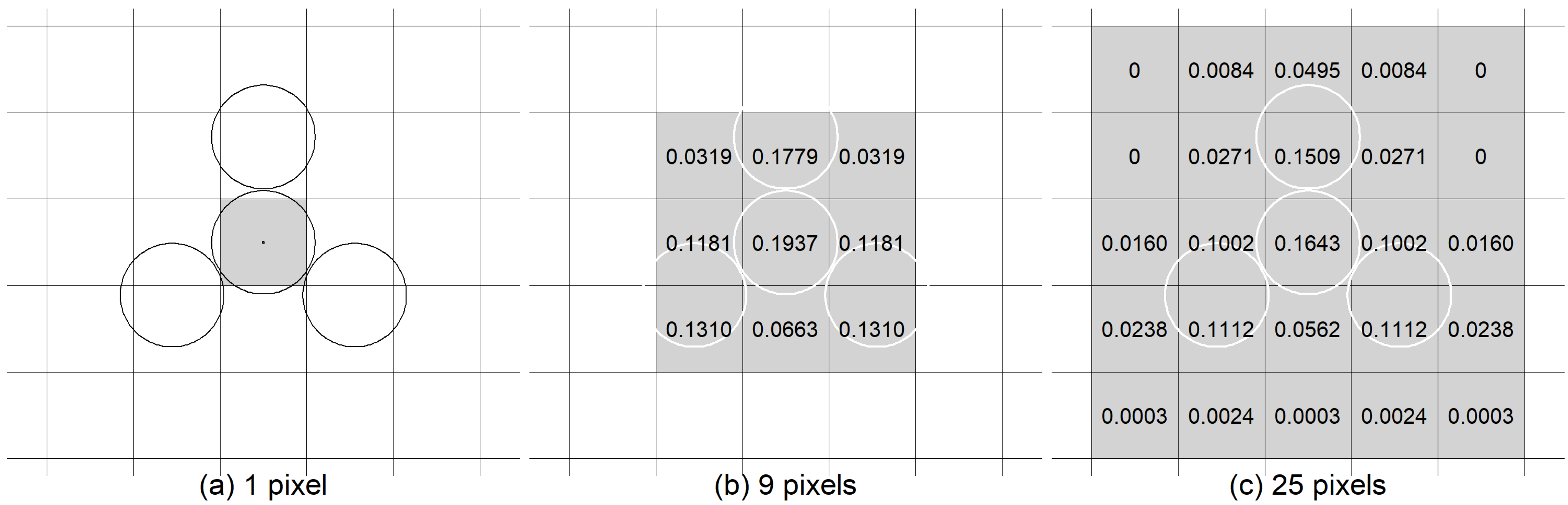
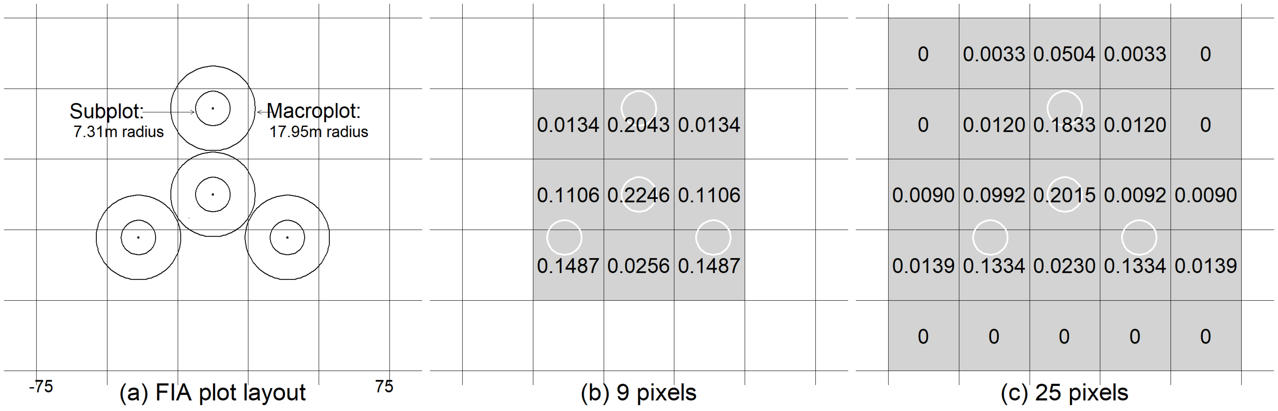
49 pixelsweights for macroplots based on pixel weight calculation (Figure 2b)
525 pixelsequal weight (1/25) applied to 25 pixels
625 pixelsweights for macroplots based on pixel weight calculation (Figure 2c)
Table 3. RdNBR—AIC, ΔAIC, RMSPE and bias for the logistic regression using RdNBR to predict the ground-based burn severity expressed as % Mort Tally. The scenario with a ΔAIC of 0 has the lowest AIC.
ScenarioDescriptionAICΔAICRMSPEBias
11 pixel4139.56252.660.1950.010
29 pixels with equal weights3906.6819.790.1880.012
39 pixels with centre pixel counted twice3893.696.800.1870.012
49 pixels with macroplots pixel weights3886.890.000.1870.012
525 pixels with equal weights4362.60475.710.2050.014
625 pixels with macroplots pixel weights3920.6033.710.1880.012
Table 4. RdNBR—Fit statistics for the ordinal regression using RdNBR as the predictor variable and 4-class ground-based burn severity where very low and low classes were combined. The scenario with a ΔAIC of 0 has the lowest AIC.
ScenarioDescriptionAICΔAICKappaWeighted Kappa% Correctly Classified
11 pixel726.2624.600.500.6965%
29 pixels with equal weights703.441.780.510.7066%
39 pixels with centre pixel counted twice701.660.000.510.7066%
49 pixels with macroplots simulation weights702.280.620.500.7065%
525 pixels with equal weights745.9344.270.460.6662%
625 pixels with macroplots simulation weights704.472.810.500.7065%
Table 5. RdNBR confusion matrix for scenario 3 where the remotely-sensed metric is calculated as the equally-weighted average of 9 pixels, and the ground-based burn severity has 4 classes.
Predicted Ground Burn SeverityActual Ground Burn Severity
Very Low\LowModerateModerately SevereSevere
Very Low\Low81.8%44.7%3.3%1.1%
Moderate17.6%41.7%32.8%6.3%
Moderately Severe0.5%10.7%36.1%12.6%
Severe0.5%2.9%27.9%80.0%
Table 6. RdNBR confusion matrix for scenario 4 where the remotely-sensed metric is calculated as the weighted average of 9 pixels based on macroplot pixel specific weights, and the ground-based burn severity has 4 classes.
Predicted Ground Burn SeverityActual Ground Burn Severity
Very Low\LowModerateModerately SevereSevere
Very Low\Low82.4%44.7%3.3%1.1%
Moderate16.6%40.8%36.1%6.3%
Moderately Severe0.5%11.7%31.1%13.7%
Severe0.5%2.9%29.5%78.9%
Table 7. Offset adjusted dNBR confusion matrix for scenario 4 where the remotely-sensed metric is calculated as the weighted average of 9 pixels based on the macroplot pixel specific weights, and the ground-based severity has 4 classes.
Predicted Ground Burn SeverityActual Ground Burn Severity
Very Low\LowModerateModerately SevereSevere
Very Low \Low82.9%46.6%9.8%5.3%
Moderate15.5%38.8%37.7%14.7%
Moderately Severe0.5%2.9%13.1%3.2%
Severe1.1%11.7%39.3%76.8%
Publisher’s Note: MDPI stays neutral with regard to jurisdictional claims in published maps and institutional affiliations.

