Article

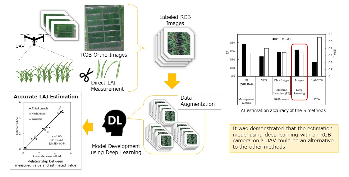
Feasibility of Combining Deep Learning and RGB Images Obtained by Unmanned Aerial Vehicle for Leaf Area Index Estimation in Rice

Graduate School of Agriculture, Tokyo University of Agriculture and Technology, Fuchu, Tokyo 183-8509, Japan
*
Author to whom correspondence should be addressed.
Remote Sens. 2021, 13(1), 84; https://doi.org/10.3390/rs13010084
Submission received: 27 October 2020 / Revised: 9 December 2020 / Accepted: 24 December 2020 / Published: 29 December 2020
(This article belongs to the Special Issue Deep Learning and Remote Sensing for Agriculture)

Abstract

:
Leaf area index (LAI) is a vital parameter for predicting rice yield. Unmanned aerial vehicle (UAV) surveillance with an RGB camera has been shown to have potential as a low-cost and efficient tool for monitoring crop growth. Simultaneously, deep learning (DL) algorithms have attracted attention as a promising tool for the task of image recognition. The principal aim of this research was to evaluate the feasibility of combining DL and RGB images obtained by a UAV for rice LAI estimation. In the present study, an LAI estimation model developed by DL with RGB images was compared to three other practical methods: a plant canopy analyzer (PCA); regression models based on color indices (CIs) obtained from an RGB camera; and vegetation indices (VIs) obtained from a multispectral camera. The results showed that the estimation accuracy of the model developed by DL with RGB images (R2 = 0.963 and RMSE = 0.334) was higher than those of the PCA (R2 = 0.934 and RMSE = 0.555) and the regression models based on CIs (R2 = 0.802-0.947 and RMSE = 0.401–1.13), and comparable to that of the regression models based on VIs (R2 = 0.917–0.976 and RMSE = 0.332–0.644). Therefore, our results demonstrated that the estimation model using DL with an RGB camera on a UAV could be an alternative to the methods using PCA and a multispectral camera for rice LAI estimation.

Graphical Abstract

1. Introduction

Leaf area index (LAI), which represents one half of the total green leaf area (i.e., half of the total area of both sides of all green leaves) per unit horizontal ground surface area [1], is a key vegetation parameter for assessing the mass balance between plants and the atmosphere [2,3], and plays an important role in crop growth estimation and yield prediction [4,5,6]. The efficiency of light capture and utilization are the ultimate factors limiting crop canopy photosynthesis, and LAI primarily determines the interception rate of solar radiation by a crop. Hence, accurate LAI estimation is an important to evaluate crop productivity. Direct LAI measurements have been performed by destructive sampling, but this approach requires a great deal of labor and time. Moreover, it is often difficult to obtain a representative value of the plot because only a part of the plot can be surveyed by direct sampling. Therefore, in recent years, various indirect methods for LAI estimation have been developed to solve these problems.
One of the widely used estimation methods is an indirect measurement using optical measuring devices. The plant canopy analyzer (PCA) is a typical optical measuring device used for this purpose. The PCA can measure LAI in a non-destructive manner by observing the transmitted light in the plant community with a special lens and measuring the rate of its attenuation [7]. It has come to be widely used as an efficient measurement method. Recently, many studies have used the PCA to obtain the ground-measured LAI as validation data for remote sensing [8,9,10].
On the other hand, indirect estimation methods using handheld or fixed-point cameras have also been studied. Mainly two types of cameras are used in these estimation methods: an RGB camera of the type used for general photography, which can acquire the brightness of red, blue, and green, and a multispectral camera that can measure the reflectance of the light in a wider variety of wavelength ranges. Several methods for estimating LAI using these cameras have been developed. Among them, a method using regression models with color indices (CIs) calculated from the digital number (DN) of light in the visible region (red, blue, and green) obtained from RGB cameras and a similar method using regression models with vegetation indices (VIs) calculated from the reflectance of light in a wider variety of wavelength ranges such as near-infrared obtained from multispectral cameras have been widely studied [11,12,13,14]. However, LAI estimation with handheld or fixed-point cameras can collect data only in a very limited area in a field. Therefore, a more effective LAI estimation method that enables data acquisition in a wider area using remote sensing by an unmanned aerial vehicle (UAV) has been proposed [15]. UAV has an remarkable advantage in that it has a very high temporal and spatial resolution compared to satellite [16]. As such, it is invaluable for screening of large number of breeding lines and monitoring within-field variability in precision agriculture. The main traditional estimation methods used in conjunction with UAVs are a method based on CIs obtained from the RGB camera and a method based on VIs obtained from the multispectral camera [11,17,18]. It is known that VIs, which contain the reflectance in the near-infrared (NIR) region, are more accurate than CIs, which contain only the visible light region [19]. However, multispectral cameras are more expensive than RGB cameras in general, and low-cost consumer UAVs equipped with RGB cameras for monitoring crop growth have recently been attracting attention [20]. Therefore, it is necessary to improve the accuracy of LAI estimation by UAVs equipped with RGB cameras.
In the last several years, an increasingly broad range of machine-learning algorithms has been used to in an attempt to improve the accuracy of LAI estimation via remote sensing technology [21,22,23,24,25]. In these studies, various types of LAI-related data (VIs, CIs, reflectance and texture index, etc.) extracted from the images were used as input data of several machine-learning algorithms to develop more accurate LAI estimation models, and their usefulness was demonstrated. However, deep learning (DL), which is the latest machine-learning algorithm, achieves much higher recognition accuracy in image recognition tasks than previous algorithms [26], and has been applied to crop growth estimation during growth duration in several reports, though its applicability to various other tasks in agricultural research, such as disease detection [27], land cover classification [28], plant recognition [29], identification of weeds [30], prediction of soil moisture content [31], and yield estimation [32], is still under investigation.
DL is a machine-learning algorithm that mimics the learning system of humans. A mathematical model called a neural network, which imitates a neurotransmission circuit of the human brain, is multiply incorporated in the algorithm. High accuracy can be achieved by building a proper network. In particular, it is known that extremely high-precision image recognition can be performed by incorporating a type of network known as a convolutional neural network (CNN) [33]. In the conventional machine-learning algorithm, the limit is that only simple numerical information can be used as input data. By applying CNN in DL, not only the simple numerical information extracted from the images but also the images themselves can be utilized as input data, potentially leading to the development of a more accurate LAI estimation model.
However, the feasibility of combining DL and RGB images obtained by UAV for LAI estimation in rice has not been adequately investigated, and the accuracy of this approach must be relativized in order to evaluate its potential applicability. Therefore, in this research, in order to refine the process of LAI estimation in rice using an RGB camera mounted on a UAV, we examined whether estimation models developed by DL with the RGB images as input data could be an alternative to existing LAI estimation methods using PCA, regression models based on indices extracted from RGB or multispectral images and estimation models developed with machine-learning algorithms.

2. Materials and Methods

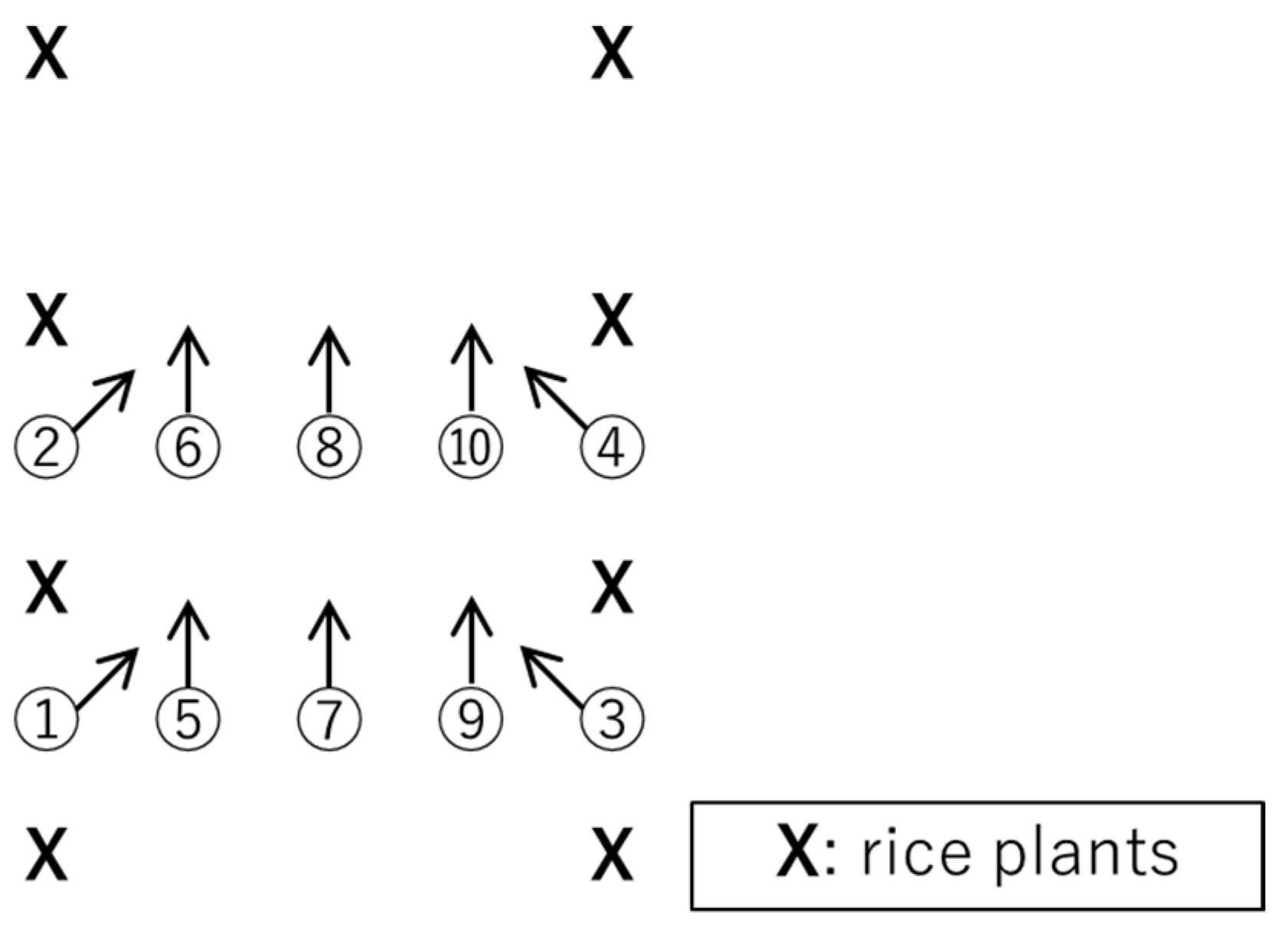
2.1. Experimental Design and Data Acquisition

The field experiment was conducted at a paddy field in the Field Museum Honmachi, Tokyo University of Agriculture and Technology, Honmachi, Fuchu-shi, Tokyo (35.41N and 139.29E) in 2019. Three rice varieties, Akitakomachi (Japonica), Koshihikari (Japonica) and Takanari (Indica) were used, and two nitrogen fertilization levels including the non-fertilized area (0N) and the fertilized area (+N: 2 g/m2 was applied as a basal on 23 May, and 2 g/m2 was applied twice as top dressing on 20 June and 17 July) were set in a split-plot design with three replications with the fertilizer treatment as the main plot. In addition, 10 g/m2 of P2O5 and K2O were applied as a basal on May 15. Transplanting was carried out on 22 May with a planting density of 22.2 hills/m2 (30 cm × 15 cm) with 3 plants per hill.
An Inspire2 (DJI) was used as the UAV, and it was equipped with a multispectral camera (RedEdge-MX; Micasense) and an RGB camera (Zenmuse X4S; DJI) with reference points set up at the four corners of the experimental field using a flight planning application (Atlas Flight, Micasense; Pix4D capture, Pix4D). The wavelength and the resolution of bands of each camera are shown in Table 1. The aerial images were taken above the rice canopy at an altitude of 30 m with both of forward and lateral overlap rate of 80% and a speed of 3 m/s. On the next day, LAI was measured at 10 points under eight hills (60 cm × 60 cm) per plot with PCA (LAI-2200; LI-COR), and the average of 10 points was used as the representative value of the plot. The detail of the measurement was shown in Figure 1. To reduce the influence of direct light and the observer, a view cap with a viewing angle of 90 degrees was attached to the sensor of the PCA, and the measurements were carried out during cloudy weather or when the sun’s altitude was low. Then, the eight hills were harvested from each plot and separated into each organ (leaves, stems, and roots), the leaf area was measured using an automatic area meter (AAM-9A; Hayashi Denko), and the ground-measured LAI of each plot was obtained by dividing by the occupied area of the eight hills (60 cm × 60 cm). The above survey was conducted every two weeks from the date of transplanting to the date of heading.

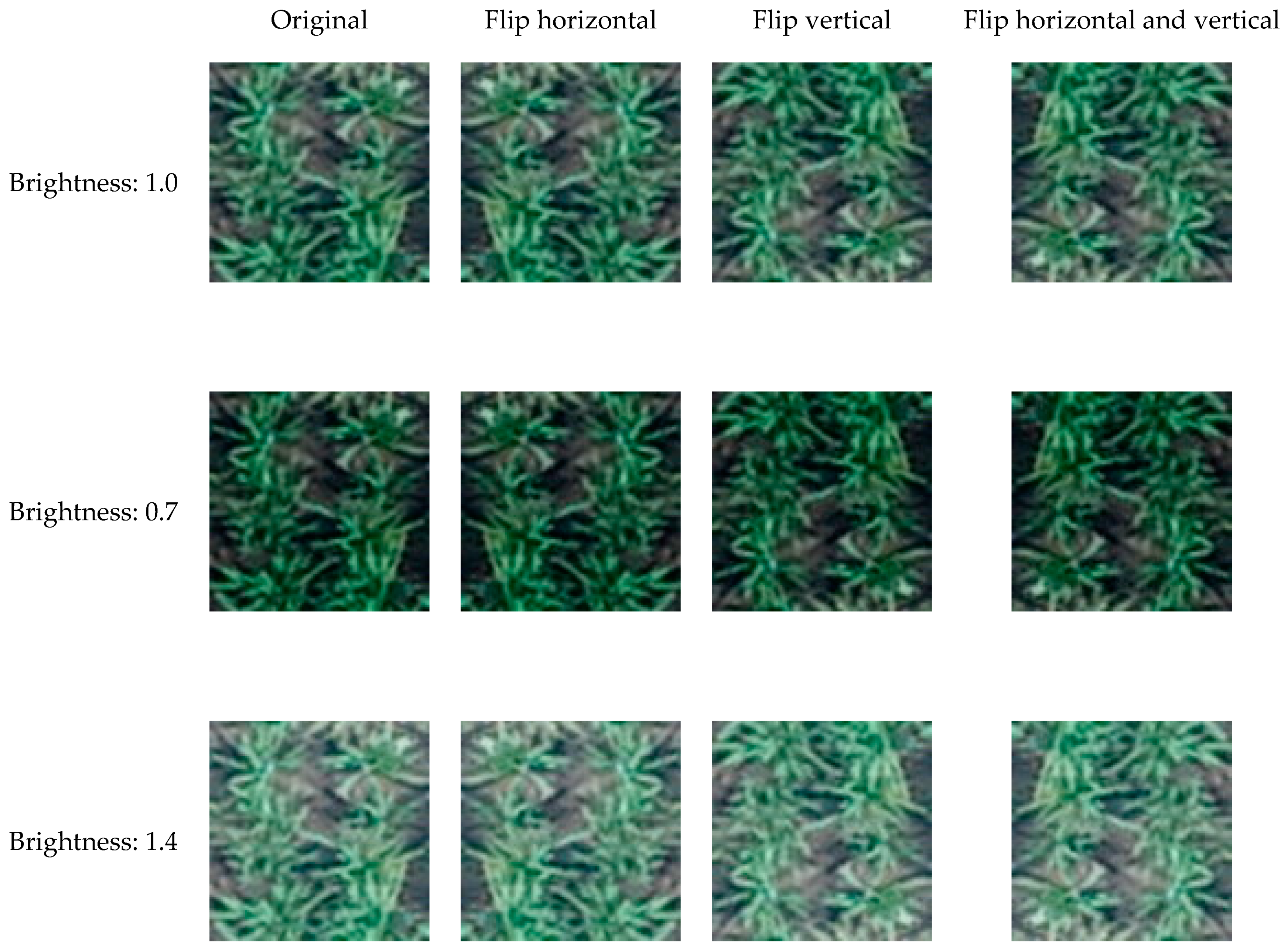
2.2. Image Processing

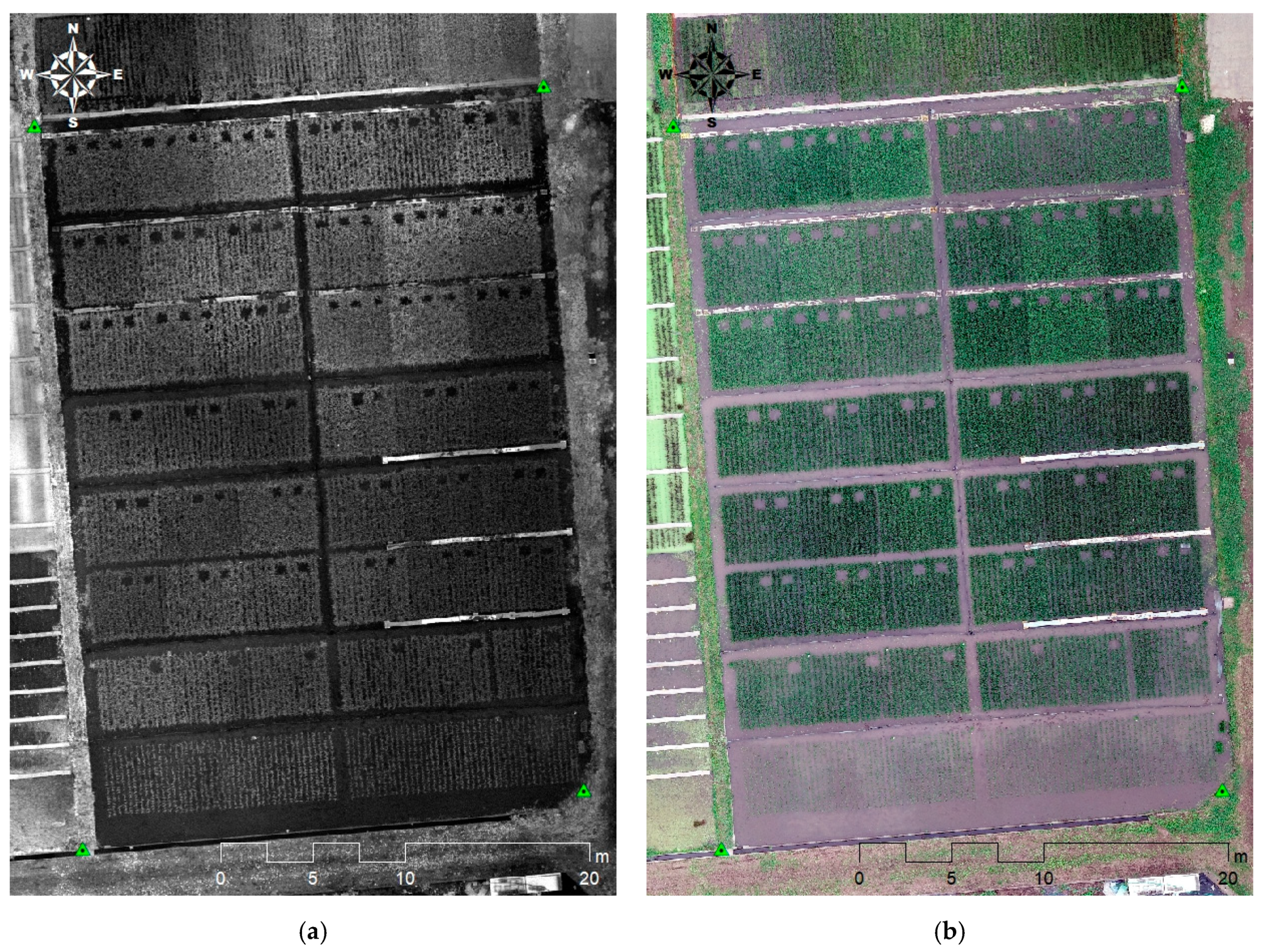
2.2.1. Generation of Ortho-Mosaic Images

The coordinates of the reference points installed at the four corners of the test field were obtained by closed traverse surveying with reference to the Japan Geodetic System 2011 Plane Cartesian Coordinate System 9 as a map projection method, and these four points were used as ground control points (GCPs) (Figure 2).
Each ortho-mosaic image was created from 5-band multispectral images and RGB images taken with the UAV. Tie points were automatically detected from the overlapping area between aerial images, and camera calibration (correction of the lens focal length, principal point position, and radial and tangential distortion) was performed with the tie points. After that, parameters of external orientation (camera position and tilting angle) were estimated using the detected tie points and the four installed GCPs, and the 3D model was developed. This processing was performed so that the accuracy of GCPs was within 1 pixel. Ortho-mosaic images (orthophoto images) of 5-band multispectral cameras and RGB cameras were generated from each of the 3D models (Figure 2). The resolutions of these images were 12 mm and 9 mm, respectively. When generating the multispectral ortho-mosaic images, the attached light-intensive sensor automatically converts DN into the reflectance of each band and the reflectance was used for calculation of VIs. As for RGB ortho-mosaic images, DNs were used for calculation of CIs. Metashape (Agisoft) was used for the above processing.

2.2.2. Calculation of Vegetation Indices and Color Indices

The average reflectance of the eight hills (60 cm × 60 cm) in each plot, which is taken for destructive LAI measurements, was extracted from the multispectral ortho-mosaic images of each band (blue, green, red, rededge and near-infrared) using polygons (15 cm × 30 cm) including each hill using a geographical information system (ArcMap, Esri) (Figure 3).
Various VIs for which the relationship with LAI have been reported were calculated from the multispectral reflectance. In this study, four types of VIs, normalized difference vegetation index (NDVI), simple ratio (SR), modified simple ratio (MSR), and soil adjusted vegetation index (SAVI), were calculated with the two bands of reflectance (λ1, λ2) (Table 2). In general, these VIs are often used with substitution of the reflectance of near-infrared and red for λ1 and λ2, respectively, but in our present experiments, in addition to these substitutions, we also substituted the reflectance of near-infrared and rededge, and the reflectance of rededge and red for λ1 and λ2, respectively. In total, 12 VIs were calculated from the reflectance obtained from the multispectral ortho-mosaic images in this study (Table 2).
For the RGB ortho-mosaic images containing the DNs of three colors (red, green, and blue), small images containing eight hills (60 cm × 60 cm) were cut out at a resolution of 100 × 100 pixels (these cut-out RGB images were also used as input data for DL) (Figure 4) and the DNs of three colors (red (R), green (G), and blue (B)) were acquired using an image processing software package (ImageJ; Wayne Rasband). The normalized DNs of the three colors, r, g, and b, are calculated by dividing the original DNs of red (R), green (G), and blue (B) by the sum of these three original DNs as follows:
r = R/(R + G + B),
g = G/(R + G + B),
b = B/(R + G + B).
In this study, nine types of CIs, visible atmospherically resistant index (VARI), excess green vegetation index (E × G), excess red vegetation index (E × R), excess blue vegetation index (E × B), normalized green-red difference index (NGRDI), modified green red vegetation index (MGRVI), green leaf algorithm (GLA), red green blue vegetation index (RGBVI), and vegetativen (VEG), whose relationship with LAI have been reported were calculated from the normalized DNs (Equations (1)–(3)) obtained from the RGB camera (Table 2).

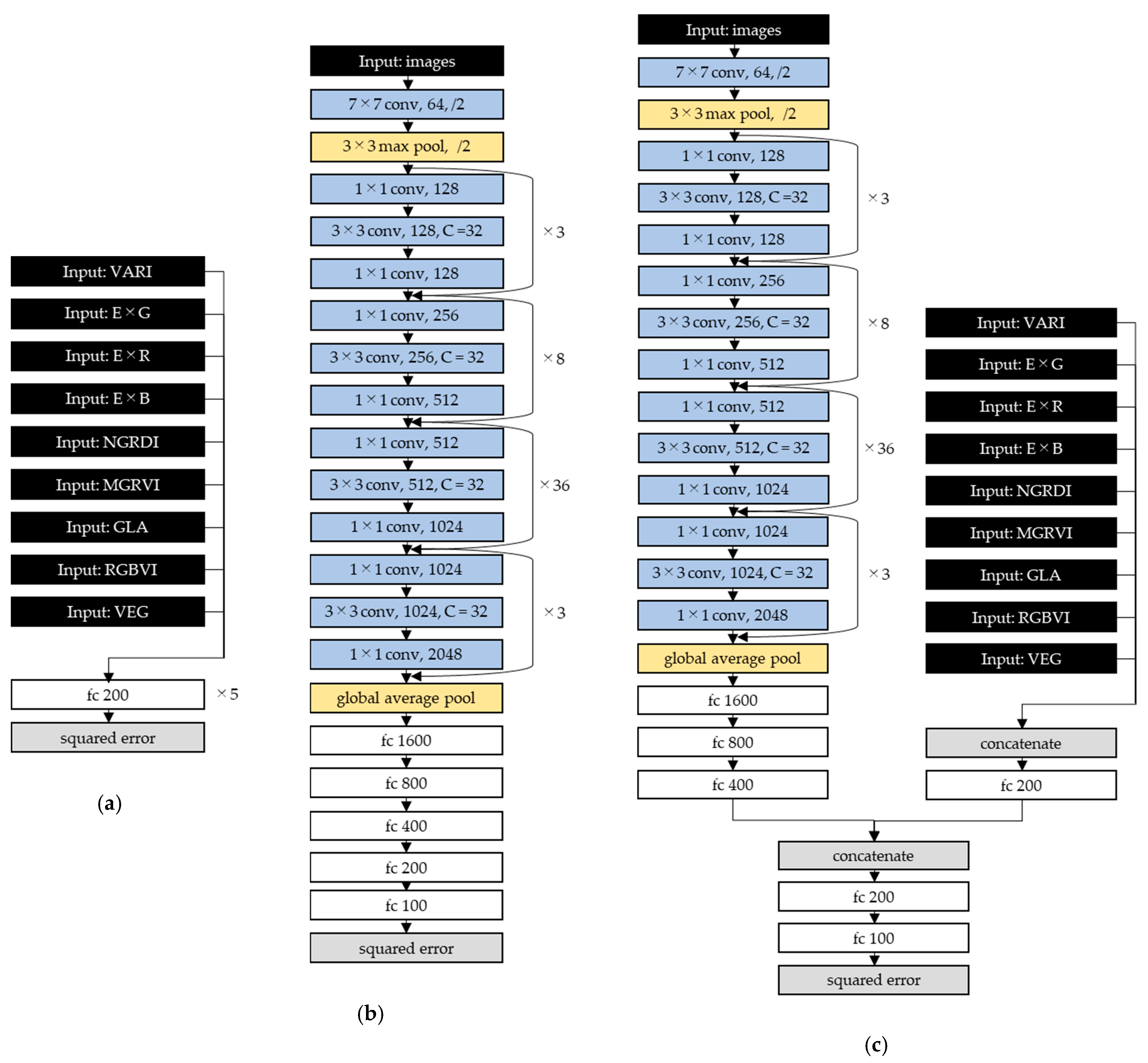
2.3. Estimation Model Development and Accuracy Assessment

Replication 1 and 2 were used as training data for model construction (n = 48), and replication 3 was used as validation data to verify the model accuracy (n = 24). The RGB images for the training data of DL were inflated 12 times (n = 576) by flipping left and right and upside down and changing the brightness (0.7, 1.4 times) (Figure 5).
Based on each of the calculated VIs and CIs, regression models of the ground-measured LAI were developed by the least-square method, and their accuracy was verified.
In a previous study, CIs were applied for the machine-learning algorithm to develop LAI estimation models [22]. Therefore, in this research, CIs were also used as input data for machine-learning-algorithms and DL in addition to RGB images for relative evaluation. In total, three patterns of input datasets (nine types of CIs, RGB images, and nine types of CIs and RGB images) were prepared for machine-learning algorithms and DL to assess the potential estimation accuracy of the RGB camera. After that, the LAI estimation models by machine-learning algorithms and DL using each of the input datasets were constructed, then their accuracy was assessed.
As a comparative analysis method for DL, four kinds of machine-learning algorithms, artificial neural network (ANN), partial least squares regression (PLSR), random forest (RF) and support vector regression (SVR), other than DL were used in this study. Scikit-learn, an open source library of Python was used for model development. Main tuning parameters of each machine-learning algorithms, ANN: the number of hidden layer neurons and max iterations, PLSR: the number of explanatory variables, RF: the number of tree (ntree) and the number of features to consider (mtry), SVR: gamma, C and epsilon, were adjusted using a grid search before development of the estimation models.
The Neural Network Console (SONY), which is an integrated development tool for the DL program, was used for development of the estimation model. When developing an estimation model using the nine types of CI data, we designed a simple neural network with 5 fully connected layers (Figure 6). The CNN, which enables area-based feature extraction and robust recognition against image movement and deformation, is known to be an effective layer for the task of image recognition [33]. Deepening the CNN layers plays an important role for accurate image recognition, because each layer extracts more sophisticated and complex features from images. ResNet is a network structure that has been successfully used to layer CNNs up to 152 layers, and it achieved much higher accuracy than conventional network structures and higher accuracy than humans for this purpose [45]. However, ResNet has a disadvantage in its complexity of architecture. ResNeXt achieved better accuracy than ResNet and succeeded in reducing the calculation cost by introducing the technique of grouped convolution to ResNet [46]. Moreover, ResNeXt showed its high potential in agricultural researches [47,48]. In this research, ResNeXt was modified so that our datasets were applicable and used to develop LAI estimation models from input datasets containing images (RGB images, and nine types of CIs and RGB images) (Figure 6). Hyper parameters were determined as shown in Table 3.

3. Results

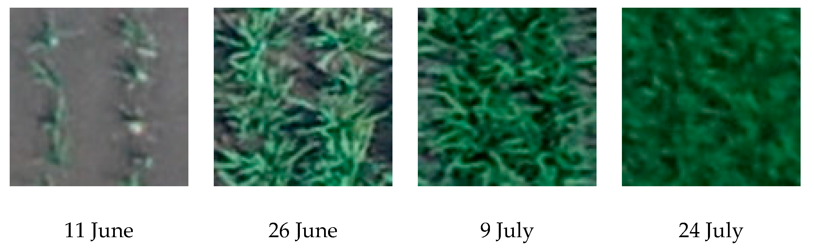
3.1. Variations of the Ground-Measured Leaf Area Index

Figure 7 shows seasonal variations of the ground-measured LAI under each condition (three rice varieties and two nitrogen management levels) observed in this study. LAI gradually increases from the transplanting (Figure 7) and ranged from 0.135 to 6.71 during growth duration. Significant differences in fertilizer management from the 1st to 3rd sampling and varieties at the first sampling were observed.

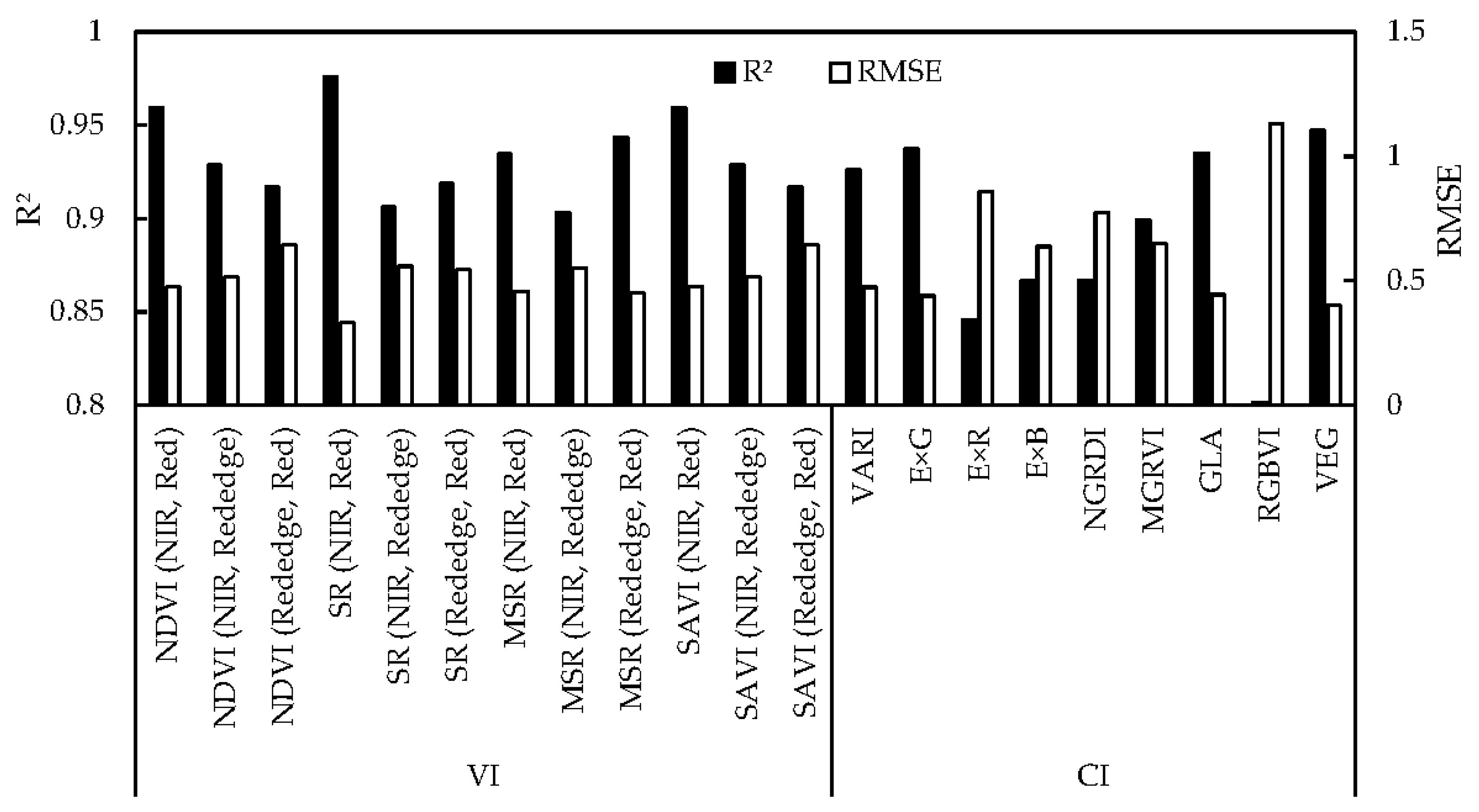
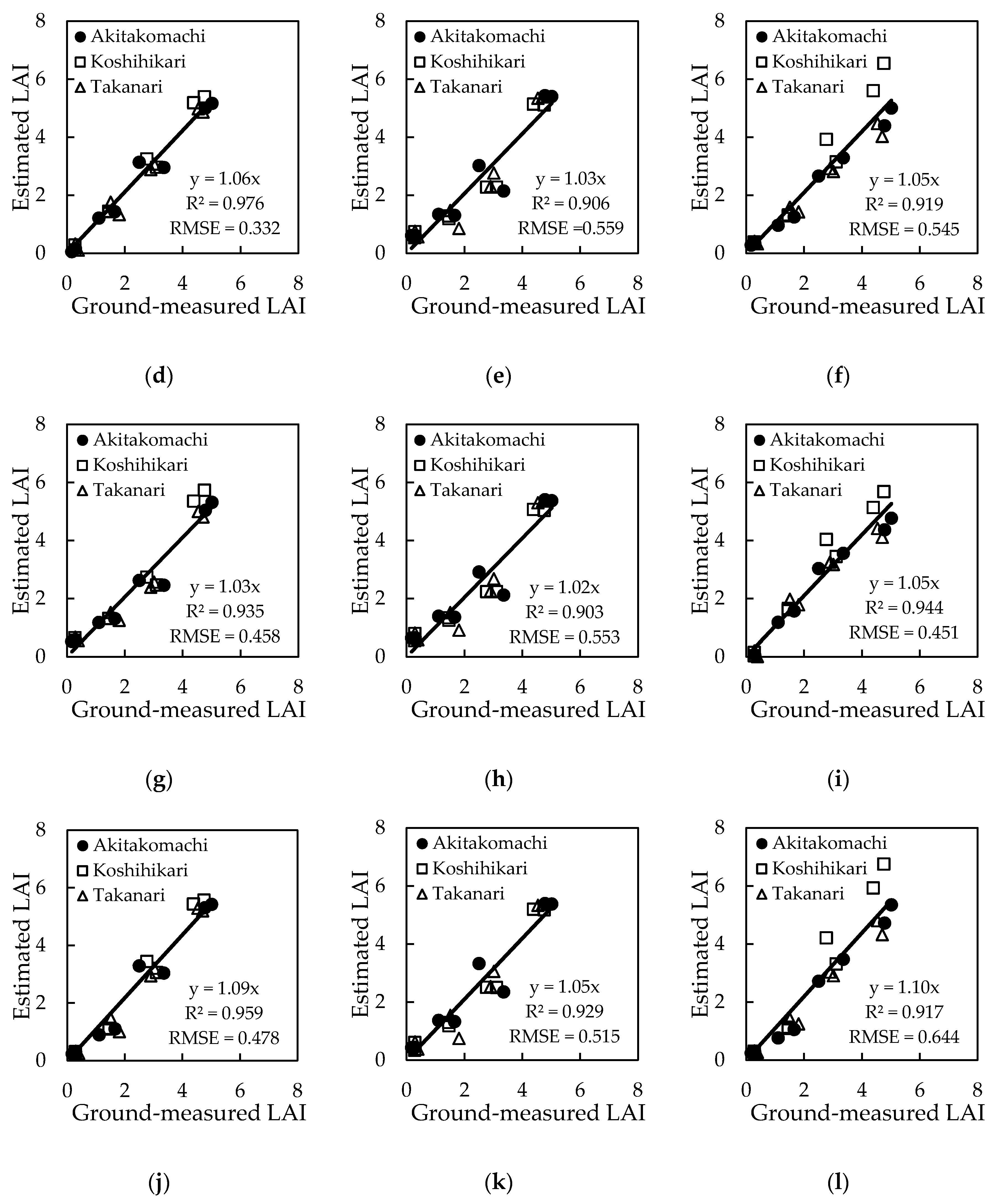
3.2. Regression Models Using Each of VIs and CIs

Regression equations of the LAI estimation models based on each index are shown in Table 4. A comparison of the estimation accuracy of each model is shown in Figure 8. Correlations between the ground-measured LAI and estimated LAI of the regression models based on each of the VIs and CIs are shown in Figure 9 and Figure 10, respectively. The estimation accuracy of the LAI of the regression models differed depending on the indices, and the coefficient of determination ranged from 0.802 to 0.976 and root mean squared error (RMSE) ranged from 0.332 to 1.13 (Figure 8, Figure 9 and Figure 10). In the estimation models based on VIs, the coefficient of determination ranged from 0.906 to 0.976 and RMSE ranged from 0.332 to 0.644 (Figure 8 and Figure 9). In the estimation models based on CIs, the coefficient of determination ranged from 0.802 to 0.947 and RMSE ranged from 0.401 to 1.13 (Figure 8 and Figure 10). Generally, the estimation model based on VIs acquired from the multispectral camera exhibited higher accuracy than the model based on CIs acquired from the RGB camera (Figure 8). SR (NIR, Red) achieved the highest accuracy of all indices (R2 = 0.976 and RMSE = 0.332) followed by NDVI (NIR, Red) (R2 = 0.959 and RMSE = 0.475) and SAVI (NIR, Red) (R2 = 0.959 and RMSE = 0.478) (Figure 8 and Figure 9a,d,j). VEG showed the highest accuracy of all CIs (R2 = 0.947 and RMSE = 0.401) followed by E × G (R2 = 0.937 and RMSE = 0.440) and GLA (R2 = 0.935 and RMSE = 0.444) (Figure 8 and Figure 10b,g,i).

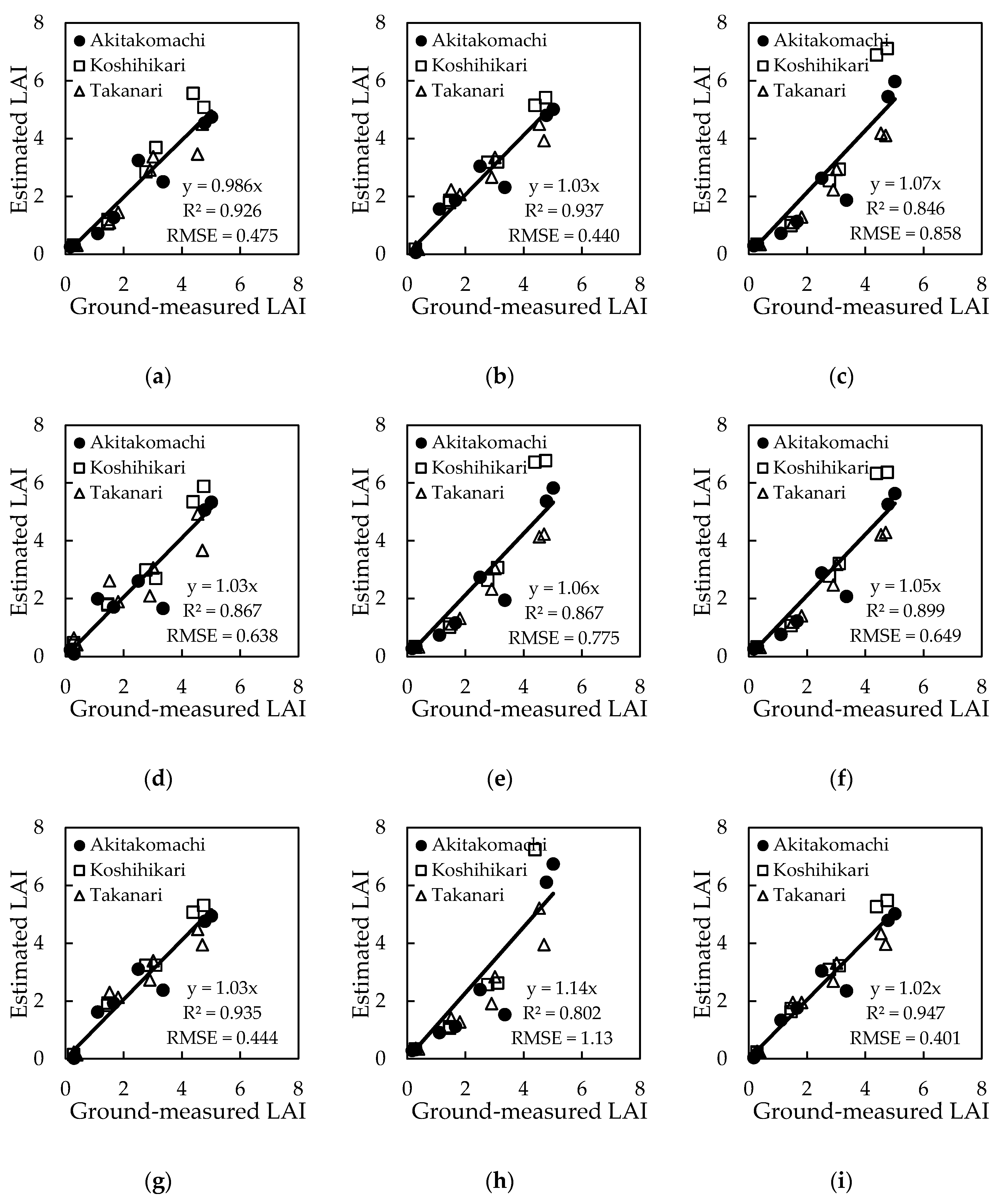
3.3. Estimation Models by Machine-Learning Algorithms Other Than Deep Learning

Table 5 shows the accuracy of the LAI estimation model developed by four kinds of machine-learning algorithms using three patterns of input datasets, nine types of CIs, RGB images, and nine types of CIs and RGB images obtained from the RGB camera. As for ANN, PLSR and SVR, the highest accuracy was achieved when the input data was CIs (R2 = 0.940 and RMSE = 0.401, R2 = 0.939 and RMSE = 0.422 and R2 = 0.945 and RMSE = 0.399, respectively). RF achieved the highest accuracy when the input data was nine types of CIs and RGB images, which was the highest accuracy in all combinations (R2 = 0.957 and RMSE = 0.342).

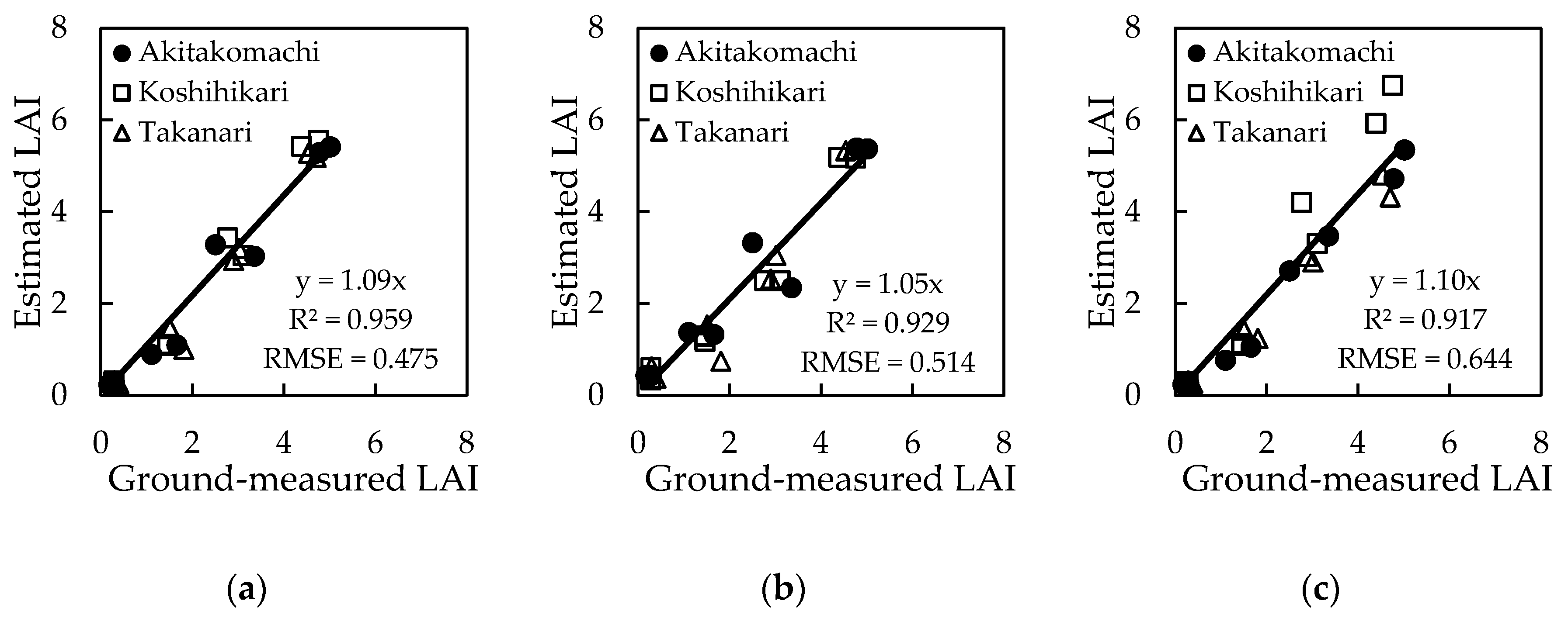
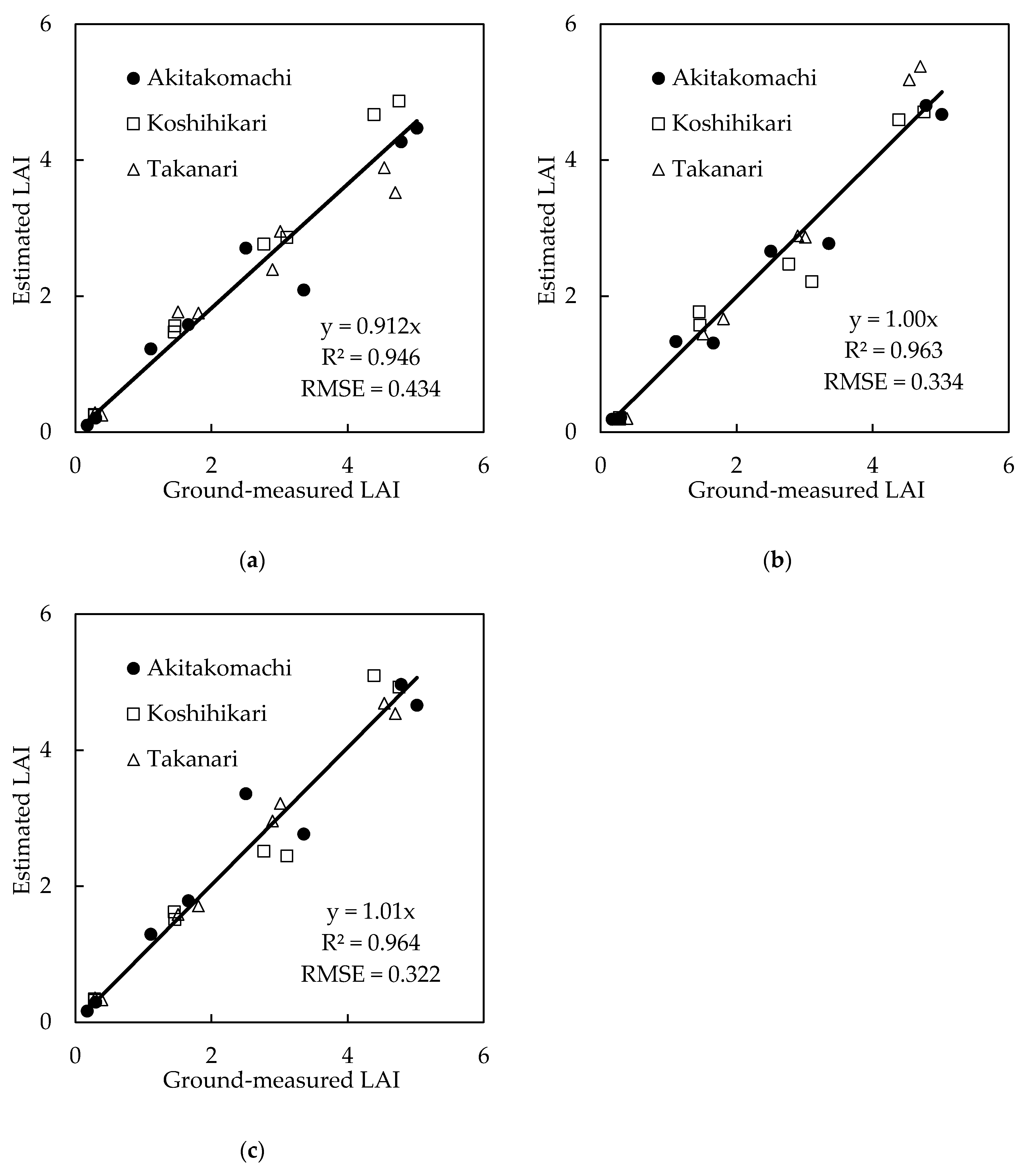
3.4. Estimation Models by Deep Learning

Table 6 and Figure 11 shows the accuracy of training and validation data with the LAI estimation model constructed by DL using three patterns of input datasets: nine types of CIs, RGB images, and nine types of CIs and RGB images obtained from the RGB camera, respectively. Training data was fitted with R2 = 0.900 and RMSE = 0.605 for CIs, R2 = 0.979 and RMSE = 0.280 for images and R2 = 0.989 and RMSE = 0.203 for CIs + images, respectively (Table 6). The coefficient of determination ranged from 0.946 to 0.964, and RMSE ranged from 0.322 to 0.434. The estimation model using nine types of CIs as input data underestimated the ground-measured LAI; the estimation accuracy of this model was lower than those of the other two estimation models and there was no improvement from the regression model of VEG, which achieved the highest accuracy in all CIs (R2 = 0.946 and RMSE = 0.434) (Figure 11a). Higher accuracy was achieved in the estimation model using RGB images as input data (R2 = 0.963 and RMSE = 0.334) (Figure 11b), and little improvement was observed in the estimation model using nine types of CIs and RGB images as input data, with values of R2 = 0.964 and RMSE = 0.322 (Figure 11c). These two models containing RGB images as input data achieved almost the same accuracy as the regression model of SR (NIR, Red), which achieved the highest accuracy in VIs (Figure 9d).

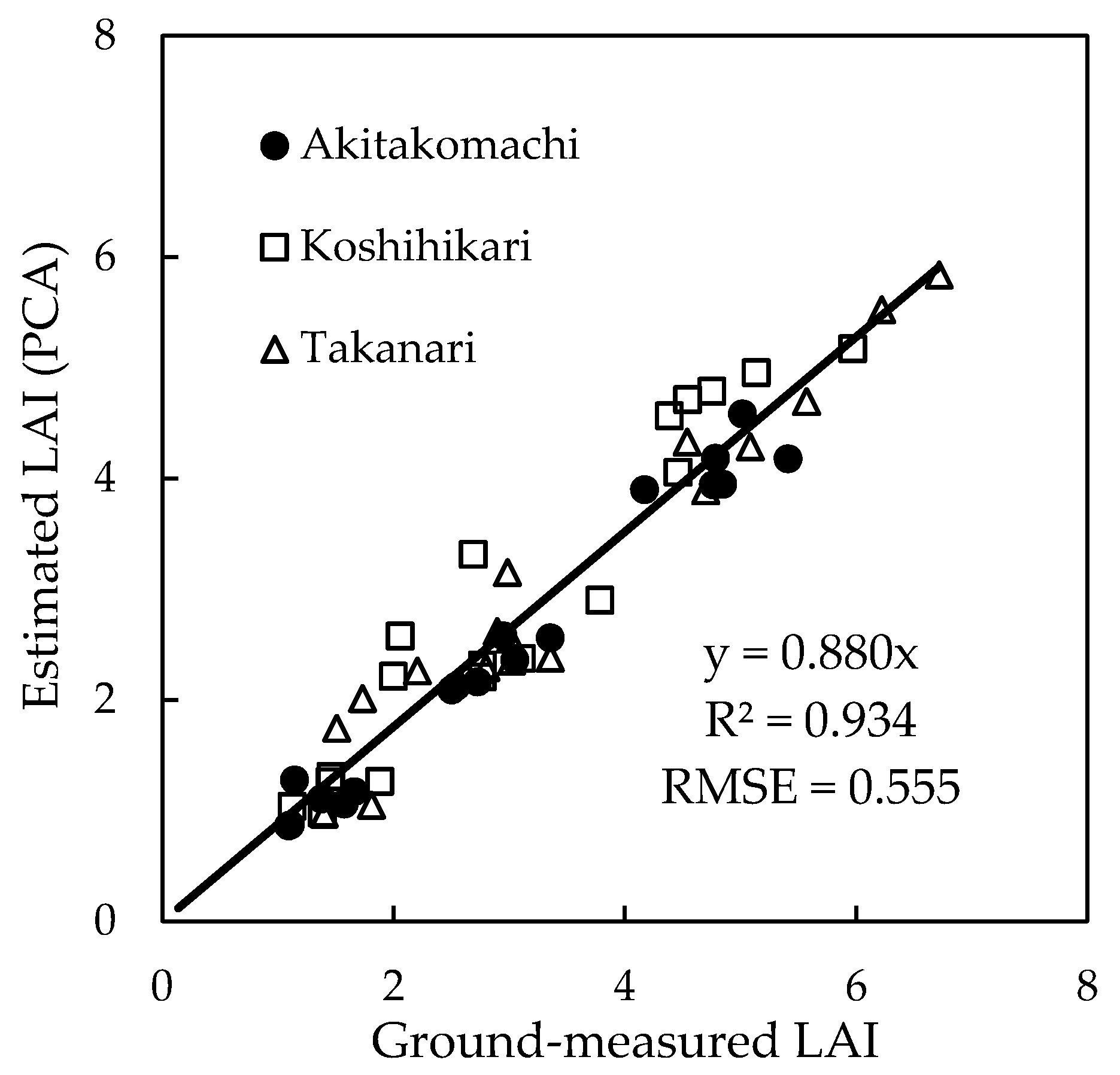
3.5. Plant Canopy Analyzer
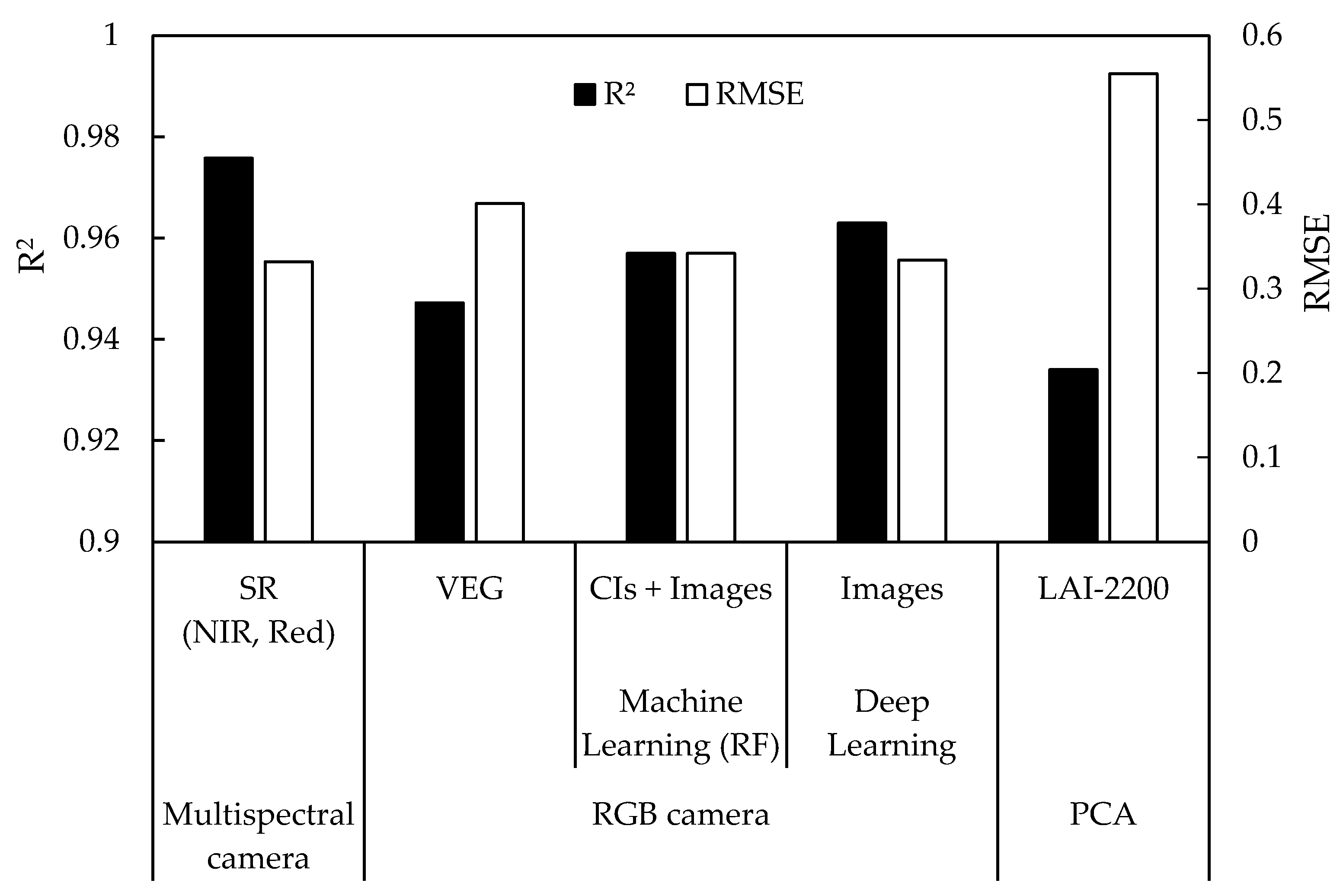
Figure 12 shows the relationship between the measured LAI values and the measured values by PCA under each of the variety and fertilization conditions. The measured values with PCA could explain the measured LAI with an accuracy of R2 = 0.934 and RMSE = 0.308 without significant difference in variety and fertilization level (Figure 12). However, PCA underestimated the ground-measured LAI by 12% (Figure 12).

4. Discussion

In this study, we attempted to improve the accuracy of LAI estimation in rice using an RGB camera mounted on a UAV by developing an estimation model using DL with the images as input data, and then compared the estimation accuracies of the resulting model and other hands-on approaches. The model using DL with RGB images could explain the large variation of LAI of different rice varieties grown under different fertilizer conditions with high accuracy. The range of LAI in the present study (from 0.135 to 6.71) was sufficiently large to cover the variations of rice leaf area grown under irrigated fields of various environments [49]. Our results thus demonstrated that the model using DL with RGB images could provide an alternative to the methods using a multispectral camera and PCA for the estimation of rice LAI. Figure 13 summarizes the LAI estimation accuracy of five methods: regression models based on SR (NIR, Red) and VEG, which showed the highest accuracy among all indices and all CIs, respectively; estimation models developed by RF using nine types of CIs and RGB images, which showed the highest accuracy in all machine-learning algorithms; estimation models developed by DL using RGB images; PCA (LAI-2200). We will discuss these results in detail.
First, we examined the accuracy of LAI estimation by the regression models based on each index. Since spectral information is affected by various factors, including plant morphology, soil background, and the shooting environment [14,50,51], the optimal index for LAI estimation depends on prior information [52,53,54]. Under the condition in this experiment, SR (NIR, Red) was the most favorable of the indices (R2 = 0.976 and RMSE = 0.332), and VEG was the most accurate of the CIs (R2 = 0.947 and RMSE = 0.401) (Table 4, Figure 8 and Figure 13). Although the estimation accuracy varied depending on the index, the VIs obtained from the multispectral camera generally performed better than the CIs obtained from the RGB camera (Table 4, Figure 8), which agreed with the results of Gupta et al. [19]. The reflectance of near-infrared light is more responsive to an increase in leaf area than the reflectance of visible light, because the former is more easily affected by changes in the vegetation structure [37]. Therefore, it is considered that the VIs including the reflectance of near-infrared light acquired from a multispectral camera showed relatively high estimation accuracy.
Then, we assessed the estimation accuracy of four kinds of machine-learning algorithms using three patterns of input datasets, nine types of CIs, RGB images, and nine types of CIs and RGB images. Compared to VEG, which showed the highest estimation accuracy among the CIs acquired from the RGB camera (R2 = 0.947 and RMSE = 0.401), the estimation model developed by RF using nine types of CIs and images as input data showed an improvement (R2 = 0.957 and RMSE = 0.342) (Figure 10 and Figure 13, Table 5). Several existing researches have indicated that RF is an ideal algorithm to improve the estimation accuracy of LAI [21,22,25], and the results of this study was consistent with these reports.
Next, we tried to improve the accuracy of LAI estimation using an RGB camera on a UAV by means of a DL technique. Compared to RF, further improvement was observed in the estimation model by DL using RGB images (R2 = 0.963 and RMSE = 0.334), and its accuracy was comparable to that of SR (NIR, Red) (R2 = 0.976 and RMSE = 0.332), which showed the highest estimation accuracy among the VIs acquired from the multispectral camera (Figure 9d, Figure 11b and Figure 13). The results suggested that although the RGB camera is inferior when using only CIs, it can be made to achieve high performance equivalent to that of the multispectral camera simply by constructing an estimation model by DL with the images incorporated as input data. In the conventional machine-learning algorithms, the features must be specified in advance. In contrast, DL has the major advantage of being able to identify the characteristics of the images automatically [55]. In this research, since the training data in DL included images with a resolution of 100 × 100 pixels, which contained much more information than the CIs, the characteristics of plant morphology were recognized in greater detail. These factors were considered to be the reason for the achievement of a high estimation accuracy by DL with images.
Additionally, DL is known to be a promising algorithm to develop a robust model which could be applicable to the various conditions [56]. Therefore, there would still be room for improvement in terms of the robustness under various agricultural conditions, since the cultivars and management used in this study are limited. As training data for DL, the number of RGB images were enhanced by 12 times using flipping and changing brightness. Increasing the number of images with more diverse methods would be able to also contribute to further improvement in estimation accuracy. In addition, it is necessary to consider how much the resolution can be reduced while maintaining the explanatory accuracy of the model although we performed DL using 9 mm/pixels images in this study. Lastly, we can expect a further improvement by using multispectral images in addition to RGB images since the estimation accuracy was made better by applying RGB images to DL than the conventional method. By combining these findings with, for example, fixed-wing UAVs and high-resolution satellite sensors, this model could be applied to a wider area.
Finally, we examined the estimation accuracy of PCA, which has been widely used to obtain ground-truth data of LAI in the field of remote sensing. Although the measured value with PCA could explain the ground-measured LAI with an accuracy of R2 = 0.934 and RMSE = 0.555, this was lower than the accuracies by a multispectral camera (the regression model based on SR (NIR, Red): R2 = 0.976 and RMSE = 0.332) and an RGB camera (the estimation model developed by DL using RGB images: R2 = 0.963 and RMSE = 0.334) (Figure 9d, Figure 11b, Figure 12 and Figure 13). This is because plants other than the sampled eight hills got into the view of the PCA sensor, even though a view cap was installed. In addition, PCA led to 12% underestimation of the ground-measured values (Figure 12). This result was consistent with the previous studies by Maruyama et al. [57] and Fang et al. [58], which reported that PCA underestimates the LAI measurements of rice canopy throughout the growth stage. LAI estimation with PCA is based on the assumption that the leaves are randomly distributed in space. For this reason, two factors have been reported to affect PCA-based measurement of LAI: the first is clamping, which means that parts of a plant are concentrated in one place, thereby undermining the random distribution and causing underestimation of LAI; and the second is the entry of plant components other than leaves into the field of the sensor, which causes LAI overestimation [59]. Especially in the case of rice canopies, leaf overlap [57] and the presence of stems, which were originally spatially aggregated [58], have been reported as the factors leading to clamping, and these factors are considered to be the main cause of the underestimation in this study. This underestimation could be mitigated by using four-ring data instead of five-ring data of PCA [58]. In any case, PCA can measure the canopy LAI non-destructively and rapidly, and will certainly be a useful ground-truth acquisition tool. In order to use the PCA effectively, sufficient attention should be paid to the correspondence of PCA with measured values.

5. Conclusions

In the present research, we examined whether models developed by DL using RGB images as input data could be an alternative to existing approaches for the estimation of LAI in rice using a UAV equipped with an RGB camera. Our results demonstrated that the model using DL with RGB images could estimate rice LAI as accurately as regression models based on VIs obtained from the multispectral camera and more accurately than PCA. However, the model was developed in limited cultivation conditions, varieties and area. DL has the potential to adapt to various circumstances using big data. Therefore, it would be possible to build a more robust model for wider area by accumulating data under more diverse agricultural and shooting conditions in the future.

Author Contributions

Experimental design and field data collection, T.Y., Y.I. and K.K.; Image processing, Y.T. and M.Y.; Data extraction, Y.I.; Model development, summarization of results and writing-original draft, T.Y.; Supervision, M.Y. and K.K.; Project administration and funding acquisition, K.K. All authors have read and agreed to the published version of the manuscript.

Funding

This research was funded by Science and Technology Research Partnership for Sustainable Development (SATREPS), Japan Science and Technology Agency (JST)/Japan International Cooperation Agency (JICA) (Grant No. JPMJSA1907), and Japan Society for the Promotion of Science KAKENHI (Grant No. JP20H02968 and JP18H02295).

Acknowledgments

The authors would like to acknowledge Koji Matsukawa, a technical staff member of the Field Museum Honmachi of Tokyo University of Agriculture and Technology, for his management of the paddy field.

Conflicts of Interest

The authors declare no conflict of interest.

References

  1. Lahoz, W. Systematic Observation Requirements for Satellite-based Products for Climate, 2011 Update, Supplemental Details to the Satellite-Based Component of the Implementation Plan for the Global Observing System for Climate in Support of the UNFCCC (2010 Update); World Meteorological Organization (WMO): Geneva, Switzerland, 2011; p. 83. [Google Scholar]
  2. Asner, G.P.; Scurlock, J.M.O.; Hicke, J.A. Global synthesis of leaf area index observations. Glob. Chang. Biol. 2008, 14, 237–243. [Google Scholar] [CrossRef] [Green Version]
  3. Stark, S.C.; Leitold, V.; Wu, J.L.; Hunter, M.O.; de Castilho, C.V.; Costa, F.R.C.; Mcmahon, S.M.; Parker, G.G.; Shimabukuro, M.T.; Lefsky, M.A.; et al. Amazon forest carbon dynamics predicted by profiles of canopy leaf area and light environment. Ecol. Lett. 2012, 15, 1406–1414. [Google Scholar] [CrossRef] [PubMed] [Green Version]
  4. Duchemin, B.; Maisongrande, P.; Boulet, G.; Benhadj, I. A simple algorithm for yield estimates: Evaluation for semi-arid irrigated winter wheat monitored with green leaf area index. Environ. Model. Softw. 2008, 23, 876–892. [Google Scholar] [CrossRef] [Green Version]
  5. Fang, H.; Liang, S.; Hoogenboom, G. Integration of MODIS LAI and vegetation index products with the CSM-CERES-Maize model for corn yield estimation. Int. J. Remote Sens. 2011, 32, 1039–1065. [Google Scholar] [CrossRef]
  6. Brisson, N.; Gary, C.; Justes, E.; Roche, R.; Mary, B.; Ripoche, D.; Zimmer, D.; Sierra, J.; Bertuzzi, P.; Burger, P.; et al. An overview of the crop model STICS. Eur. J. Agron. 2003, 18, 309–332. [Google Scholar] [CrossRef]
  7. Stenberg, P.; Linder, S.; Smolander, H.; Flower-Ellis, J. Performance of the LAI-2000 plant canopy analyzer in estimating leaf area index of some Scots pine stands. Tree Physiol. 1994, 14, 981–995. [Google Scholar] [CrossRef] [PubMed]
  8. Wang, C.; Nie, S.; Xi, X.; Luo, S.; Sun, X. Estimating the biomass of maize with hyperspectral and LiDAR data. Remote Sens. 2016, 9, 11. [Google Scholar] [CrossRef] [Green Version]
  9. Luo, S.; Wang, C.; Xi, X.; Nie, S.; Fan, X.; Chen, H.; Yang, X.; Peng, D.; Lin, Y.; Zhou, G. Combining hyperspectral imagery and LiDAR pseudo-waveform for predicting crop LAI, canopy height and above-ground biomass. Ecol. Indic. 2019, 102, 801–812. [Google Scholar] [CrossRef]
  10. Hashimoto, N.; Saito, Y.; Maki, M.; Homma, K. Simulation of reflectance and vegetation indices for unmanned aerial vehicle (UAV) monitoring of paddy fields. Remote Sens. 2019, 11, 2119. [Google Scholar] [CrossRef] [Green Version]
  11. Sakamoto, T.; Shibayama, M.; Kimura, A.; Takada, E. Assessment of digital camera-derived vegetation indices in quantitative monitoring of seasonal rice growth. ISPRS J. Photogramm. Remote Sens. 2011, 66, 872–882. [Google Scholar] [CrossRef]
  12. Fan, X.; Kawamura, K.; Guo, W.; Xuan, T.D.; Lim, J.; Yuba, N.; Kurokawa, Y.; Obitsu, T.; Lv, R.; Tsumiyama, Y.; et al. A simple visible and near-infrared (V-NIR) camera system for monitoring the leaf area index and growth stage of Italian ryegrass. Comput. Electron. Agric. 2018, 144, 314–323. [Google Scholar] [CrossRef]
  13. Lee, K.J.; Lee, B.W. Estimation of rice growth and nitrogen nutrition status using color digital camera image analysis. Eur. J. Agron. 2013, 48, 57–65. [Google Scholar] [CrossRef]
  14. Tanaka, Y.; Katsura, K.; Yamashita, Y. Verification of image processing methods using digital cameras for rice growth diagnosis. J. Japan Soc. Photogramm. Remote Sens. 2020, 59, 248–258. [Google Scholar]
  15. Maes, W.H.; Steppe, K. Perspectives for Remote Sensing with Unmanned Aerial Vehicles in Precision Agriculture. Trends Plant Sci. 2019, 24, 152–164. [Google Scholar] [CrossRef] [PubMed]
  16. Zhang, C.; Kovacs, J.M. The application of small unmanned aerial systems for precision agriculture: A review. Precis. Agric. 2012, 13, 693–712. [Google Scholar] [CrossRef]
  17. Kross, A.; McNairn, H.; Lapen, D.; Sunohara, M.; Champagne, C. Assessment of RapidEye vegetation indices for estimation of leaf area index and biomass in corn and soybean crops. Int. J. Appl. Earth Obs. Geoinf. 2015, 34, 235–248. [Google Scholar] [CrossRef] [Green Version]
  18. Liu, K.; Zhou, Q.B.; Wu, W.B.; Xia, T.; Tang, H.J. Estimating the crop leaf area index using hyperspectral remote sensing. J. Integr. Agric. 2016, 15, 475–491. [Google Scholar] [CrossRef] [Green Version]
  19. Gupta, R.K.; Vijayan, D.; Prasad, T.S. The relationship of hyper-spectral vegetation indices with leaf area index (LAI) over the growth cycle of wheat and chickpea at 3 nm spectral resolution. Adv. Sp. Res. 2006. [Google Scholar] [CrossRef]
  20. Lu, N.; Zhou, J.; Han, Z.; Li, D.; Cao, Q.; Yao, X.; Tian, Y.; Zhu, Y.; Cao, W.; Cheng, T. Improved estimation of aboveground biomass in wheat from RGB imagery and point cloud data acquired with a low-cost unmanned aerial vehicle system. Plant Methods 2019, 15, 1–16. [Google Scholar] [CrossRef] [Green Version]
  21. Houborg, R.; McCabe, M.F. A hybrid training approach for leaf area index estimation via Cubist and random forests machine-learning. ISPRS J. Photogramm. Remote Sens. 2018, 135, 173–188. [Google Scholar] [CrossRef]
  22. Li, S.; Yuan, F.; Ata-UI-Karim, S.T.; Zheng, H.; Cheng, T.; Liu, X.; Tian, Y.; Zhu, Y.; Cao, W.; Cao, Q. Combining color indices and textures of UAV-based digital imagery for rice LAI estimation. Remote Sens. 2019, 11, 63. [Google Scholar] [CrossRef] [Green Version]
  23. Verrelst, J.; Muñoz, J.; Alonso, L.; Delegido, J.; Rivera, J.P.; Camps-Valls, G.; Moreno, J. Machine learning regression algorithms for biophysical parameter retrieval: Opportunities for Sentinel-2 and -3. Remote Sens. Environ. 2012, 118, 127–139. [Google Scholar] [CrossRef]
  24. Wang, L.; Chang, Q.; Yang, J.; Zhang, X.; Li, F. Estimation of paddy rice leaf area index using machine learning methods based on hyperspectral data from multi-year experiments. PLoS ONE 2018, 13, e0207624. [Google Scholar] [CrossRef] [PubMed] [Green Version]
  25. Zhu, Y.; Liu, K.; Liu, L.; Myint, S.W.; Wang, S.; Liu, H.; He, Z. Exploring the potential of world view-2 red-edge band-based vegetation indices for estimation of mangrove leaf area index with machine learning algorithms. Remote Sens. 2017, 9, 60. [Google Scholar] [CrossRef] [Green Version]
  26. He, K.; Zhang, X.; Ren, S.; Sun, J. Delving Deep into Rectifiers: Surpassing Human-Level Performance on ImageNet Classification. In Proceedings of the IEEE International Conference on Computer Vision (ICCV), Santiago, Chile, 7–13 December 2015; pp. 1026–1034. [Google Scholar]
  27. Mohanty, S.P.; Hughes, D.P.; Salathé, M. Using Deep Learning for Image-Based Plant Disease Detection. Front. Plant Sci. 2016, 7, 1419. [Google Scholar] [CrossRef] [PubMed] [Green Version]
  28. Chen, Y.; Lin, Z.; Zhao, X.; Wang, G.; Gu, Y. Deep learning-based classification of hyperspectral data. IEEE J. Sel. Top. Appl. Earth Obs. Remote Sens. 2014, 7, 2094–2107. [Google Scholar] [CrossRef]
  29. Reyes, A.K.; Caicedo, J.C.; Camargo, J. Fine-tuning Deep Convolutional Networks for Plant Recognition. CLEF Work. Notes 2015, 1391, 467–475. [Google Scholar]
  30. Xinshao, W.; Cheng, C. Weed seeds classification based on PCANet deep learning baseline. In Proceedings of the 2015 Asia-Pacific Signal and Information Processing Association Annual Summit and Conference, APSIPA ASC 2015, Hong Kong, China, 16–19 December 2015; pp. 408–415. [Google Scholar]
  31. Song, X.; Zhang, G.; Liu, F.; Li, D.; Zhao, Y.; Yang, J. Modeling spatio-temporal distribution of soil moisture by deep learning-based cellular automata model. J. Arid Land 2016, 8, 734–748. [Google Scholar] [CrossRef] [Green Version]
  32. Zhou, X.; Kono, Y.; Win, A.; Matsui, T.; Tanaka, T.S.T. Predicting within-field variability in grain yield and protein content of winter wheat using UAV-based multispectral imagery and machine learning approaches. Plant Prod. Sci. 2020. [Google Scholar] [CrossRef]
  33. Krizhevsky, A.; Sutskever, I.; Hinton, G.E. ImageNet Classification with Deep Convolutional Neural Networks. In Proceedings of the Advances in Neural Information Processing Systems 25, Neural Information Processing Systems Foundation, Inc. ( NIPS ), Lake Tahoe, NV, USA, 3–6 December 2012; pp. 1106–1114. [Google Scholar]
  34. Carl, F. Jordan Derivation of Leaf-Area Index from Quality of Light on the Forest Floor. Ecology 1969, 50, 663–666. [Google Scholar]
  35. Chen, J.M. Evaluation of vegetation indices and a modified simple ratio for boreal applications. Can. J. Remote Sens. 1996, 22, 229–242. [Google Scholar] [CrossRef]
  36. Huete, A. A soil-adjusted vegetation index (SAVI). Remote Sens. Environ. 1988, 25, 295–309. [Google Scholar] [CrossRef]
  37. Gitelson, A.A.; Kaufman, Y.J.; Stark, R.; Rundquist, D. Novel algorithms for remote estimation of vegetation fraction. Remote Sens. Environ. 2002, 80, 76–87. [Google Scholar] [CrossRef] [Green Version]
  38. Woebbecke, D.M.; Meyer, G.E.; Von Bargen, K.; Mortensen, D.A. Color Indices for Weed Identification Under Various Soil, Residue, and Lighting Conditions. Trans. ASAE 1995, 38, 259–269. [Google Scholar] [CrossRef]
  39. Meyer, G.E.; Neto, J.C. Verification of color vegetation indices for automated crop imaging applications. Comput. Electron. Agric. 2008, 63, 282–293. [Google Scholar] [CrossRef]
  40. Mao, W.; Wang, Y.; Wang, Y. Real-time Detection of Between-row Weeds Using Machine Vision. In Proceedings of the 2003 ASAE Annual Meeting, American Society of Agricultural and Biological Engineers (ASABE), Las Vegas, NV, USA, 27–30 July 2003; p. 1. [Google Scholar]
  41. Tucker, C.J. Red and photographic infrared linear combinations for monitoring vegetation. Remote Sens. Environ. 1979, 8, 127–150. [Google Scholar] [CrossRef] [Green Version]
  42. Louhaichi, M.; Borman, M.M.; Johnson, D.E. Spatially located platform and aerial photography for documentation of grazing impacts on wheat. Geocarto Int. 2001, 16, 65–70. [Google Scholar] [CrossRef]
  43. Bendig, J.; Yu, K.; Aasen, H.; Bolten, A.; Bennertz, S.; Broscheit, J.; Gnyp, M.L.; Bareth, G. Combining UAV-based plant height from crop surface models, visible, and near infrared vegetation indices for biomass monitoring in barley. Int. J. Appl. Earth Obs. Geoinf. 2015, 39, 79–87. [Google Scholar] [CrossRef]
  44. Hague, T.; Tillett, N.D.; Wheeler, H. Automated crop and weed monitoring in widely spaced cereals. Precis. Agric. 2006, 7, 21–32. [Google Scholar] [CrossRef]
  45. He, K.; Zhang, X.; Ren, S.; Sun, J. Deep residual learning for image recognition. In Proceedings of the IEEE Computer Society Conference on Computer Vision and Pattern Recognition; IEEE Computer Society, Las Vegas, NV, USA, 26 June–1 July 2016; pp. 770–778. [Google Scholar]
  46. Xie, S.; Girshick, R.; Dollár, P.; Tu, Z.; He, K. Aggregated residual transformations for deep neural networks. In Proceedings of the 30th IEEE Conference on Computer Vision and Pattern Recognition, CVPR 2017, Honolulu, HI, USA, 21–26 July 2017; pp. 5987–5995. [Google Scholar]
  47. Afonso, M.V.; Barth, R.; Chauhan, A. Deep learning based plant part detection in Greenhouse settings. In Proceedings of the 12th EFITA International Conference: Digitizing Agriculture, European Federation for Information Technology in Agriculture, Food and the Environment (EFITA), Rhodes Island, Greece, 19 July 2019; pp. 48–53. [Google Scholar]
  48. Liu, B.; Tan, C.; Li, S.; He, J.; Wang, H. A Data Augmentation Method Based on Generative Adversarial Networks for Grape Leaf Disease Identification. IEEE Access 2020, 8, 102188–102198. [Google Scholar] [CrossRef]
  49. Yoshida, H.; Horie, T.; Katsura, K.; Shiraiwa, T. A model explaining genotypic and environmental variation in leaf area development of rice based on biomass growth and leaf N accumulation. F. Crop. Res. 2007, 102, 228–238. [Google Scholar] [CrossRef]
  50. Rasmussen, J.; Ntakos, G.; Nielsen, J.; Svensgaard, J.; Poulsen, R.N.; Christensen, S. Are vegetation indices derived from consumer-grade cameras mounted on UAVs sufficiently reliable for assessing experimental plots? Eur. J. Agron. 2016, 74, 75–92. [Google Scholar] [CrossRef]
  51. Inoue, Y.; Guérif, M.; Baret, F.; Skidmore, A.; Gitelson, A.; Schlerf, M.; Darvishzadeh, R.; Olioso, A. Simple and robust methods for remote sensing of canopy chlorophyll content: A comparative analysis of hyperspectral data for different types of vegetation. Plant Cell Environ. 2016, 39, 2609–2623. [Google Scholar] [CrossRef] [PubMed] [Green Version]
  52. Liang, L.; Di, L.; Zhang, L.; Deng, M.; Qin, Z.; Zhao, S.; Lin, H. Estimation of crop LAI using hyperspectral vegetation indices and a hybrid inversion method. Remote Sens. Environ. 2015, 165, 123–134. [Google Scholar] [CrossRef]
  53. Broge, N.H.; Leblanc, E. Comparing prediction power and stability of broadband and hyperspectral vegetation indices for estimation of green leaf area index and canopy chlorophyll density. Remote Sens. Environ. 2001, 76, 156–172. [Google Scholar] [CrossRef]
  54. Dong, T.; Liu, J.; Shang, J.; Qian, B.; Ma, B.; Kovacs, J.M.; Walters, D.; Jiao, X.; Geng, X.; Shi, Y. Assessment of red-edge vegetation indices for crop leaf area index estimation. Remote Sens. Environ. 2019, 222, 133–143. [Google Scholar] [CrossRef]
  55. Lecun, Y.; Bengio, Y.; Hinton, G. Deep learning. Nature 2015, 521, 436–444. [Google Scholar] [CrossRef]
  56. Kamilaris, A.; Prenafeta-Boldú, F.X. Deep learning in agriculture: A survey. Comput. Electron. Agric. 2018, 147, 70–90. [Google Scholar] [CrossRef] [Green Version]
  57. Maruyama, A.; Kuwagata, T.; Ohba, K. Measurement Error of Plant Area Index using Plant Canopy Analyzer and its Dependence on Mean Tilt Angle of The Foliage. J. Agric. Meteorol. 2005, 61, 229–233. [Google Scholar] [CrossRef] [Green Version]
  58. Fang, H.; Li, W.; Wei, S.; Jiang, C. Seasonal variation of leaf area index (LAI) over paddy rice fields in NE China: Intercomparison of destructive sampling, LAI-2200, digital hemispherical photography (DHP), and AccuPAR methods. Agric. For. Meteorol. 2014, 198, 126–141. [Google Scholar] [CrossRef]
  59. Chen, J.M.; Rich, P.M.; Gower, S.T.; Norman, J.M.; Plummer, S. Leaf area index of boreal forests: Theory, techniques, and measurements. J. Geophys. Res. Atmos. 1997, 102, 29429–29443. [Google Scholar] [CrossRef]
Figure 1. Sampling point of plant canopy analyzer (PCA) for below the canopy. The data of PCA for below the canopy of eight harvested plants (2 rows by 4 plants) data were collected from 10 points. The data were taken in the direction of the arrows from the position of the enclosed numbers: 4 points were taken from between the plants in each of the 2 rows at a 45-degree angle to the direction of the rows towards the inside of the canopy (from No. 1 to 4), and 6 points were taken from between the rows parallel to the rows (from No. 5 to 10).
Remotesensing 13 00084 g001
Figure 2. Examples of ortho-mosaic images (9 July). The green triangles in the four corners of the field represent ground control points (GCPs): (a) a multispectral ortho-mosaic image (near-infrared (NIR)); (b) an RGB ortho-mosaic image.
Remotesensing 13 00084 g002
Figure 3. An example of polygons for extracting reflectance from a multispectral ortho-mosaic image (NIR, July 9, Koshihikari, +N, R1).
Remotesensing 13 00084 g003
Figure 4. Examples of the small images of eight hills cut out at a resolution of 100 × 100 pixels from the RGB ortho-mosaic images (Koshihikari, +N, R1).
Remotesensing 13 00084 g004
Figure 5. Examples of inflated images used as input data for deep learning (DL) (June 26, Koshihikari, +N, R1).
Remotesensing 13 00084 g005
Figure 6. Network architectures for the three patterns of input datasets of DL used in this study: (a) nine types of CIs; (b) RGB images; (c) nine types of CIs and RGB images. “C = 32” indicates grouped convolutions with 32 groups. “7 × 7 conv 64,/2” indicates a convolution layer using 64 kinds of 7 × 7 kernel filter with a stride of 2 pixels. “fc 200” indicates a fully connected layer with 200 outputs.
Remotesensing 13 00084 g006
Figure 7. Seasonal changes of ground-measured leaf area index (LAI) for three rice varieties grown under two nitrogen management conditions. Each value represents the average of three replications.
Remotesensing 13 00084 g007
Figure 8. Comparison of the estimation accuracy of each regression model with each of the VIs and CIs. The black bars indicate the coefficient of determination (R2), and the white bars indicate the root mean squared error (RMSE) between the ground-measured LAI and estimated LAI from the regression models based on each of the VIs and CIs.
Remotesensing 13 00084 g008
Figure 9. Correlations between ground-measured LAI and estimated LAI from the regression models based on each VI: (a) NDVI (NIR, Red); (b) NDVI (NIR, Rededge); (c) NDVI (Rededge, Red); (d) SR (NIR, Red); (e) SR (NIR, Rededge); (f) SR (Rededge, Red); (g) MSR (NIR, Red); (h) MSR (NIR, Rededge); (i) MSR (Rededge, Red); (j) SAVI (NIR, Red); (k) SAVI (NIR, Rededge); (l) SAVI (Rededge, Red). The equation of each regression model is shown in Table 2.
Remotesensing 13 00084 g009aRemotesensing 13 00084 g009b
Figure 10. Correlations between ground-measured LAI and estimated LAI from the regression models based on each CI: (a) VARI; (b) E × G; (c) E × R; (d) E × B; (e) NGRDI; (f) MGRVI; (g) GLA; (h) RGBVI; (i) VEG. The equation of each regression model is shown in Table 2.
Remotesensing 13 00084 g010
Figure 11. Correlations between ground-measured LAI and estimated LAI of validation data with models developed by DL with three patterns of input datasets: (a) nine types of CIs, (b) RGB images, (c) nine types of CIs and RGB images.
Remotesensing 13 00084 g011
Figure 12. Correlations between ground-measured LAI and estimated LAI with PCA.
Remotesensing 13 00084 g012
Figure 13. Summary of LAI estimation accuracy of 5 methods: the regression model based on SR (NIR, Red), the regression model based on VEG, the estimation model developed by RF using nine types of CIs and RGB images, the estimation model developed by DL using RGB images and PCA (LAI-2200).
Remotesensing 13 00084 g013
Table 1. Information on the two kinds of cameras on the unmanned aerial vehicle (UAV).
CameraSpectral Band (nm)Resolution (Pixels)
Rededge-MX
(multispectral camera)
475 (Blue), 560 (Green), 668 (Red), 717 (Rededge), 840 (NIR)1280 × 960
Zenmuse X4S
(RGB camera)
R, G, B5472 × 3648
Table 2. Summary of vegetation indices (VIs) and color indices (CIs) used in this study.
IndexFormulaReference
VIsNDVI (λ1, λ2)(Rλ1 − Rλ2)/(Rλ1 + Rλ2)Jordan [34]
SR (λ1, λ2)Rλ1/Rλ2Jordan [34]
MSR (λ1, λ2)((Rλ1/Rλ2) − 1)/((Rλ1/Rλ2) + 1)0.5Chen [35]
SAVI (λ1, λ2)1.5(Rλ1 − Rλ2)/(Rλ1 + Rλ2 + 0.5)Huete [36]
CIsVARI(g − r)/(g + r − b)Gitelson et al. [37]
E × G2g − r – bWoebbecke et al. [38]
E × R1.4r – gMeyer & Neto [39]
E × B1.4b – gMao et al. [40]
NGRDI(g − r)/(g + r)Tucker [41]
MGRVI(g2 − r2)/(g2 + r2)Tucker [41]
GLA(2g − r − b)/(2g + r + b)Louhaichi et al. [42]
RGBVI(g2 − b × r)/(g2 + b × r)Bendig et al. [43]
VEGg/(rab(1 − a)), a = 0.667Hague et al. [44]
The reflectance of NIR and red, NIR and rededge, rededge and red obtained from the multispectral camera were substituted for λ1 and λ2; the normalized digital numbers (DNs) of red, green, and blue obtained from the RGB camera were substituted for r, g, and b (Equations (1)–(3)), respectively.
Table 3. Hyper parameters of DL.
Input DatasetEpochBatch SizeOptimizerWeight Decay
CIs10016Adam0
Images10016Adam0
CIs + Images1008Adam0.01
Table 4. Regression equations of the LAI estimation model based on each of the VIs and CIs.
IndexModelRegression Equation
VINDVI (NIR, Red)Exponentialy = 0.0809 × exp(4.41 × x)
NDVI (NIR, Rededge)Lineary = 8.17 × x − 0.363
NDVI (Rededge, Red)Exponentialy = 0.112 × exp(5.09 × x)
SR (NIR, Red)Logarithmicy = 1.58 × In(x) − 0.707
SR (NIR, Rededge)Logarithmicy = 3.10 × In(x) + 0.0131
SR (Rededge, Red)Lineary = 0.794 × x − 0.781
MSR (NIR, Red)Lineary = 0.859 × x − 0.154
MSR (NIR, Rededge)Lineary = 2.77 × x − 0.644
MSR (Rededge, Red)Lineary = 2.54 × x − 1.61
SAVI (NIR, Red)Exponentialy = 0.0810 × exp(2.94 × x)
SAVI (NIR, Rededge)Lineary = 5.45 × x − 0.363
SAVI (Rededge, Red)Exponentialy = 0.113 × exp(3.39 × x)
CIVARIExponentialy = 0.252 × exp(5.74 × x)
E × GLineary = 12.3 × x − 0.175
E × RExponentialy = 1.36 × exp(−11.7 × x)
E×BLineary = -24.7 × x + 3.25
NGRDIExponentialy = 0.275 × exp(9.72 × x)
MGRVIExponentialy = 0.258 × exp(5.40 × x)
GLALineary = 18.1 × x − 0.238
RGBVIExponentialy = 0.261 × exp(6.13 × x)
VEGLineary = 5.99 × x − 6.01
Table 5. Estimation accuracy of validation data with models developed by four kinds of machine-learning algorithms with three patterns of input datasets.
AlgorithmInput DatasetEquationR2RMSE
ANNCIsy = 1.00x0.9400.401
Imagesy = 1.02x0.9060.568
CIs + Imagesy = 1.01x0.8280.659
PLSRCIsy = 1.01x0.9390.422
Imagesy = 0.957x0.2521.697
CIs + Imagesy = 0.982x0.7150.940
RFCIsy = 1.02x0.9390.436
Imagesy = 0.996x0.8510.585
CIs + Imagesy = 0.993x0.9570.342
SVRCIsy = 0.932x0.9450.399
Imagesy = 0.967x0.8820.549
CIs + Imagesy = 0.967x0.8830.549
Table 6. Estimation accuracy of training data with models developed by DL with three patterns of input datasets.
Input DatasetEquationR2RMSE
CIsy = 0.994x0.9000.605
Imagesy = 0.991x0.9790.280
CIs + Imagesy = 1.01x0.9890.203
Publisher’s Note: MDPI stays neutral with regard to jurisdictional claims in published maps and institutional affiliations.

