Abstract
In recent years, many agriculture-related problems have been evaluated with the integration of artificial intelligence techniques and remote sensing systems. Specifically, in fruit detection problems, several recent works were developed using Deep Learning (DL) methods applied in images acquired in different acquisition levels. However, the increasing use of anti-hail plastic net cover in commercial orchards highlights the importance of terrestrial remote sensing systems. Apples are one of the most highly-challenging fruits to be detected in images, mainly because of the target occlusion problem occurrence. Additionally, the introduction of high-density apple tree orchards makes the identification of single fruits a real challenge. To support farmers to detect apple fruits efficiently, this paper presents an approach based on the Adaptive Training Sample Selection (ATSS) deep learning method applied to close-range and low-cost terrestrial RGB images. The correct identification supports apple production forecasting and gives local producers a better idea of forthcoming management practices. The main advantage of the ATSS method is that only the center point of the objects is labeled, which is much more practicable and realistic than bounding-box annotations in heavily dense fruit orchards. Additionally, we evaluated other object detection methods such as RetinaNet, Libra Regions with Convolutional Neural Network (R-CNN), Cascade R-CNN, Faster R-CNN, Feature Selective Anchor-Free (FSAF), and High-Resolution Network (HRNet). The study area is a highly-dense apple orchard consisting of Fuji Suprema apple fruits (Malus domestica Borkh) located in a smallholder farm in the state of Santa Catarina (southern Brazil). A total of 398 terrestrial images were taken nearly perpendicularly in front of the trees by a professional camera, assuring both a good vertical coverage of the apple trees in terms of heights and overlapping between picture frames. After, the high-resolution RGB images were divided into several patches for helping the detection of small and/or occluded apples. A total of 3119, 840, and 2010 patches were used for training, validation, and testing, respectively. Moreover, the proposed method’s generalization capability was assessed by applying simulated image corruptions to the test set images with different severity levels, including noise, blurs, weather, and digital processing. Experiments were also conducted by varying the bounding box size (80, 100, 120, 140, 160, and 180 pixels) in the image original for the proposed approach. Our results showed that the ATSS-based method slightly outperformed all other deep learning methods, between 2.4% and 0.3%. Also, we verified that the best result was obtained with a bounding box size of 160 × 160 pixels. The proposed method was robust regarding most of the corruption, except for snow, frost, and fog weather conditions. Finally, a benchmark of the reported dataset is also generated and publicly available.
1. Introduction
Remote sensing systems have effectively assisted different areas of applications over a long period of time. Nevertheless, in recent years, the integration of these systems with machine learning techniques has been considered state-of-the-art to attend diverse areas of knowledge, including precision agriculture [1,2,3,4,5,6,7]. A subgroup inside machine learning methods refers to DL, which is usually architectured to consider a deeper network in task-solving with many layers of non-linear transformations [8]. A DL model has three main characteristics: (1) can extract features directly from the dataset itself; (2) can learn hierarchical features which increase in complexity through the deep network, and (3) can be more generalized in comparison with a shallower machine learning approach, like support vector machine, random forest, decision tree, among others [8,9].
Feature extraction with deep learning-based methods is found in several applications with remote sensing imagery [10,11,12,13,14,15,16,17,18]. These deep networks are built with different types of architectures that follow a hierarchical type of learning. In this aspect, frequently adopted architectures in recent years include Unsupervised Pre-Trained Networks (UPN), Recurrent Neural Networks (RNN), and Convolutional Neural Networks (CNN) [19]. CNN is a DL class, being the most used for image analysis [20]. CNN’s can be used for segmentation, classification, and object detection problems. The use of object detection methods in remote sensing has been increasing in recent years. Li et al. [21] conducted a review survey and proposed a large benchmark for object detection. The authors considered orbital imagery and 20 classes of objects. They investigated 12 methods and verified that RetinaNet slightly outperformed the others in the proposed benchmark. However, novel methods have already been proposed that were not investigated yet in several contexts.
In precision farming problems, the integration of DL methods and remote sensing data has also presented notable improvements. Recently, Osco et al. [15] proposed a CNN-based method to count and geolocate citrus trees in a highly dense orchard using images acquired by a remotely piloted aircraft (RPA). More specifically to fruit counting, Apolo-Apolo et al. [22] performed a faster region CNN technique for the estimation of the yield and size of citrus fruits using images collected by RPA. Similarly, Apolo-Apolo et al. [23] generated yield estimation maps from apple orchards using RPA imagery and a region CNN technique.
Many other examples are presented in the literature regarding object detection and counting in agriculture context [2,24,25,26], like for strawberry [27,28], orange and apple [29], apple and mango [30], mango [31,32], among others. A recent literature review [32] regarding the usage of DL methods for fruit detection highlighted the importance of creating novel methods to easy-up the labeling process since the manually annotation to obtain training datasets is a labor-intensive and time-consuming task. Additionally, the authors argued that DL models usually outperformed pixel-wise segmentation approaches based on traditional (shallow) machine learning methods in the fruit-on-plant detection task.
In the context of apple orchards, Dias et al. [33] developed a CNN-based method to detect flowers. They proposed a three-step based approach—superpixels to propose regions with spectral similarities; CNN, for the generation of the feature; and support vector machines (SVM) to classify the superpixels. Also, Wu et al. [34] developed a YOLO v4-based approach for the real-time detection of apple flowers. Regarding apple leaf disease analysis, another research was also conducted [35], and a DL approach to edge detection was proposed to apple growth monitoring by Wang et al. [36]. Therefore, in apple fruit detection, recent works were developed based on CNN adoption. Tian et al. [37] improved the Yolo-v3 method to detect apples at different growth stages. An approach to the real-time detection of apple fruits in orchards was proposed by Kang and Chen [38] showing an accuracy ranging from 0.796 to 0.853. The Faster R-CNN approach showed slightly superior to the remaining methods. Gené-Mola et al. [39] adapted the Faster R-CNN method to detect apple fruits using an RGB-D sensor. In this aspect, these papers pointed out that occlusions may difficult the process of detecting apple fruits. To cope with this, Gao et al. [40] investigated the use of Faster R-CNN considering four fruit classes: non-occluded, leaf-occluded, branch/wire-occluded, and fruit-occluded.
Even providing very accurate results in the current application, Faster R-CNN [41], and RetinaNet [42] are dated before 2018, and, recently, novel methods have been proposed but not yet evaluated in apple fruit detection. One of these refers to the Adaptive Training Sample Selection (ATSS) [43]. ATSS, different from other methods, consider an individual intersection over union (IoU) threshold for each ground-truth bounding box. Consequently, improvements in the detection of small objects or objects that occupy a small bounding box area are expected. Although being a recent method, few works explored it, mainly in remote sensing applications, to attend to precision agriculture-related problems. Also, when considering RGB imagery, the method may be useful for low-cost sensing systems.
In fact, the prediction of fruit production is made manually by counting the fruits in selected trees, and then a generalization is made for the entire orchard. This procedure is still a reality for most (not to say totally) of the orchards in Southern Brazil. Evidently, there is some imprecise forecasting due to the natural variability of the orchards. Therefore, techniques that aim to count apple fruits more efficiently for each tree, even having some occluded apple fruits, helps in the prediction yield. The fruit monitoring is then important immediately from the fruit-set until the ripe stage. After the fruit setting, it can be monitored weekly. Still, losses may occur with apples dropping and lying on the ground due to natural conditions or mechanical injuries until the harvesting process. It is important to mention that the apple fruits are only visible after the fruit setting stage because the ovary is retained under the stimulus of pollination [44]. The final formed shapes occur one month before harvesting and can be monitored to check losses in productivity. This statistic is also an important key-information for the orchard manager and the fruit production forecasting.
However, the increasing use of anti-hail plastic net cover in orchards helps to prevent damage caused by hailstorms. The installation of protective netting over high-density apple tree orchards is strongly recommended in regions where heavy convective storms occur to avoid losses in both production and fruit quality [45,46]. Therefore, the shield reduces the percentage of injuries in apple trees during critical growth development stages, mainly at both flowering and fruit development phases. As a result, protective netting has been implemented in different regions of the world, and in Southern Brazil [47,48]. On the other hand, the use of nets hinders the use of remote sensing images acquired at orbital, airborne, and even from RPA systems for fruit detection and fruit production forecasting. Therefore, this highlights the importance of using close-range and low-cost terrestrial RGB images acquired by semi or professional cameras. Such devices can be operated either manually or even be fixed in agricultural machinery or tractors.
Terrestrial remote sensing is also important in this specific case study because of the scale. The proximal remote sensing also allows the detection of apple fruits occluded by leaves and small branches. Complementary, the high spatial resolution also enables the detection of eventual injuries caused by diseases, pests, and even climate effects on fruits itself besides leaves, branches, and trunks that would not be possible at all in images acquired by aerial systems.
This paper proposes an approach based on the ATSS DL method applied to close-range and low-cost terrestrial RGB images for automatic apple fruit detection. The main ATSS characteristic is that only the center point of the objects is labeled. It is a very interesting approach since bounding box annotation, mainly in heavily-dense fruit areas, is difficult to annotate manually besides being time-consuming.
Experiments were conducted comparing this approach to other object detection methods, considered the state-of-the-art in object detection proposals in the last years. The methods are: Faster-RCNN [41], Libra-RCNN [49], Cascade-RCNN [50], RetinaNet [42], Feature Selective Anchor-Free—FSAF [51], and HRNet [52]. Moreover, we evaluated the generalization capability of the proposed method by applying simulated corruptions with different severity levels, such as: noise (Gaussian, shot and impulse), blurs (defocus, glass, and motion), weather conditions (snow, frost, fog, and brightness) and digital processing (elastic transform, pixelate, and JPEG compression). Finally, we evaluate the bounding box size variation on the ATSS method application, ranging from 80 × 80 to 180 × 180 pixel-size. Another important contribution from this paper is the availability of the used dataset to be implemented in future research that compares novel DL networks in the same context.
2. Materials and Methods
2.1. Data Acquisition
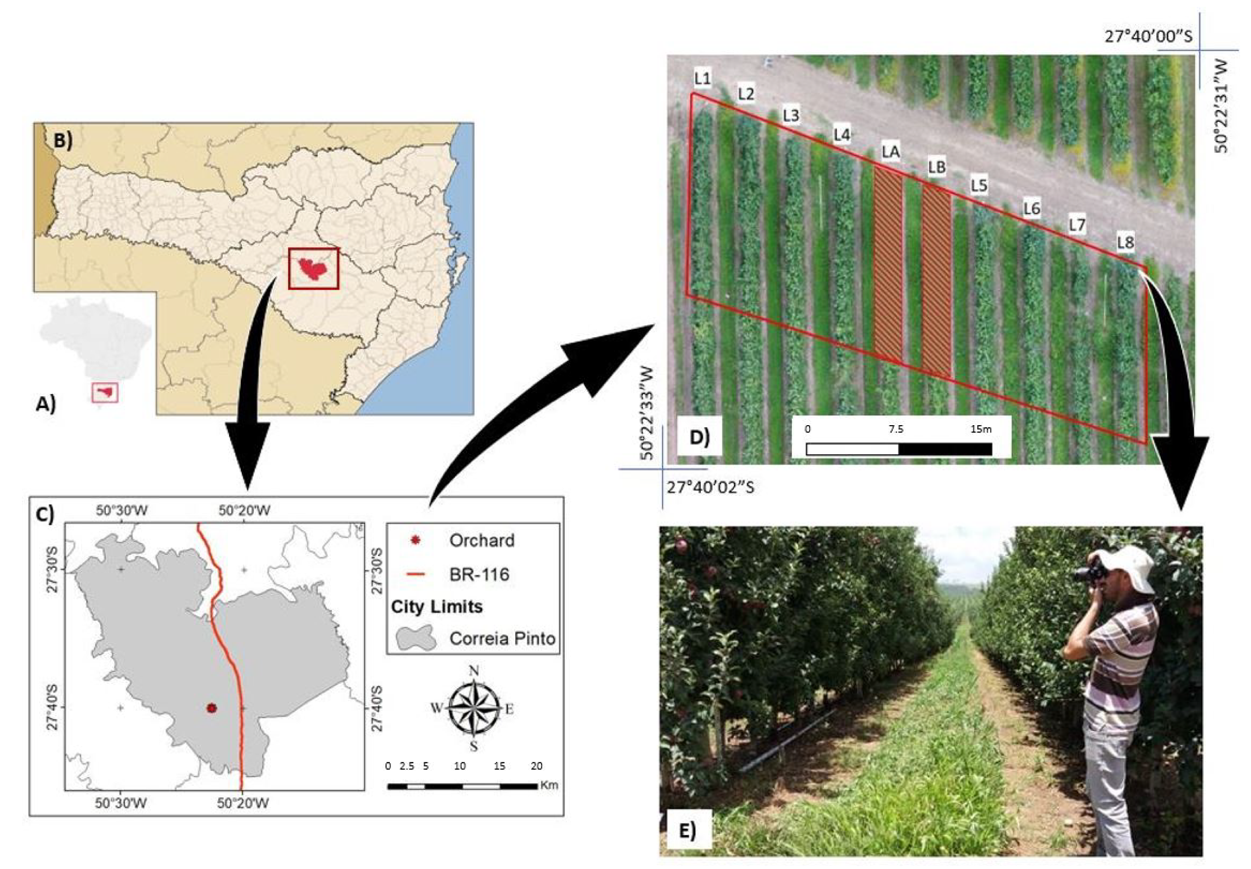
The experiment was conducted in the Correia Pinto municipality, State of Santa Catarina, Brazil, in a commercial orchard (2740′01″ S, 5022′32″ W) (Figure 1A–C). According to the Köppen classification, the climate is subtropical (Cfb) with temperate summers [53].The soil of the region is classified as Inceptisol according to American Soil Taxonomy System [54], which corresponding to Cambissolo (CHa) in the Brazilian Soil Classification System [55]. The relief is relatively flat, and the altitude above sea level is 880 m. The averaged annual accumulated precipitation is 1560 mm, based on the pluviometric records of the Lages station (2750005—INMET), located 15 km from the orchard, in 74 years period (1941–2014) [56]. The precipitation is regularly distributed between the months September to February, with an average of 150 mm per month. The average precipitation from April to June is below 100 mm. Frost events usually occur from April to September.

Figure 1.
Study area within: (A) Brazil context; (B) Santa Catarina State context; (C) Municipality of Correia Pinto and location of the orchard [60]; (D) Aerial view of the sample site and Identification of the samples of the Fuji Suprema rows from L1 to L8, and Gala rows at LA and LB; (E) perspective of the Image acquisition in the orchard during the field survey.
The State of Santa Catarina represents 50% of the Brazilian apple production. Up to 90% of this production comes from orchards with an average size of 10 hectares [57,58]. In general, the owners of these small rural properties have limited resources to invest in management tools and decision support, making the use of close-range and low-cost terrestrial RGB images for automatic apple fruit detection an interesting alternative.
The selected study orchard has 46 ha, and the apple trees were planted in 2009, keeping a spacing of 0.8 × 3.5 m. As a result, a density of 3570 plants·ha is found with an alignment in the planting rows following the N-S orientation. In the analyzed area, two apple cultivars were planted: Fuji Suprema and Gala, and they were planted in rows to be cultivated, keeping a proportion of four rows of Fuji Suprema for two rows of Gala, respectively. This practice is used for facilitating the cross-pollination [59]. The analyzed cultivar was Fuji Suprema, divided by a row of samples identified from L1 to L8 (Figure 1D). The two Gala cultivar rows labeled as LA and LB in the same figure were already harvested when the field surveys were conducted and therefore precluded from further analysis. The targeted surveyed area was not covered with an anti-hail net.
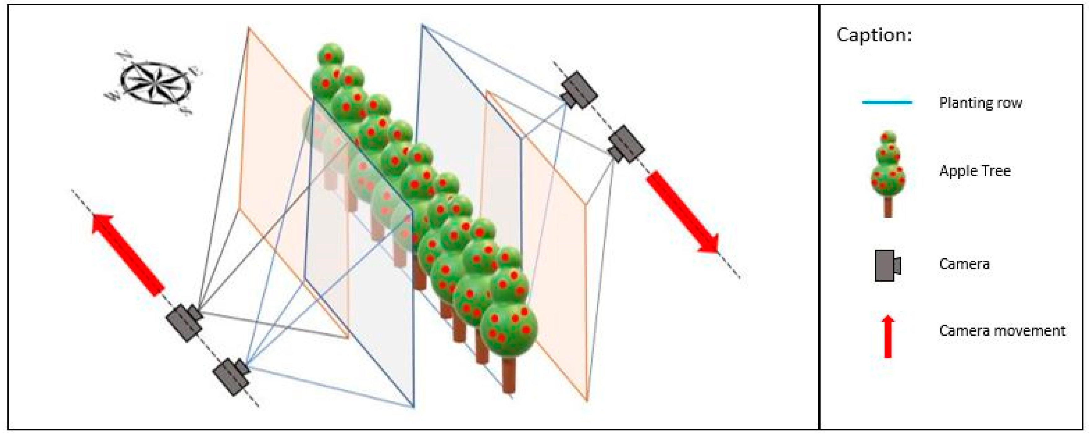
2 To acquire the image dataset, a Canon EOS—T6 camera (Tokyo, Japan, CMOS sensor of 5184 × 3456 pixel (17.9 Mp) and pixel size of 4.3 m) was used with a fixed and nominal focal length of 18 mm. The camera was operated manually, in the portrait position at the operator’s face’s height, with the cameras’ auxiliary flash active (Figure 1E). Figure 2 shows the mode of image acquisition nearly perpendicular at a given planting row. With each image capture, a small step parallel to the planting line was taken, and a new acquisition was then made, similar to the “Stop and Go” mode adopted by Liang et al. [61].

Figure 2.
Graphic scheme of obtaining the images in the Orchard. Overlapping the ground pictures are also shown.
The images were obtained on two dates, first on 29 March and second on 1 April 2019, with variations in the day’s acquisition times. In this period, the apple fruits were near ripe and close to the point of harvesting according to visual inspection of specialists in the field. The cultivar under analysis has a red and uniform color soon after flowering, covering 80% to 100% of the fruit [62].
The acquisition times for each planting line are shown in Table 1, and varied between 11:50 a.m. and 6:20 p.m. local time. No artificial background was adopted, and the natural light varied between cloudy and sunny days. Agricultural management procedures conducted using either agricultural machinery or tractors during a usual working day usually occur at that time interval.

Table 1.
Information on date, beginning and finish time of images acquisitions.
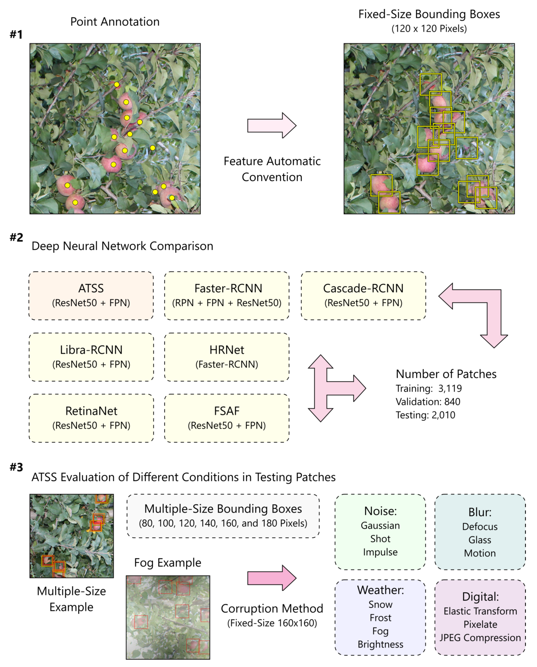
The annotations of the apple fruits were performed manually in the online application VIA (http://www.robots.ox.ac.uk/~vgg/software/via/via-1.0.6.html) (VGG Image Annotator) [63], by specialists. In this procedure, a marking point, annotated in the center of each fruit, was then added. The inspection of each single point was doubled checked by a second specialist. The summarized approach idealized in this study is illustrated in Figure 3 and be summarized into three main steps. The first step (#1), illustrates the dot annotation at the center of each apple fruit and the setting of the bounding box size, with a value fixed of 120. At step (#2), we highlight the state-of-art object detection models used in our work and the distribution of image patches into training, validation, and test set. Step (#3) shows the setting of the bounding box size, whose value range from 80 to 180 with an interval of 20 and four categories (noise, blur, weather, and digital) of the image corruption methods applied in the test set to evaluate the model robustness of the ATSS.

Figure 3.
The workflow for apple-fruit detection divided into three main steps: (#1) annotation process, (#2) image patches distribution into training, validation, and test, and the methods applications and comparison and (#3) image corruption process.
2.2. Object Detection Methods
In the proposed approach to apple-fruit detection, we compared the ATSS [43] method to six popular object detection methods, including Faster-RCNN, Libra-RCNN [49], Cascade-RCNN [50], RetinaNet, Feature Selective Anchor-Free—FSAF [51], and HRNet [52]. We chose these methods for two main reasons: (i) they constitute the state-of-the-art in object detection proposals in the last years; (ii) they cover the main directions of object detection research: two-stage and one-stage, and anchor-based and anchor-free detectors. Below, we briefly describe the main characteristics of each adopted method.
ATSS: Experimental results shown in Reference [43] concluded that an important step in training object detection methods is the choice of positive and negative samples. Therefore, ATSS [43] proposes a new strategy to select samples following objects’ statistical characteristics. For each ground truth g, k anchor boxes whose center is closest to the center of g are selected as positive candidates. Then, the IoU between candidates and g is calculated, obtaining the mean and standard deviation of the IoUs. A threshold is calculated as and used to select final positive candidates whose IoU is greater than or equal to that threshold. The remaining samples are used as negatives. In this work, ATSS has ResNet50 and Feature Pyramid Network (FPN) as a backbone, and anchor boxes are first selected as positive candidates.
Faster-RCNN: The Faster-RCNN [41] is a two-stage CNN that uses the Region Proposal Network (RPN) to generate candidate bounding boxes for each image. The first stage regresses the location of each candidate bounding boxes, and the second stage predicts its class. In this work, we build the FPN on top of the ResNet50 network, as proposed in Reference [64]. This setting brings some improvements in the results to the Faster-RCNN since the ResNet+FPN extract rich semantical features on the images that feed the RPN to help the detector predict the bounding box location betters.
Cascade-RCNN: In training object detection methods, an IoU threshold is set to select positive and negative samples. Despite the promising results, Faster-RCNN uses a fixed IoU threshold of 0.5. A low value for IoU threshold during training can produce noisy detections, while high values can result in overfitting due to the lack of positive samples. To improve this issue, Cascade-RCNN Reference [50] proposes a sequence of detectors with increasing IoU thresholds trained stage by stage. The output of a detector is used to train a subsequent detector. In this way, the final detector receives a superior distribution and produce more quality detections. Following the authors of Reference [50], we have used ResNet50+FPN as a backbone and three cascade detectors with IoUs of 0.5, 0.6, and 0.7, respectively.
Libra-RCNN: Despite the wide variety of object detection methods, most of them follow three stages: (i) proposal of regions, (ii) feature extraction from these regions, and (iii) classification of categories and refinement of bounding boxes. However, the imbalance in these three stages prevents the increase in the overall accuracy. Thus, Libra-RCNN [49] proposes three components to force balancing in the three stages explicitly. In the first stage, the proposed IoU-balanced sampling mines hard samples according to their IoU with the ground-truth uniformly. To reduce the imbalance in the feature extraction, Libra-RCNN proposes the balanced feature pyramid, which resizes the feature maps from the FPN to the same size, calculates the average, and resizes them back to the original size. Finally, balanced L1 loss rebalances the tasks of classification and localization. In this method, we have used ResNet50+FPN as the backbone.
HRNet: The main purpose of the HRNet [52] is to maintain the feature extraction in high-resolution throughout the backbone. HRNet consists of four stages, where the first stage uses high-resolution convolutions. The second, third, and fourth stages are made up of multi-resolution blocks. Each multi-resolution block connects high-to-low resolution convolutions in parallel and fuses multi-scale representations across parallel convolutions. In the end, low-resolution representations are rescaled to high-resolution through bilinear upsampling. In this method, we used HRNet as a backbone and Faster-RCNN heads to detect objects.
RetinaNet: To improve the accuracy of the single-stage object detections with regards to the two-stage methods, the RetinaNet was proposed in Reference [42] to solve the extreme class imbalance. The RetinaNet solves the class imbalance of the positive (foreground) and negative (background) samples by introducing a new loss function named Focal Loss. Since the annotation keeps only the positive samples (ground-truth bounding boxes), the negative samples are obtained during the training after generating candidate-bound boxes that do not match the ground-truth. In this sense, depending on the number of generated candidate bounding boxes, the number of negative samples can be over-represented. To solve this problem, RetinaNet down-weights the loss assigned to well-classified samples (whose probability of ground-truth is above 0.5) and focuses on samples hard to classify. The RetinaNet architecture is composed of a single network with ResNet+FPN as the backbone and two independent subnetworks to regress and classify the bounding boxes. In our experiments, we combine the Resnet50 network with the FPN.
FSAF: This method proposes the feature selective anchor-free (FSAF) module [51] to be applied to single-shot detectors with FPN structure, such as RetinaNet. In such methods, choosing the best level of the pyramid for each object’s training is a complicated task. Thus, FSAF module attaches an anchor-free branch at each level of the pyramid that is trained with online feature selection. We used the RetinaNet with FSAF module, including the ResNet50+FPN as its backbone.
2.3. Proposed Approach
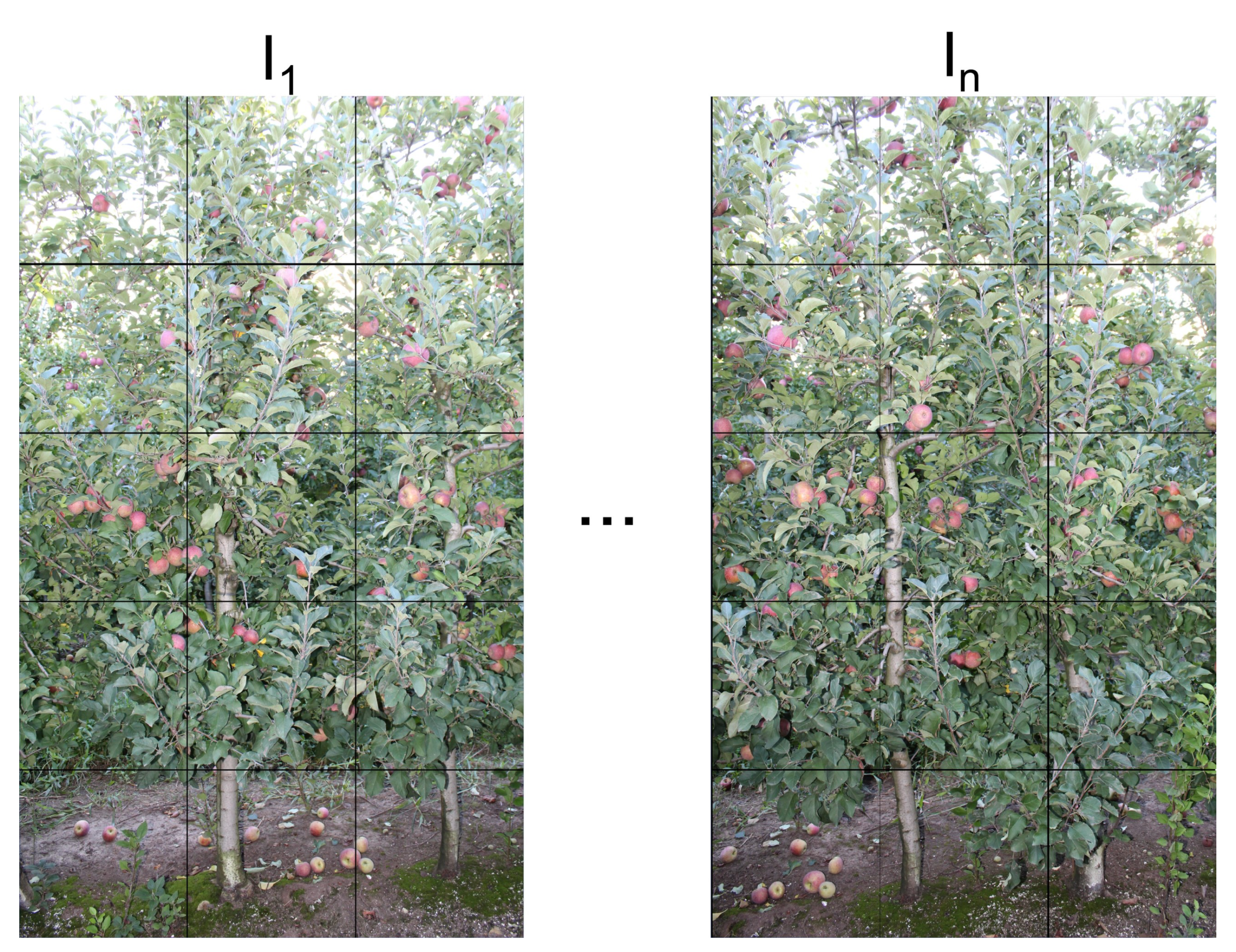
The proposed approach to training the implemented object detection methods can be divided into three steps. The first step is to split the high-resolution images into patches. This division aims to aid the detection of small and/or occluded apples. Given an image, it is divided into non-overlapping patches with size as shown in Figure 4.

Figure 4.
Example of two images and their division into non-overlapping patches.
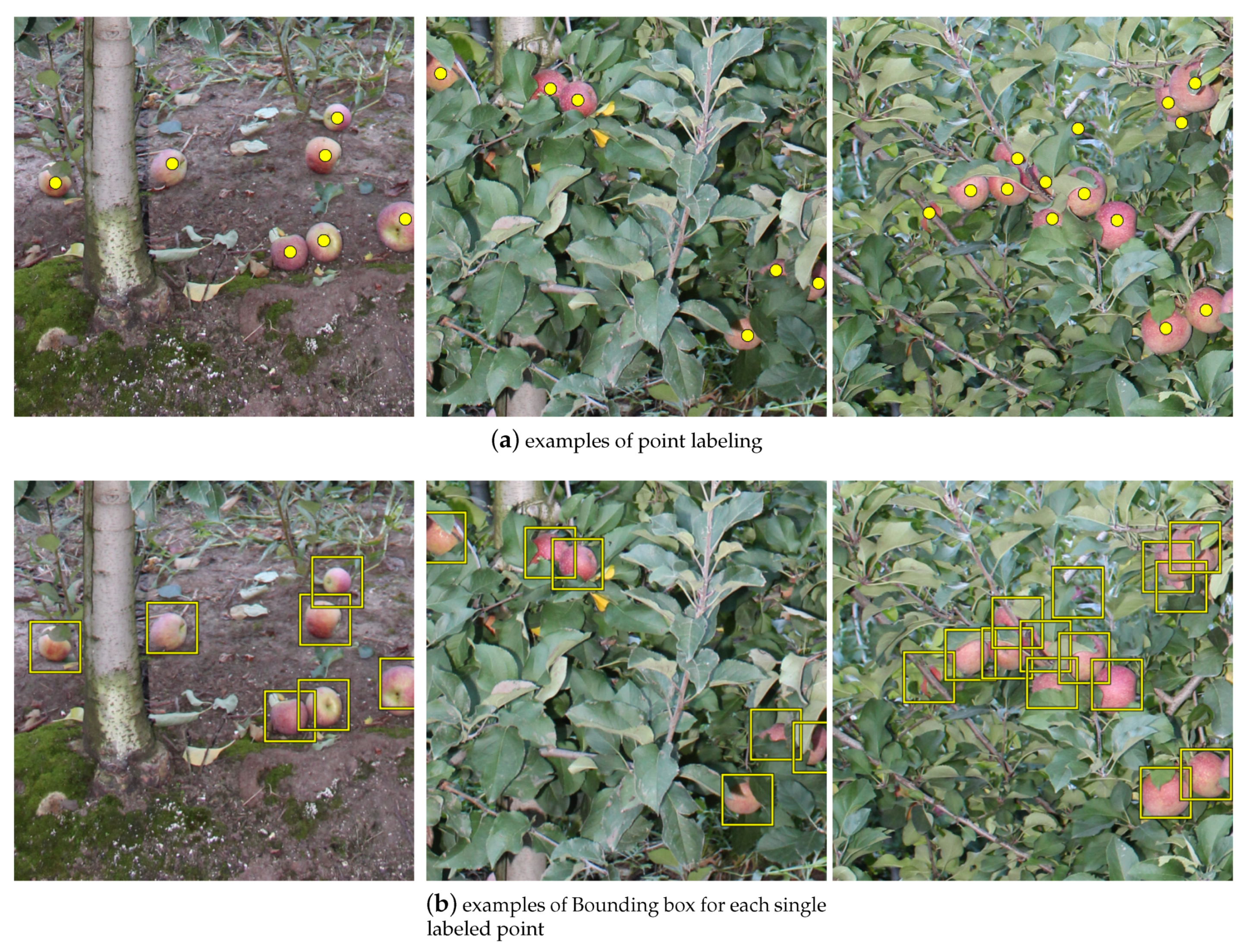
In the second step, the apples were labeled with a point in their center (Figure 5a). The apple fruits over the ground were also marked. This point feature speeds up the labeling process and is essential for labeling a large number of patches. However, these labels are not directly usable in object detection methods that require a bounding box. To work around this problem, we propose to estimate a fixed size bounding box around each labeled point (Figure 5b). This weak labeling is also important to assess how well each bounding box needs to be evaluated in recent methods.

Figure 5.
Subsets of a given RGB image showing some examples of manual labeling with points in the center of the apple fruits (a) and estimation of bounding box with fixed size for each single labeled point (b).
Finally, in the last step, patches and ground-truths were used to train the object detection methods. We then tested the methods described in Section 2.2. Given the trained method, it can be used to detect apples in the test step.
2.4. Experimental Setup
The plantation lines were randomly divided into training, validation and testing sets. Due to the high resolution of the images, they were divided into patches of pixels as described in the previous section. Table 2 shows the division of the dataset with the number of images, patches, and apples in each set.

Table 2.
Plantation lines in the training, validation and test set.
Following the common practice [43], the input patches have been resized to pixels and normalized using mean color values of and variances of . For data augmentation, each input patch was randomly flipped with a probability of 0.5. Given the manually labeled centers, bounding boxes with a fixed size of pixels were first evaluated. Next, we tested different sizes ranging from to pixels.
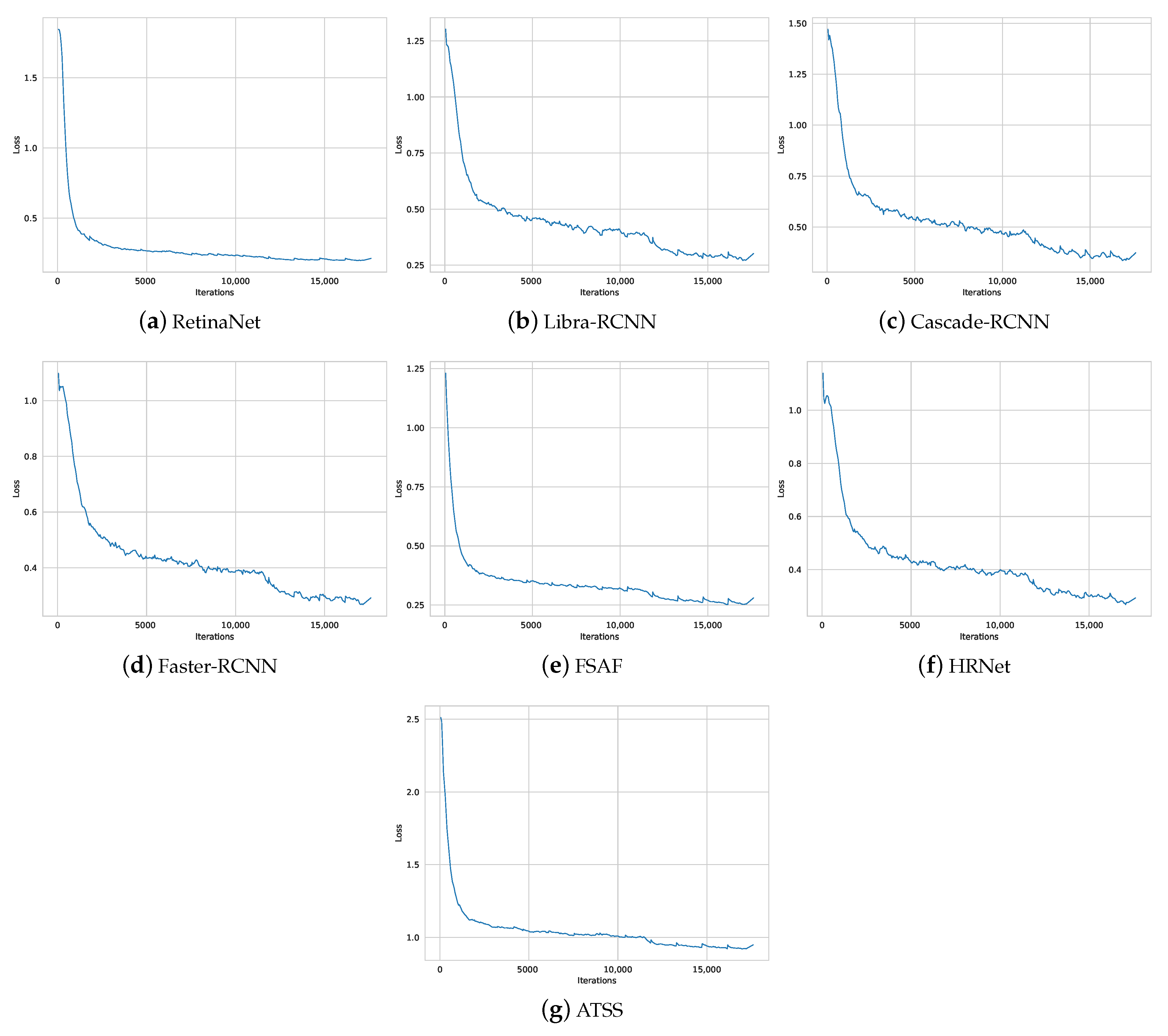
For training, the backbone of the object detection methods was initialized with the pre-trained weights on ImageNet in a strategy known as Transfer Learning. A set of hyper-parameters was fixed for all methods after validation. Faster-RCNN, Libra-RCNN, Cascade-RCNN, and HRNet were trained using SGD optimizer for 17,500 iterations with a learning rate of 0.02, a momentum of 0.9, and a weight decay of 0.0001. RetinaNet, FSAF, and ATSS followed the same hyper-parameters, except that they used an initial learning rate of 0.01 as shown in Table 3. They were also trained with a higher learning rate (0.02), but did not converge properly during training. Figure 6 illustrates the behavior of the loss curve for the methods. We can see that the curve drops dramatically in the first iterations and stabilizes afterward, showing that the training was adequate.

Table 3.
Hyper-parameters of each object detection method.

Figure 6.
Loss curve when training the methods.
As an evaluation metric, we use the average precision (AP) commonly used in object detection with IoU of 0.5. In summary, this metric determines examples as true-positive (TP) when the IoU value is greater than a threshold (0.5 in our experiments) and false-positive (FP) otherwise. The IoU stands for the Intersection Over Union, which is calculated as the overlapping area between the predicted and the ground-truth bounding boxes divided by the union between them. According to this amount of TP and FP examples, the AP is calculated as the area under the precision-recall curve, and its value range from 0 (low) to 1 (high). The precision and recall are calculated according to Equations (1) and (2), respectively.
The model robustness was measured by applying 13 image corruptions type, and three severity levels (SL) per corruption type. As pointed out in Reference [65], these images corruptions are not recommended to be used in training data as a data augmentation toolbox. In this sense, the corruptions were applied only for the images in the test set. The corruptions are distributed in four categories: (i) noise (Gaussian, shot and impulse); (ii) blurs (defocus, glass, and motion); (iii) weather conditions that usually occur in the study area (snow, frost, fog, and brightness); and (iv) digital image processing (elastic transform, pixelate, and JPEG compression). According to Hendrycks et al. [66], we follow the same severity levels. However, in our experiments, only three instead of five levels were considered.
All experiments were performed in a desktop computer with Intel(R) Xeon(R) CPU E3-1270@3.80 GHz, 64 GB memory, and NVIDIA Titan V Graphics Card (5120 Compute Unified Device Architecture—CUDA cores and 12 GB graphics memory). The methods were implemented using mmdetection toolbox (https://github.com/open-mmlab/mmdetection) on the Ubuntu 18.04 operating system.
3. Results and Discussion
3.1. Apple Detection Performance Using Different Object Detection Methods
The summary results of the apple fruit detection methods are shown in Table 4. For each deep learning-based method, AP for each plantation line is presented in addition to its average and standard deviation (std). Experimental results showed that ATSS obtained the highest AP of 0.925(±0.011), followed by HRNet and FSAF. Traditional object detection methods, such as Faster-RCNN and RetinaNet, obtained slightly lower results with AP of 0.918(±0.016) and 0.903(±0.020), respectively. Despite this, all methods showed results above 0.9, which indicates that apple counting automatically is a possible task. Compared to manual counting by a human inspection, automatic counting is much faster, with similar accuracy.

Table 4.
Average precision (AP) of the apple detection methods in three plantation lines of the test set.
The last column of Table 4 shows the estimated number of apples detected by each method in the test set. We can see that ATSS detected approximately 50 more apples than the second best method (HRNet or FSAF). It is important to highlight that this result was obtained in three plantation lines, while the impact on the entire plantation would be much greater. In addition, the financial impact on an automatic harvesting system using ATSS, for example, would be considerable despite the small difference in AP.
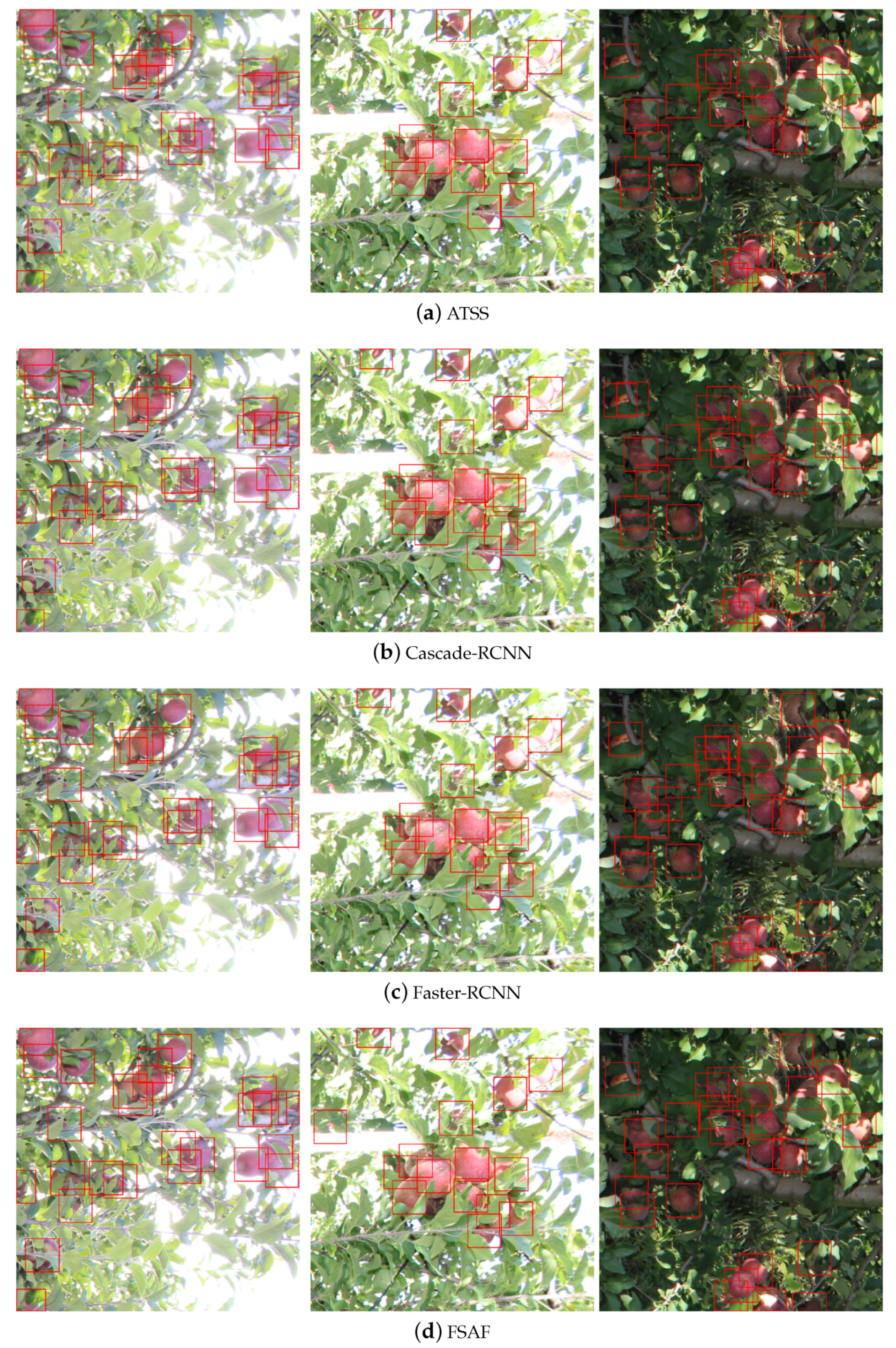
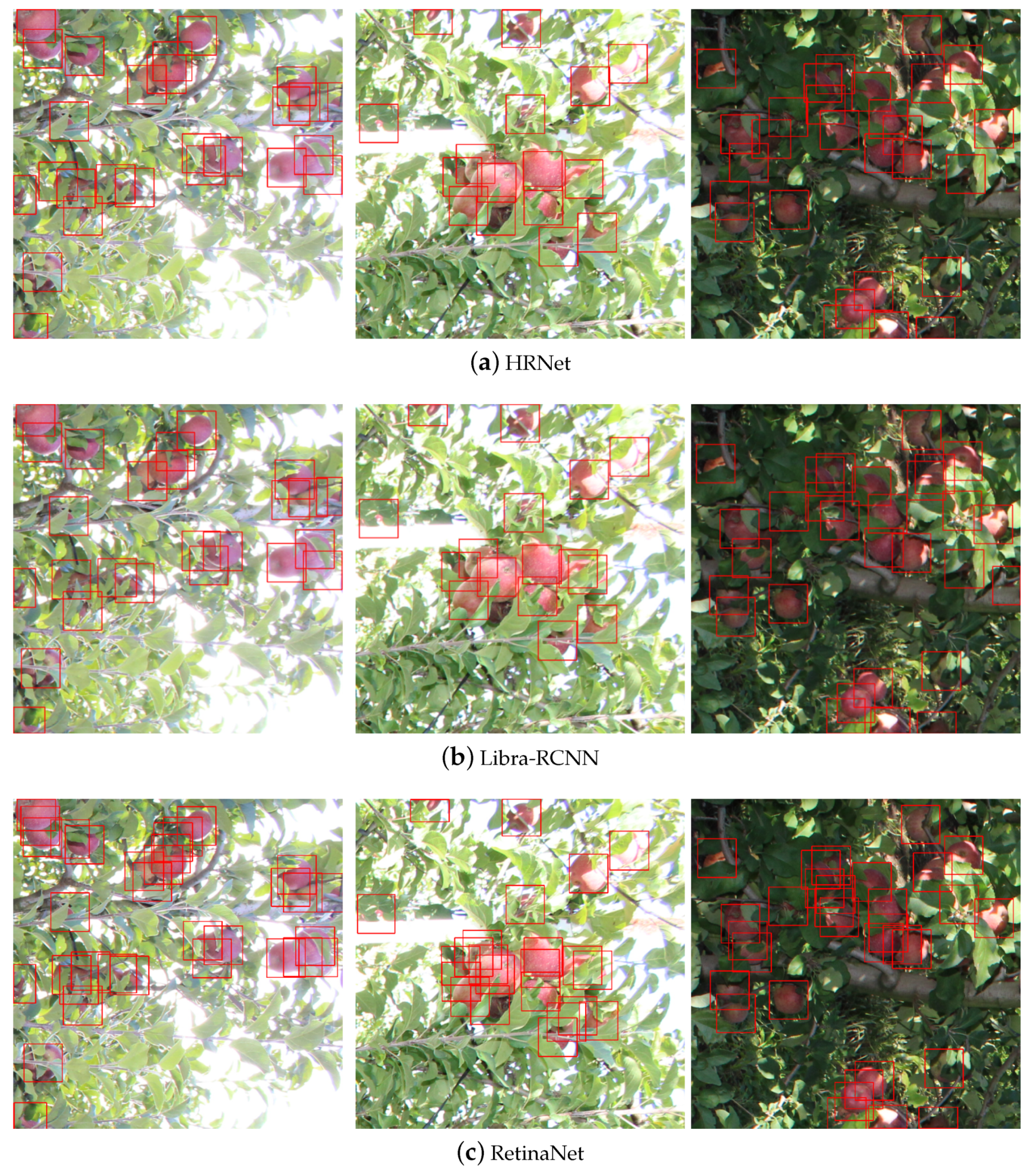
Examples of apple detection are shown in Figure 7 and Figure 8 for all object detection methods. These images presented challenging scenarios with high apple occlusion and different lighting conditions. Occlusion and differences in lighting are probably the most common problems faced by this type of detection, as observed in similar applications [29,30,31]. The accuracy obtained by the ATSS method in our data-set was similar or superior when compared against other tree-fruit detection tasks [67].

Figure 7.
Examples of apple detection using (a) Adaptative Training Sample Selection (ATSS), (b) Cascade-Regions with Convolutional Neural Network (Cascade-RCNN), (c) Faster-Regions with Convolutional Neural Network (Faster-RCNN), and (d) Feature Selective Anchor-Free (FSAF).

Figure 8.
Examples of apple detection using (a) High-Resolution Network (HRNet), (b) Libra-Regions with Convolutional Neural Network (Libra-RCNN), and (c) RetinaNet.
These images are challenging even for humans, who would take considerable time to perform a visual inspection. Despite the challenges imposed on these images, the detection methods presented good visual results, including ATSS (Figure 7a). On the other hand, the lower AP of RetinaNet is generally due to false positives, as shown in Figure 8c.
It is important to highlight that the methods were trained with all bounding boxes of the same size (Table 2). However, the estimated bounding boxes were not all the same size. For example, for Faster-RCNN, the calculated width and height of all predicted bounding boxes in the test set have an average size of 114.60(±15.44) × 114.96(±17.40). The standard deviation, therefore, indicates that there is a variation between the predicted bounding boxes. The bounding boxes average area was 13,233 (±4232.4), indicating the variation between the predicted boxes.
3.2. Influence of the Bounding Box Size
The results of the previous section were obtained with a bounding box size of pixels. In this section, we evaluated the influence of the bounding box size on the ATSS, as it obtained the best results among all of the object detection methods. Table 5 shows the results returned when using sizes from to .

Table 5.
Results of Average Precision for different bounding box (BB) sizes obtained by the ATSS.
Bounding boxes with small size (e.g., pixels) did not achieve good results as they did not cover most of the apple fruit edges. The contrast and the edges of the object are important for the adequate generalization of the methods. On the other hand, large sizes (e.g., ) cause two or more apples to be covered by a single bounding box. Therefore, the methods cannot detect apple fruits individually, especially small ones or in occlusion. The experiments showed that the best result was obtained with a size of pixels.
Despite the challenges imposed by the application (e.g., fruit apples with large occlusion, scales, lighting, agglomeration), the results showed that the AP is high even without labeling a bounding box for each object. Since previous fruit-tree object detection studies [29,31] used different box-sizes as label mainly because of perspective differences in the fruit position, this type of information should be considered, as manual labeling is an intensive and laborious operation.
Here, we demonstrated that, with the ATSS method, when objects have a regular shape, which is generally the case with apples, using a fixed-size bounding box is sufficient to obtain acceptable AP. This, by itself, may facilitate labeling these fruits since the specialist can use a point-type of approach and, later, a fixed size can be adopted by the bounding-box-based methods what implies a significant time reduction.
3.3. Detection at Density Levels
In this section, we evaluated the results of ATSS with a bounding box of size in patches with different numbers of apples (density). Table 6 presents the results for patches with numbers of apples between 0–9, 10–19, ⋯, 30–42. The greater the number of apples in a patch, the greater the challenge in detection.

Table 6.
Results of the ATSS in different apple densities in the patches.
We can see that the method maintains precision around 0.94–0.95 for densities between 0–29 apples. Figure 9 shows examples of detection in patches without apples, for example. This shows that the method is consistent in detecting a few apples to a considerable amount of 29 apples in a single patch. As expected, the method’s precision decreases at the last density level (patches with 30–42 apples). However, the precision is still adequate due to the large amount of apples.

Figure 9.
Examples of patches without apples.
3.4. Robustness against Corruptions
In this section, we evaluated the model robustness of the ATSS with a bounding box of size pixels in different corruptions only for the images in the test set. These corruptions simulate possible conditions to occur in image acquisition in situ, among adverse environmental factors, sensor attitude, and degradation in data recording.
Table 7 and Table 8 shows the results for different corruptions and severity levels. The noise results among the three severity levels (Table 7) indicated a reduction in averaged precision between 2.7% and 11.1% compared to non-corruption values. When considering gaussian and shot noise, the precisions were reduced in the same proportion, while the reduction caused by the impulse noise was higher in the first and second levels. Despite the severity levels of noise corruption, the precision was over 84%.

Table 7.
Average precision for different noises and blurs at three severity levels obtained by ATSS.

Table 8.
Average precision for different weather conditions and digital processing at three severity levels obtained by ATSS.
The reduction in the precision for all the blur components (Table 7) was very similar, showing a slight decrease compared with the non-corruption condition. The reduction values were between 0% and 4.8%. In all three severity levels, the obtained results from motion blur impacted less when compared to those results achieved from defocus and glass. The lowest precision here was caused due to the defocus blur. All results showed precision values above 90%, even considering all the severity levels.
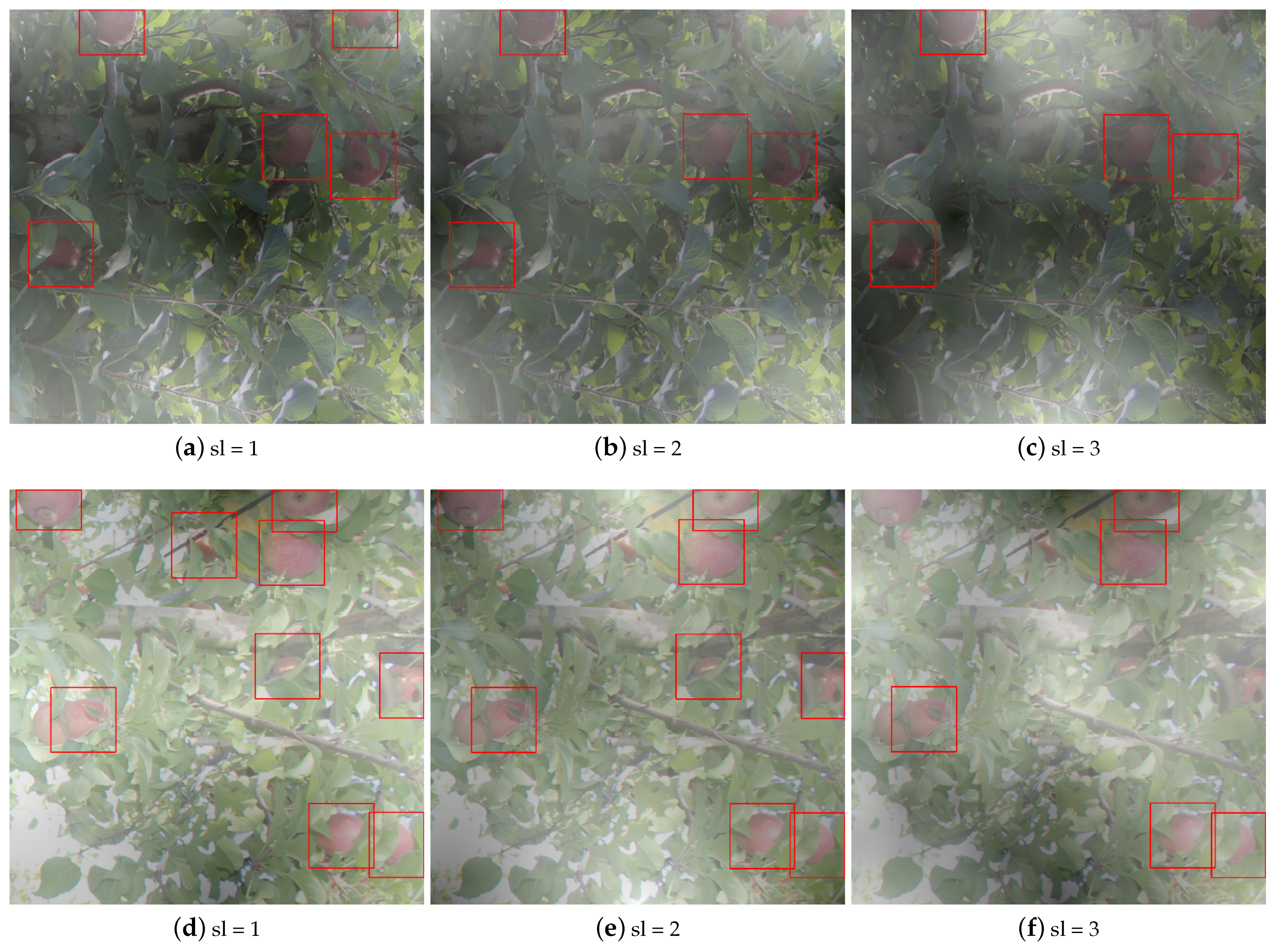
According to the results shown in Table 8, the fog resulted in less precision in the different simulated weather conditions. The precision reductions were approximately 15.5% to 35.5% from the first to the third severity level, respectively. Figure 10 shows the apple detection in two images corrupted by fog. By increasing the severity level of the fog, some apples are not detected. This loss of precision is mainly expected when there are apples with large leaf occlusion.

Figure 10.
Example of two different patches (upper and above rows) with fog (sl stands for severity level).
The brightness implied a slight precision reduction, between 0.5% and 2.4%, compared to the no-corruption condition. In the second severity level, the snow condition achieved the second-worst precision for all weather conditions. The obtained precisions from digital processing, in the elastic transform and pixelate, were near 95% for all severity levels, and the obtained results from JPEG compression were near to 92%. The pixelate showed the best precision results for all severity levels than other digital conditions, with the lowest precision reduction. The JPEG compression precisions reductions were between 1.4% to 3.2% for the severities levels 1 to 3, respectively, compared to the no-corruption condition. In general, the weather condition affected more precision than digital processing.
Previous works [37,39,40] investigated and adapted Faster R-CNN and Yolo-v3 methods. Here, we investigated a novel method based on ATSS, and presented its potential for apple fruit detection. In a general sense, the results indicated that the ATSS-based method slightly outperformed the other deep learning methods, with the best result obtained with a bounding box size of 160 × 160 pixels. The proposed method was robust regarding most of the corruption, except for snow, frost, and fog weather conditions. However, the results remain still satisfactory what implies good accuracy records for apple fruit detection even when RGB pictures are acquired in periods when weather conditions are not that favorable such as frost, fog, and even snow events that are frequent during winter in some areas of the southern Santa Catarina Plateau in southern Brazil.
3.5. Further Research Perspectives
This research made all the close-range and low-cost terrestrial RGB images available, including the annotations. These images can be acquired manually in the field. However, cameras can also be installed in agricultural implements such as sprayers, or even in tractors and autonomous vehicles [68]. This would be interesting to check the applicability of such images in the previous phases or even during the apple fruits’ harvesting. As the inspection process of the apple fruits is performed locally, it is also subjective. Interestingly would be to count fruits that fall in the ground and the impact in the estimation of the final apple fruit production. Another important task is to segment each fruit, which can be performed using a region growing strategy or based on DL instance segmentation methods.
Some orchards with plums and grapes would present similar changes as shown here by apples due to their particular shape and color. Both orchards also used the anti-hail plastic net cover to prevent further damages after the fruit setting until the harvesting period. However, some challenges may particularly occur when dealing with avocado, pear, and feijoa since the typical green color of these fruits is very similar to their leaves green color. These specific fruits would surely require adjustments in this manuscript’s proposed methodology and are also encouraged for further studies. Interestingly, the time demanding and performance of using both the marking point, annotated in the center of each fruit, and a bounding box annotation using bounding boxes is also recommended for completeness of comparisons.
Besides fruit identification, other fruit attributes such as shape, weight, and color are also very relevant information targeted by the market and are recommended for further studies. The addition of quantitative information such as shape could support average fruit weight estimation. Such information would provide better and more realistic fruit production estimates. However, the images must contain the entire apple tree plant what sometimes was not the case due to the tree height. Due to the limited space between the planting lines (i.e., 3.5 m), it is sometimes impossible to cover the entire apple tree in the picture frame. Therefore, camera devices are suggested to be installed at different platform heights in agricultural implements or tractors to overcome this problem. Alternatively, further studies could also explore the possibility of acquiring oblique images or the use of fish-eye lens.
Interestingly, the use of photogrammetric techniques with DL would make it possible to locate the geospatial position of the visible fruits [29], as well as to model their surface. This would enable the individual assessment of the fruit size allowing a more realistic fruit counting. It also eliminates any possibility of counting twice a single fruit eventually in sequential images with overlapping. This may also occur in the images on the backside of the planting row that is also often computed twice [69]. The technique used in this study is encouraged to be analyzed with other fruit varieties that are commercially important in the southern highlands of Brazil, such as pears, grapes, plums, and feijoa [70,71]. Finally, our dataset is available to the general community. The details for accessing the dataset are described in Table A1. It will allow further analysis of the robustness of the reported approaches to counting objects and compares them with forthcoming up-to-date methods.
4. Conclusions
In this study, we proposed an approach based on the ATSS DL method to detect apple fruits using a center points labeling strategy. The method was compared to other state-of-the-art deep learning-based networks, including RetinaNet, Libra R-CNN, Cascade R-CNN, Faster R-CNN, FSAF, and HRNet.
We also evaluated different occlusion conditions and noise corruption in different image sets. The ATSS-based approach outperformed all of the other methods, achieving a maximum average precision of 0.946 with a bounding box size of 160 × 160 pixels. When re-creating the adversity conditions at the time of data acquisition, the approach provided a robust response to most corrupted data, except for snow, frost, and fog weather conditions.
Further studies are suggested with other fruit varieties in which color plays an important role in differentiating them from leaves. Additional fruit attributes such as shape, weight, and color are also important information for determining the market price and are also recommended for future investigations.
To conclude, our study’s relevant contribution is the availability of our current dataset to be publicly accessible. This may help others to evaluate the robustness of their respective approaches to count objects, specifically in fruits with highly-dense conditions.
Author Contributions
Conceptualization, L.J.B., E.M., V.L., J.M.J. and W.N.G.; methodology, L.J.B., W.N.G., J.M.J. and A.A.d.S.; software, D.N.G., J.d.A.S., A.A.d.S., W.N.G. and L.J.B.; formal analysis, L.J.B., V.L., W.N.G., E.M., J.M.J., L.P.O., A.P.M.R., L.R., M.B.S. and S.L.R.N.; resources, L.J.B., E.M. and V.L.; data curation, L.J.B., L.R. and V.L.; writing—original draft preparation, L.J.B., J.M.J., J.d.A.S., L.P.O., W.N.G. and N.V.E.; writing—review and editing, V.L., E.M., D.N.G., A.P.M.R. and A.A.d.S.; and supervision, E.M., J.M.J. and V.L.; project administration, J.A.S.C., J.M.J., M.B.S. and V.L.; and funding acquisition, E.M. and V.L. All authors have read and agreed to the published version of the manuscript.
Funding
This research was partially funded by the Santa Catarina Research Foundation (FAPESC; 2017TR1762, 2019TR816), the Brazilian National Council for Scientific and Technological Development (CNPq; 307689/2013-1, 303279/2018-4, 433783/2018-4, 313887/2018-7, 436863/2018-9, 303559/2019-5, and 304052/2019-1) and the Coordination for the Improvement of Higher Education Personnel (CAPES; Finance Code 001). APC charges of this manuscript were covered by the Remote Sensing 2019 Outstanding Reviewer Award granted to V.L.
Institutional Review Board Statement
Not applicable.
Informed Consent Statement
Not applicable.
Data Availability Statement
The data presented in this study are openly available. The links for downloading the data are provided in Table A1.
Acknowledgments
We would like to thank the State University of Santa Catarina (UDESC), and the Department of Environmental and Sanitation Engineering, for supporting the doctoral dissertation of the first author. We would also like to thank the owner of the study site for allowing us access into the rural property, as well as for their availability and generosity. The authors also acknowledge the computational support of the Federal University of Mato Grosso do Sul (UFMS). Finally, we would like to thank the editors and two reviewers for providing very constructive concerns and suggestions. Such feedback has greatly helped us improve the quality of the manuscript.
Conflicts of Interest
The authors declare no conflict of interest. The funders had no role in the design of the study; in the collection, analyses, or interpretation of data; in the writing of the manuscript, or in the decision to publish the results.
Abbreviations
The following abbreviations are used in this manuscript:
| DL | Deep Learning |
| ATSS | Adaptative Training Sample Selection |
| RGB | Red, Green and Blue |
| R-CNN | Regions with Convolutional Neural Network |
| FSAF | Feature Selective Anchor-Free |
| HRNet | High-Resolution Network |
| UPN | Unsupervised Pre-Trained Networks |
| RNN | Recurrent Neural Networks |
| CNN | Convolutional Neural Network |
| RPA | Remote Piloted Aircraft |
| SVM | Support Vector Machines |
| YOLO | You Only Look Once |
| RGB-D | Depth Camera |
| IoU | Intersection over Union |
| INMET | National Institute of Meteorology |
| CMOS | Complementary Metal Oxide Semiconductor |
| Mp | Megapixel |
| μm | Micrometer |
| VIA | VGG Image Annotator |
| VGG | Visual Geometry Group |
| ResNet | Residual Network |
| FPN | Feature Pyramid Network |
| RPN | Region Proposal Network |
| SGD | Stochastic Gradient Descent |
| AP | Average Precision |
| TP | True Positive |
| FP | False Positive |
| P | Precision |
| R | Recall |
| SL | Severity Levels |
| std | Standard Deviation |
| BB | Bounding Box |
Appendix A

Table A1.
Table with the size of the files to download.
Table A1.
Table with the size of the files to download.
| File (.ZIP) | Plantation Lines | N. of Images | N. of Patches | N. of Apples | Download Size (Gigabyte) | Link |
|---|---|---|---|---|---|---|
| Training | 1, 3, 6, 7 | 208 | 3119 | 29,983 | 4.99 Gb | http://gg.gg/trainingfiles |
| Validation | 4 | 56 | 840 | 7010 | 1.33 Gb | http://gg.gg/validationfiles |
| Test_L2 | 2 | 50 | 750 | 16,466 | 1.21 Gb | http://gg.gg/L2test |
| Test_L5 | 5 | 44 | 660 | 1.09 Gb | http://gg.gg/L5test | |
| Test_L8 | 8 | 40 | 600 | 1.02 Gb | http://gg.gg/L8test | |
| Total | 8 Lines | 398 | 5969 | 53,459 | 9.64 Gb | http://gg.gg/totalfiles |
References
- Dian Bah, M.; Hafiane, A.; Canals, R. Deep learning with unsupervised data labeling for weed detection in line crops in UAV images. Remote Sens. 2018, 10, 1690. [Google Scholar] [CrossRef]
- Kamilaris, A.; Prenafeta-Boldú, F.X. Deep learning in agriculture: A survey. Comput. Electron. Agric. 2018, 147, 70–90. [Google Scholar] [CrossRef]
- Tu, S.; Pang, J.; Liu, H.; Zhuang, N.; Chen, Y.; Zheng, C.; Wan, H.; Xue, Y. Passion fruit detection and counting based on multiple scale faster R-CNN using RGB-D images. Precision Agric. 2020, 21, 1072–1091. [Google Scholar] [CrossRef]
- Chen, J.; Li, F.; Wang, R.; Fan, Y.; Raza, M.A.; Liu, Q.; Wang, Z.; Cheng, Y.; Wu, X.; Yang, F.; et al. Estimation of nitrogen and carbon content from soybean leaf reflectance spectra using wavelet analysis under shade stress. Comput. Electron. Agric. 2019, 156, 482–489. [Google Scholar] [CrossRef]
- Hasan, M.M.; Chopin, J.P.; Laga, H.; Miklavcic, S.J. Detection and analysis of wheat spikes using Convolutional Neural Networks. Plant Methods 2018, 14, 1–13. [Google Scholar] [CrossRef]
- Hunt, M.L.; Blackburn, G.A.; Carrasco, L.; Redhead, J.W.; Rowland, C.S. High resolution wheat yield mapping using Sentinel-2. Remote Sens. Environ. 2019, 233, 111410. [Google Scholar] [CrossRef]
- Salamí, E.; Gallardo, A.; Skorobogatov, G.; Barrado, C. On-the-fly olive tree counting using a UAS and cloud services. Remote Sens. 2019, 11, 316. [Google Scholar] [CrossRef]
- Ball, J.E.; Anderson, D.T.; Sr, C.S.C. Comprehensive survey of deep learning in remote sensing: Theories, tools, and challenges for the community. J. Appl. Remote Sens. 2017, 11, 1–54. [Google Scholar] [CrossRef]
- Schmidhuber, J. Deep Learning in neural networks: An overview. Neural Netw. 2015, 61, 85–117. [Google Scholar] [CrossRef]
- Deng, L.; Mao, Z.; Li, X.; Hu, Z.; Duan, F.; Yan, Y. UAV-based multispectral remote sensing for precision agriculture: A comparison between different cameras. ISPRS J. Photogramm. Remote Sens. 2018, 146, 124–136. [Google Scholar] [CrossRef]
- Meng, L.; Peng, Z.; Zhou, J.; Zhang, J.; Lu, Z.; Baumann, A.; Du, Y. Real-Time Detection of Ground Objects Based on Unmanned Aerial Vehicle Remote Sensing with Deep Learning: Application in Excavator Detection for Pipeline Safety. Remote Sens. 2020, 12, 182. [Google Scholar] [CrossRef]
- Zhang, X.; Han, L.; Han, L.; Zhu, L. How Well Do Deep Learning-Based Methods for Land Cover Classification and Object Detection Perform on High Resolution Remote Sensing Imagery? Remote Sens. 2020, 12, 417. [Google Scholar] [CrossRef]
- Yuan, Q.; Shen, H.; Li, T.; Li, Z.; Li, S.; Jiang, Y.; Xu, H.; Tan, W.; Yang, Q.; Wang, J.; et al. Deep learning in environmental remote sensing: Achievements and challenges. Remote Sens. Environ. 2020, 241, 111716. [Google Scholar] [CrossRef]
- Chaudhuri, U.; Banerjee, B.; Bhattacharya, A.; Datcu, M. CMIR-NET: A deep learning based model for cross-modal retrieval in remote sensing. Pattern Recognit. Lett. 2020, 131, 456–462. [Google Scholar] [CrossRef]
- Osco, L.P.; dos Santos de Arruda, M.; Marcato Junior, J.; da Silva, N.B.; Ramos, A.P.M.; Moryia, É.A.S.; Imai, N.N.; Pereira, D.R.; Creste, J.E.; Matsubara, E.T.; et al. A convolutional neural network approach for counting and geolocating citrus-trees in UAV multispectral imagery. ISPRS J. Photogramm. Remote Sens. 2020, 160, 97–106. [Google Scholar] [CrossRef]
- Lobo Torres, D.; Queiroz Feitosa, R.; Nigri Happ, P.; Elena Cué La Rosa, L.; Marcato Junior, J.; Martins, J.; Olã Bressan, P.; Gonçalves, W.N.; Liesenberg, V. Applying Fully Convolutional Architectures for Semantic Segmentation of a Single Tree Species in Urban Environment on High Resolution UAV Optical Imagery. Sensors 2020, 20, 563. [Google Scholar] [CrossRef]
- Zhu, L.; Huang, L.; Fan, L.; Huang, J.; Huang, F.; Chen, J.; Zhang, Z.; Wang, Y. Landslide Susceptibility Prediction Modeling Based on Remote Sensing and a Novel Deep Learning Algorithm of a Cascade-Parallel Recurrent Neural Network. Sensors 2020, 20, 1576. [Google Scholar] [CrossRef]
- Castro, W.; Marcato Junior, J.; Polidoro, C.; Osco, L.P.; Gonçalves, W.; Rodrigues, L.; Santos, M.; Jank, L.; Barrios, S.; Valle, C.; et al. Deep Learning Applied to Phenotyping of Biomass in Forages with UAV-Based RGB Imagery. Sensors 2020, 20, 4802. [Google Scholar] [CrossRef]
- Lecun, Y.; Bengio, Y.; Hinton, G. Deep learning. Nature 2015, 521, 436–444. [Google Scholar] [CrossRef]
- Khamparia, A.; Singh, K.M. A systematic review on deep learning architectures and applications. Expert Syst. 2019, 36, 1–22. [Google Scholar] [CrossRef]
- Li, K.; Wan, G.; Cheng, G.; Meng, L.; Han, J. Object detection in optical remote sensing images: A survey and a new benchmark. ISPRS J. Photogramm. Remote Sens. 2020, 159, 296–307. [Google Scholar] [CrossRef]
- Apolo-Apolo, O.; Martínez-Guanter, J.; Egea, G.; Raja, P.; Pérez-Ruiz, M. Deep learning techniques for estimation of the yield and size of citrus fruits using a UAV. Eur. J. Agron. 2020, 115, 126030. [Google Scholar] [CrossRef]
- Apolo-Apolo, O.E.; Pérez-Ruiz, M.; Martínez-Guanter, J.; Valente, J. A Cloud-Based Environment for Generating Yield Estimation Maps From Apple Orchards Using UAV Imagery and a Deep Learning Technique. Front. Plant Sci. 2020, 11, 1086. [Google Scholar] [CrossRef] [PubMed]
- Veeranampalayam Sivakumar, A.N.; Li, J.; Scott, S.; Psota, E.J.; Jhala, A.; Luck, J.D.; Shi, Y. Comparison of Object Detection and Patch-Based Classification Deep Learning Models on Mid- to Late-Season Weed Detection in UAV Imagery. Remote Sens. 2020, 12, 2136. [Google Scholar] [CrossRef]
- Li, W.; Fu, H.; Yu, L.; Cracknell, A. Deep Learning Based Oil Palm Tree Detection and Counting for High-Resolution Remote Sensing Images. Remote Sens. 2016, 9, 22. [Google Scholar] [CrossRef]
- Csillik, O.; Cherbini, J.; Johnson, R.; Lyons, A.; Kelly, M. Identification of Citrus Trees from Unmanned Aerial Vehicle Imagery Using Convolutional Neural Networks. Drones 2018, 2, 39. [Google Scholar] [CrossRef]
- Habaragamuwa, H.; Ogawa, Y.; Suzuki, T.; Shiigi, T.; Ono, M.; Kondo, N. Detecting greenhouse strawberries (mature and immature), using deep convolutional neural network. Eng. Agric. Environ. Food 2018, 11, 127–138. [Google Scholar] [CrossRef]
- Kirk, R.; Cielniak, G.; Mangan, M. L*a*b*Fruits: A rapid and robust outdoor fruit detection system combining bio-inspired features with one-stage deep learning networks. Sensors 2020, 20, 275. [Google Scholar] [CrossRef]
- Liu, X.; Chen, S.W.; Aditya, S.; Sivakumar, N.; Dcunha, S.; Qu, C.; Taylor, C.J.; Das, J.; Kumar, V. Robust Fruit Counting: Combining Deep Learning, Tracking, and Structure from Motion. In Proceedings of the IEEE/RSJ International Conference on Intelligent Robots and Systems (IROS), Madrid, Spain, 1–5 October 2018; pp. 1045–1052. [Google Scholar] [CrossRef]
- Bargoti, S.; Underwood, J.P. Image Segmentation for Fruit Detection and Yield Estimation in Apple Orchards. J. Field Robot. 2017, 34, 1039–1060. [Google Scholar] [CrossRef]
- Kestur, R.; Meduri, A.; Narasipura, O. MangoNet: A deep semantic segmentation architecture for a method to detect and count mangoes in an open orchard. Eng. Appl. Artif. Intell. 2019, 77, 59–69. [Google Scholar] [CrossRef]
- Koirala, A.; Walsh, K.B.; Wang, Z.; McCarthy, C. Deep learning—Method overview and review of use for fruit detection and yield estimation. Comput. Electron. Agric. 2019, 162, 219–234. [Google Scholar] [CrossRef]
- Dias, P.A.; Tabb, A.; Medeiros, H. Apple flower detection using deep convolutional networks. Comput. Ind. 2018, 99, 17–28. [Google Scholar] [CrossRef]
- Wu, D.; Lv, S.; Jiang, M.; Song, H. Using channel pruning-based YOLO v4 deep learning algorithm for the real-time and accurate detection of apple flowers in natural environments. Comput. Electron. Agric. 2020, 178, 105742. [Google Scholar] [CrossRef]
- Jiang, P.; Chen, Y.; Liu, B.; He, D.; Liang, C. Real-Time Detection of Apple Leaf Diseases Using Deep Learning Approach Based on Improved Convolutional Neural Networks. IEEE Access 2019, 7, 59069–59080. [Google Scholar] [CrossRef]
- Wang, D.; Li, C.; Song, H.; Xiong, H.; Liu, C.; He, D. Deep Learning Approach for Apple Edge Detection to Remotely Monitor Apple Growth in Orchards. IEEE Access 2020, 8, 26911–26925. [Google Scholar] [CrossRef]
- Tian, Y.; Yang, G.; Wang, Z.; Wang, H.; Li, E.; Liang, Z. Apple detection during different growth stages in orchards using the improved YOLO-V3 model. Comput. Electron. Agric. 2019, 157, 417–426. [Google Scholar] [CrossRef]
- Kang, H.; Chen, C. Fast implementation of real-time fruit detection in apple orchards using deep learning. Comput. Electron. Agric. 2020, 168, 105108. [Google Scholar] [CrossRef]
- Gené-Mola, J.; Vilaplana, V.; Rosell-Polo, J.R.; Morros, J.R.; Ruiz-Hidalgo, J.; Gregorio, E. Multi-modal deep learning for Fuji apple detection using RGB-D cameras and their radiometric capabilities. Comput. Electron. Agric. 2019, 162, 689–698. [Google Scholar] [CrossRef]
- Gao, F.; Fu, L.; Zhang, X.; Majeed, Y.; Li, R.; Karkee, M.; Zhang, Q. Multi-class fruit-on-plant detection for apple in SNAP system using Faster R-CNN. Comput. Electron. Agric. 2020, 176, 105634. [Google Scholar] [CrossRef]
- Ren, S.; He, K.; Girshick, R.; Sun, J. Faster R-CNN: Towards Real-Time Object Detection with Region Proposal Networks. arXiv 2015, arXiv:1506.01497. [Google Scholar] [CrossRef]
- Lin, T.Y.; Goyal, P.; Girshick, R.; He, K.; Dollár, P. Focal Loss for Dense Object Detection. arXiv 2017, arXiv:1708.02002. [Google Scholar]
- Zhang, S.; Chi, C.; Yao, Y.; Lei, Z.; Li, S.Z. Bridging the Gap Between Anchor-based and Anchor-free Detection via Adaptive Training Sample Selection. In Proceedings of the IEEE/CVF Conference on Computer Vision and Pattern Recognition CVPR, Seattle, WA, USA, 13–19 June 2020. [Google Scholar] [CrossRef]
- Srivastava, L.M. CHAPTER 17—Fruit Development and Ripening. In Plant Growth and Development; Srivastava, L.M., Ed.; Academic Press: San Diego, CA, USA, 2002; pp. 413–429. [Google Scholar] [CrossRef]
- Mészáros, M.; Bělíková, H.; Čonka, P.; Náměstek, J. Effect of hail nets and fertilization management on the nutritional status, growth and production of apple trees. Sci. Hortic. 2019, 255, 134–144. [Google Scholar] [CrossRef]
- Brglez Sever, M.; Tojnko, S.; Breznikar, A.; Skendrović Babojelić, M.; Ivančič, A.; Sirk, M.; Unuk, T. The influence of differently coloured anti-hail nets and geomorphologic characteristics on microclimatic and light conditions in apple orchards. J. Cent. Eur. Agric. 2020, 21, 386–397. [Google Scholar] [CrossRef]
- Bosco, L.C.; Bergamaschi, H.; Cardoso, L.S.; Paula, V.A.d.; Marodin, G.A.B.; Brauner, P.C. Microclimate alterations caused by agricultural hail net coverage and effects on apple tree yield in subtropical climate of Southern Brazil. Bragantia 2018, 77, 181–192. [Google Scholar] [CrossRef]
- Bosco, L.C.; Bergamaschi, H.; Marodin, G.A. Solar radiation effects on growth, anatomy, and physiology of apple trees in a temperate climate of Brazil. Int. J. Biometeorol. 2020, 1969–1980. [Google Scholar] [CrossRef]
- Pang, J.; Chen, K.; Shi, J.; Feng, H.; Ouyang, W.; Lin, D. Libra R-CNN: Towards Balanced Learning for Object Detection. In Proceedings of the 2019 IEEE/CVF Conference on Computer Vision and Pattern Recognition (CVPR), Long Beach, CA, USA, 15–20 June 2019; pp. 821–830. [Google Scholar] [CrossRef]
- Cai, Z.; Vasconcelos, N. Cascade R-CNN: Delving Into High Quality Object Detection. In Proceedings of the 2018 IEEE Conference on Computer Vision and Pattern Recognition, CVPR 2018, Salt Lake City, UT, USA, 18–22 June 2018; IEEE Computer Society: Washington, DC, USA, 2018; pp. 6154–6162. [Google Scholar] [CrossRef]
- Zhu, C.; He, Y.; Savvides, M. Feature Selective Anchor-Free Module for Single-Shot Object Detection. In Proceedings of the 2019 IEEE/CVF Conference on Computer Vision and Pattern Recognition (CVPR), Long Beach, CA, USA, 15–20 June 2019; pp. 840–849. [Google Scholar] [CrossRef]
- Wang, J.; Sun, K.; Cheng, T.; Jiang, B.; Deng, C.; Zhao, Y.; Liu, D.; Mu, Y.; Tan, M.; Wang, X.; et al. Deep High-Resolution Representation Learning for Visual Recognition. IEEE Trans. Pattern Anal. Mach. Intell. 2020, 1. [Google Scholar] [CrossRef]
- Alvares, C.A.; Stape, J.L.; Sentelhas, P.C.; de Moraes Gonçalves, J.L.; Sparovek, G. Köppen’s climate classification map for Brazil. Meteorol. Z. 2013, 22, 711–728. [Google Scholar] [CrossRef]
- Soil Survey Staff. Soil Taxonomy: A Basic System of Soil Classification for Making and Interpreting Soil Surveys, 2nd ed.; Natural Resources Conservation Service, USDA: Washington, DC, USA, 1999; Volume 436. [Google Scholar]
- dos Santos, H.G.; Jacomine, P.K.T.; Dos Anjos, L.; De Oliveira, V.; Lumbreras, J.F.; Coelho, M.R.; De Almeida, J.; de Araujo Filho, J.; De Oliveira, J.; Cunha, T.J.F. Sistema Brasileiro de Classificação de Solos; Embrapa: Brasília, Brazil, 2018. [Google Scholar]
- National Water Agency (ANA). HIDROWEB V3.1.1—Séries Históricas de Estações. Available online: http://www.snirh.gov.br/hidroweb/serieshistoricas (accessed on 2 November 2020).
- Bittencourt, C.C.; Barone, F.M. A cadeia produtiva da maçã em Santa Catarina: Competitividade segundo produção e packing house. Rev. Admin. Pública 2011, 45, 1199–1222. [Google Scholar] [CrossRef][Green Version]
- Brazilian Institute of Geography and Statistics (IBGE). Censo Agropecuário 2017: Resultados Definitivos; IBGE: Rio de Janeiro, Brazil, 2019. [Google Scholar]
- Denardi, F.; Kvitschal, M.V.A.c.; Hawerroth, M.C. A brief history of the forty-five years of the Epagri apple breeding program in Brazil. Crop. Breed. Appl. Biotechnol. 2019, 19, 347–355. [Google Scholar] [CrossRef]
- Brazilian Institute of Geography and Statistics (IBGE). Geosciences: Continuos Catographic Bases. Available online: https://www.ibge.gov.br/geociencias/cartas-e-mapas/bases-cartograficas-continuas/15807-estados.html?=&t=sobre (accessed on 20 April 2020).
- Liang, X.; Jaakkola, A.; Wang, Y.; Hyyppä, J.; Honkavaara, E.; Liu, J.; Kaartinen, H. The use of a hand-held camera for individual tree 3D mapping in forest sample plots. Remote Sens. 2014, 6, 6587–6603. [Google Scholar] [CrossRef]
- Petri, J.; Denardi, F.; SUZUKI, A.E. 405-Fuji Suprema: Nova cultivar de macieira. Agropecu. Catarin. Florianópolis 1997, 10, 48–50. [Google Scholar]
- Dutta, A.; Zisserman, A. The VIA Annotation Software for Images, Audio and Video. In Proceedings of the 27th ACM International Conference on Multimedia (MM ’19), Nice, France, 21–25 October 2019; ACM: New York, NY, USA, 2019. [Google Scholar] [CrossRef]
- Lin, T.Y.; Dollár, P.; Girshick, R.; He, K.; Hariharan, B.; Belongie, S. Feature Pyramid Networks for Object Detection. arXiv 2017, arXiv:1612.03144. [Google Scholar]
- Michaelis, C.; Mitzkus, B.; Geirhos, R.; Rusak, E.; Bringmann, O.; Ecker, A.S.; Bethge, M.; Brendel, W. Benchmarking Robustness in Object Detection: Autonomous Driving when Winter is Coming. arXiv 2020, arXiv:1907.07484. [Google Scholar]
- Hendrycks, D.; Dietterich, T. Benchmarking Neural Network Robustness to Common Corruptions and Perturbations. In Proceedings of the International Conference on Learning Representations, New Orleans, LA, USA, 6–9 May 2019. [Google Scholar]
- Koirala, A.; Walsh, K.B.; Wang, Z.; McCarthy, C. Deep learning for real-time fruit detection and orchard fruit load estimation: Benchmarking of ‘MangoYOLO’. Precis. Agric. 2019, 20, 1107–1135. [Google Scholar] [CrossRef]
- Underwood, J.P.; Hung, C.; Whelan, B.; Sukkarieh, S. Mapping almond orchard canopy volume, flowers, fruit and yield using lidar and vision sensors. Comput. Electron. Agric. 2016, 130, 83–96. [Google Scholar] [CrossRef]
- Häni, N.; Roy, P.; Isler, V. A comparative study of fruit detection and counting methods for yield mapping in apple orchards. J. Field Robot. 2020, 37, 263–282. [Google Scholar] [CrossRef]
- Fachinello, J.A.C.; Pasa, M.d.S.; Schmtiz, J.D.; Betemps, D.A.L. Situação e perspectivas da fruticultura de clima temperado no Brasil. Rev. Bras. Frutic. 2011, 33, 109–120. [Google Scholar] [CrossRef]
- Schotsmans, W.; East, A.; Thorp, G.; Woolf, A. 6—Feijoa (Acca sellowiana [Berg] Burret). In Postharvest Biology and Technology of Tropical and Subtropical Fruits; Yahia, E.M., Ed.; Woodhead Publishing Series in Food Science, Technology and Nutrition; Woodhead Publishing: Cambridge, UK, 2011; pp. 15–133, 134e–135e. [Google Scholar] [CrossRef]
Publisher’s Note: MDPI stays neutral with regard to jurisdictional claims in published maps and institutional affiliations. |
© 2020 by the authors. Licensee MDPI, Basel, Switzerland. This article is an open access article distributed under the terms and conditions of the Creative Commons Attribution (CC BY) license (http://creativecommons.org/licenses/by/4.0/).

