Article

An Adversarial Generative Network for Crop Classification from Remote Sensing Timeseries Images

School of Geography and Information Engineering, China University of Geosciences, Wuhan 430074, China
*
Author to whom correspondence should be addressed.
Remote Sens. 2021, 13(1), 65; https://doi.org/10.3390/rs13010065
Submission received: 29 October 2020 / Revised: 20 December 2020 / Accepted: 22 December 2020 / Published: 26 December 2020

Abstract

:
Due to the increasing demand for the monitoring of crop conditions and food production, it is a challenging and meaningful task to identify crops from remote sensing images. The state-of the-art crop classification models are mostly built on supervised classification models such as support vector machines (SVM), convolutional neural networks (CNN), and long- and short-term memory neural networks (LSTM). Meanwhile, as an unsupervised generative model, the adversarial generative network (GAN) is rarely used to complete classification tasks for agricultural applications. In this work, we propose a new method that combines GAN, CNN, and LSTM models to classify crops of corn and soybeans from remote sensing time-series images, in which GAN’s discriminator was used as the final classifier. The method is feasible on the condition that the training samples are small, and it fully takes advantage of spectral, spatial, and phenology features of crops from satellite data. The classification experiments were conducted on crops of corn, soybeans, and others. To verify the effectiveness of the proposed method, comparisons with models of SVM, SegNet, CNN, LSTM, and different combinations were also conducted. The results show that our method achieved the best classification results, with the Kappa coefficient of 0.7933 and overall accuracy of 0.86. Experiments in other study areas also demonstrate the extensibility of the proposed method.

1. Introduction

An in-depth understanding of crop types and its corresponding cultivated areas in national agricultural zones is necessary for agricultural monitoring and food security assessment [1], and contributes to the formulation and implementation of relevant policies. Modern earth observation (EO) programs can generate a large amount of remote sensing data, recording the characteristics of electromagnetic waves reflected by ground objects [2], and satellite remote sensing is widely used to obtain vegetation phenological characteristics [3]. Each feature has a unique spectral characteristic, which varies slightly with environmental factors, the accuracy of the sensing device, etc. The effective combination of different sensor sources [4,5], wavebands, and time-stamped remote sensing images provides more comprehensive feature information about crops. Therefore, it is a feasible and meaningful study to explore the classification of crops based on remote sensing images.
Traditional remote sensing-based image classification algorithms of machine learning are gradually being used in the classification [6] and recognition of remote sensing images. These algorithms can be divided into unsupervised and supervised categories [7]. The former contains algorithms such as K-means and ISODATA clustering. However, with the demand for agriculture classification based on complex terrain increasing gradually, those algorithms can no longer meet the accuracy of remote sensing image classification [2]. The latter contains maximum likelihood, minimum distance, and support vector machine (SVM). At this stage, SVM [8] has been widely used in remote sensing image classification, while some problems also appeared. For example, SVM has a greater probability of leakage and misallocation when the sample size is large [9].
Deep learning, referring to deep neural networks, is a kind of machine learning algorithm and has been widely used due to its powerful feature extraction and data expression ability [10]. In recent years, the recognition rate of deep learning on most traditional recognition tasks has increased significantly [11]. A large number of studies have shown that deep learning can extract features from remote sensing images, and improve the classification accuracy [12]. The mainstream deep learning models, including deep belief network (DBN) [13], convolutional neural network (CNN) [14], stack autoencoders (SAE) [15], and recurrent neural network (RNN) [16], have been successfully used in applications of remote sensing-based classification in most cases. In particular, aiming at the phenomenon of “same matter and different spectrum” in remote sensing images, Wu and Yang [17] proposed recording spatial information combined with spectral information and used DBN to complete high-precision classification. Cao et al. [18] proposed an active deep learning method combining active learning and deep learning to train the CNN to classify on the hyperspectral image, which achieves better performance with fewer marker samples than traditional hyperspectral imagery (HSI) classification algorithms. Hsieh and Kiang [19] compared and validated the ability of CNN to complete crop classification on the HSI data in the Salinas Valley and mixed vegetation agriculture of Indian pine. Liang et al. [20] proposed a remote sensing image classification method based on a stacked noise reduction automatic encoder, which has a total classification accuracy of 95.7% on the remote sensing data of the Gaofen 1 (GF-1) satellite. From the previous studies, it can be found that CNN can handle the spatial autocorrelation problem well, but it cannot effectively deal with the long-term and complex time dependence [21]. Meanwhile, in the crop classification, phenology is very important in the accuracy improvement. RNN [2] is a neural network model specially used to deal with time correlation [22] and has been proven to be effective in many fields, such as speech recognition [23], natural speech processing [24], etc., especially the Long-Short Term Memory RNN (LSTM) [25]. Ndikumana et al. [26] used RNN to classify Sentinel-1 radar images for agricultural mapping, and the classification accuracy on rice reaches 96%. Sun et al. [27] built an end-to-end framework for crop mapping based on LSTM and achieved high accuracy, which promoted the classification of time series remote sensing images. However, LSTM is limited in dealing with spatially correlated data [28]. Goodfellow’s adversarial generation network (GAN) also shows amazing results when completing classification tasks [29]. Its training process combines inference and generative learning [30] to promote the model to better learn the potential probability distribution of given data. As far as we know, there are rare studies to combine the above three models to deal with the crop classification from multi-band and multi-temporal images.
In this study, we propose a model embedding LSTM and CNN into GAN to perform crop classification tasks. We conducted experiments on three classes (corn, soybeans, and other crops), and made comparisons with models of SVM, SegNet, CNN, LSTM, and different combinations to verify the effectiveness of the proposed method. Experiments in other study areas were also conducted to validate the extensibility. We expect that this method can provide technical support for agricultural monitoring and management.

2. Materials and Methods

2.1. Study Area and Datasets

We selected multiple study areas in the United States, as Figure 1 shows, these ares located in Iowa, Ohio, and Pennsylvania, with a total area of 437.88 km2. The main crops in these areas are corn and soybeans. We categorized a few other crops and non-agricultural areas into a third category. When doing long-term exploratory experiments, taking into account the imaging time of Landsat8 and the crop growth period (US soybeans are sown in May–June, and harvested in October, and US corn is sown in March–April, and harvested in October), we choose the sequence time as July 22nd, August 7th, and September 24th. The proportions of the three categories were 39.93%, 29.95%, and 30.12% in the three time-nodes, respectively.
In these regions, the quantity of various categories is balanced, which is conducive to classification training. That is, when it comes to the classification task, the classification ability of the model can only be demonstrated on the premise that the sample size of each category is similar. Otherwise, it would be unfair for categories with small sample sizes, because the larger the sample size of a category, the more likely it is to influence the outcome of the final assessment.
In the experimental part, we used Tier 1 Landsat8 images in Iowa to train our model, and validated our model’s generalization capability in Fayette County, Pennsylvania state and Pickaway County, Ohio state. The proportions of the three categories in the selected areas of Fayette County were 31.07%, 40.54%, and 28.39%, and the proportions of Pickaway County were 19.30%, 27.81%, 52.89% in three time-terms. All the image data were from the EarthExplorer website and processed by ArcGIS software with geometric, atmospheric, and radiation correction.
The label data were derived from Cropland Data Layer (CDL) data [31,32,33], high quality and robust crop type information at field scales from the U.S. Department of Agriculture (USDA) since 2008. The spatial resolution of CDL data is 30 m, the same as the Landsat8 images. In 2019, the Kappa coefficient of CDL data on corn and soybean was 0.889 and 0.835, respectively. Figure 2 shows part of the training data produced. Co-registration was done between the input and the label image.
We further split images into a series patches for the model training process. A fixed-size window ( 3 × 3 ) was used to cut the Landsat data produced to obtain a large number of remote sensing images with a size of 3 × 3 . The label for each remote sensing image was determined by the crop type represented by its center pixel at the corresponding location of the CDL image (corn is 0, soybeans are 1, and the rest is 2). Figure 3 visually shows the process of making the sample pair. We assign training and test sets at a 6:4 scale, resulting in a training set with 12,636 pairs of data and a test set containing 8424 pairs of data.
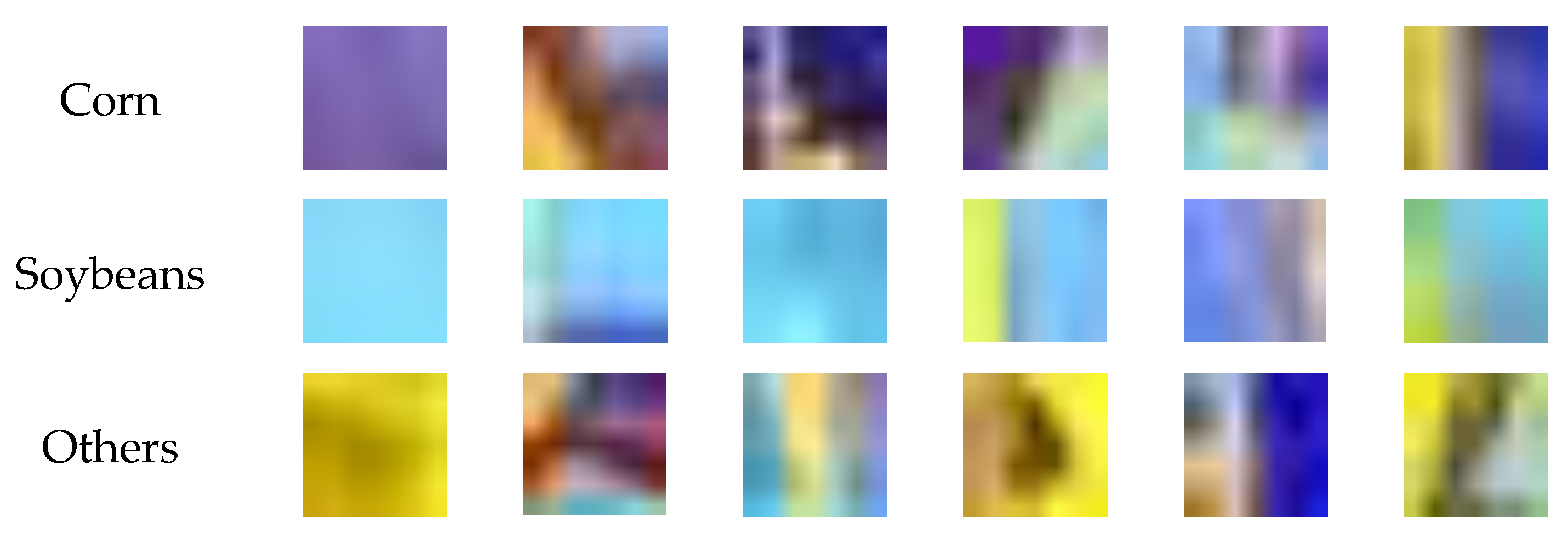
Figure 4 shows part of the training data produced from the combined data of bands 4, 3, and 2 on August 7. Our task was to classify the central pixels, and the remaining pixels in the image served as auxiliary information to help complete the classification task.

2.2. GAN Embedded CNN and LSTM

Based on the GAN model, we combined LSTM and CNN to build the final classification model to process multi-temporal and multi-band fusion data. The model performs inference and generative training at the same time during training, and only uses the discriminator during testing. This section first reviews the basic principles and model architecture of LSTM and GAN, and finally gives our method.
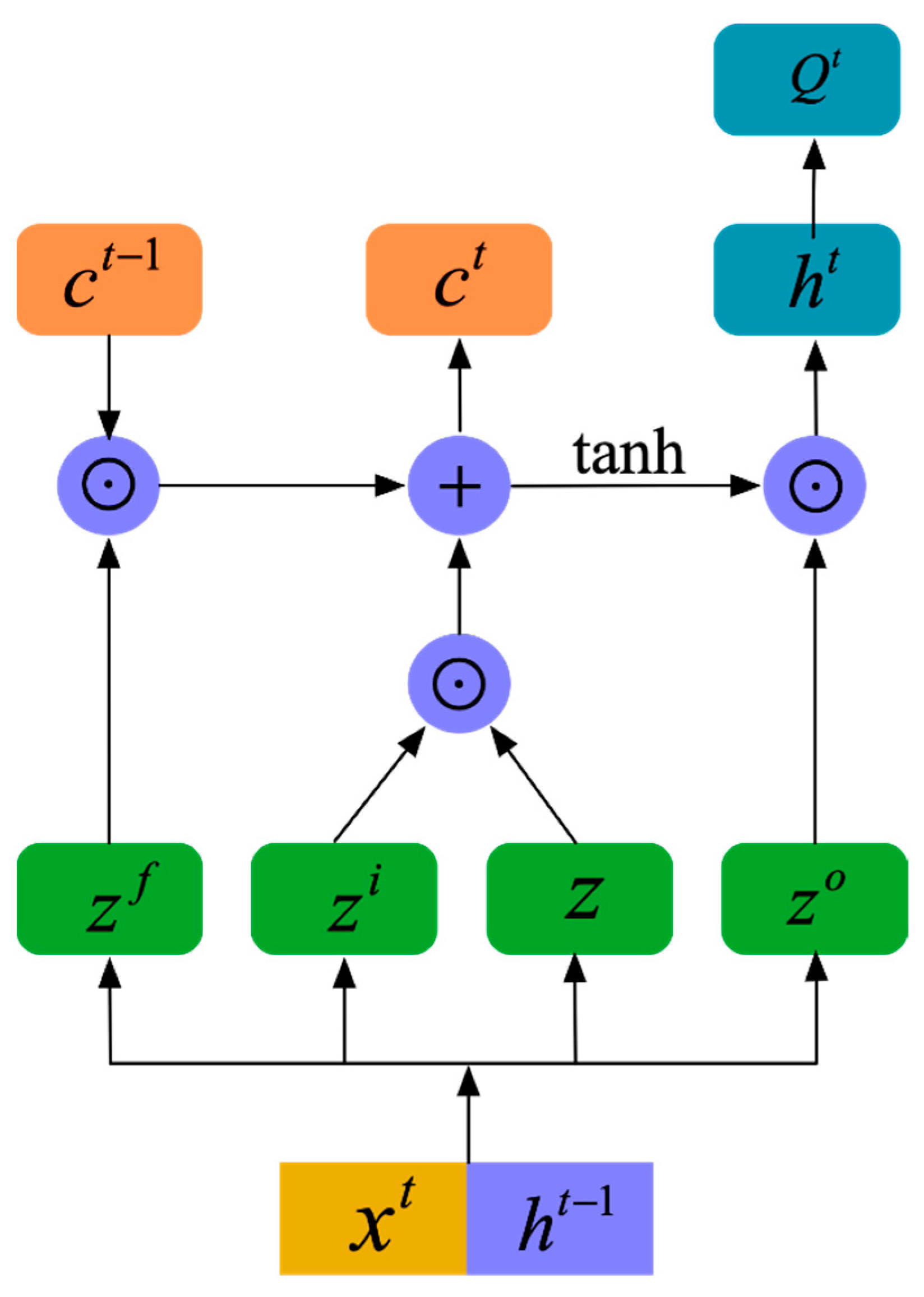
The RNN takes sequence data as input, recursively in the direction of the sequence, and all nodes are connected in a chain [13]. That is, the output of the neuron at time t-1 will be the input of the neuron at time t together with the next input. Unlike traditional neural network models, RNN can take advantage of the time dependence of data. As a variant of RNN, LSTM solves the problem of gradient disappearance and gradient explosion when using RNN to build a deeper network. Equations (1)–(7) and Figure 5 show the internal computation of the LSTM unit. stands for the Hadamard product, which multiplies the elements in two homotype matrices correspondingly. The input of LSTM is sequence variables { x 1 , , x N } , where x t is the feature vector and t is the corresponding timestamp. The γ t in the formula represents the result of the splicing between the input at time t and the h t 1 passed from the previous state.
z = tan h ( ω γ t )
z i = s i g m o i d ( ω i γ t )
z f = s i g m o i d ( ω f γ t )
z o = s i g m o i d ( ω o γ t )
c t = z f c t 1 + z i z
h t = z o tan h ( c t )
Q t = s i g m o i d ( w h t )
The LSTM unit consists of two transfer states (memory state c t and hidden state h t ) and three different gates (input gate z i , forget gate z f and output gate z o ). z i determines how much input in the current state is retained, z f determines how much information passed from the previous state needs to be forgotten, c t 1 . z o determines how much information about the current state is passed to the next state. The three gated states not only determine the information flow inside the unit but also effectively prevent the problem of gradient disappearance and explosion. z as a temporary transfer state, and the hyperbolic tangent function is used to scale the input of the current state. h t is calculated based on the newly obtained c t , and y t acts on the newly obtained h t to determine the output of the current state. The sigmoid and hyperbolic tangent functions used in the calculation process are calculated elementwise.
The adversarial generation network consists of two parts: generator G and discriminator D . The purpose of G is to learn the probability distribution of given data, and the input z is mapped to the data space G ( z ; θ g ) through a differentiable network. The essence of D is a classifier and the purpose is to correctly distinguish the data from G or the training set. G and D realize joint optimization in mutual games. Goodfellow et al. [29] proved that when the model reaches the global optimal value, the spatial distribution of G output data is equivalent to the real data distribution.
Our core idea to implement the method is to embed CNN and LSTM on the GAN model. Specifically, the discriminator is the classifier that finally completes the classification task, and CNN and LSTM are the feature extractors to extract the spatial and temporal features of the remote sensing image as the auxiliary input of the discriminator. Salimans et al. [34] once applied GAN to semi-supervised classification problems and achieved good results. Different from the general GAN, D not only needs to judge the authenticity of the image but also needs to judge the category. If the classification task requires distinguishing category k , then the output layer of D will have k + 1 neurons. Roy et al. [35] argued that it is precisely because D needs to further extract the characteristics of the generated data when making true and false judgments, leading that GAN can achieve better results than Inception Net when completing the classification task.
Salimans et al. [34] introduced a feature loss item and compares the features extracted from the real and fake images in the middle layer of the discriminator. This idea was extended by Johnson et al. [36] (perceptual loss term), which uses a certain layer of feature space of an external pre-trained network to construct the loss term. Inspired by this, we also used two pre-trained networks composed of CNN and LSTM to participate in the model construction. The difference is that the purpose of using external networks is to provide semantic information to help the discriminator judge rather than construct auxiliary loss items [37]. Specifically, we chose Inception Net [38] as the external network formed by CNN. When the input is a remote sensing image x , the extracted feature vector s ( x ) is composed of the activation value extracted by the Inception Net. We built a simple network composed of three-layer LSTM units same as Lenco et al. [39] to extract time series features t ( x ) . Remote sensing images at different times constitute different states and are input into the network in time series. The input of the discriminator is a combination of x , s ( x ) , and t ( x ) .
The overall model architecture is shown in Figure 6. The LSTM part contains two cells used to extract the temporal characteristics of the images. The input data are divided into three sequences according to time and each sequence has a dimension of 49. We set the dimension of the output feature matrix as 3 × 3 , which is convenient to be spliced with the original image as the input of the generator. It should be noted that the Inception Net model corresponding to the CNN part was trained not only on the ImageNet dataset but also on 900 agricultural images (300 each for corn, soybean, and others) by simply modifying the input layer. During the training process, we also add the reshape and convolution operation for converting the feature matrix dimension of Mixed_7c layer to 2 × 3 × 3 to concatenate with the original image. There is only one generator in our model and GAN chooses the similar generator architecture as MapGAN [40], which is mainly composed of the down-sampling layer, residual block, and up-sampling layer as shown in Figure 7. Each residual block contains two convolutional layers that do not change the dimensions of the input data. We chose patchGAN as the discriminator, and the remote sensing image is judged in patches.
The output of the discriminator is a prediction of a multi-probability distribution represented by a K + 1 dimensional logit output which comprises of K real classes and the (K + 1) class representing the fake images. We use y to represent the correct category of the discriminator corresponding to the image x . P D ( y | D ( x , s ( x ) , t ( x ) ) , y < k + 1 ) means the probability that the image x belongs to the y category output by the discriminator. The least square loss function constructed by Mao et al. [41] is used to replace the original loss function of GAN to avoid the problem of gradient disappearance and further improve the performance of the model. The loss function of the generator is:
m i n L ( G ) = 1 2 E z ~ p z ( z ) [ ( P D ( y | D ( G ( z ) , s ( G ( z ) ) , t ( G ( z ) ) ) , y < k + 1 ) 1 ) 2 ]
The loss function of the discriminator consists of a supervised loss item and an unsupervised loss item, namely m i n   L ( D ) = L s u p + L u n s u p , where:
  L s u p = E x , y ~ p d a t a ( x , y ) [ log ( P D ( y | D ( x , s ( x ) , t ( x ) ) , y < k + 1 ) ) ]
L u n s u p = 1 2 E z ~ p z ( z ) [ log ( P D ( y = k + 1 | D ( G ( z ) , s ( G ( z ) ) , t ( G ( z ) ) ) ) ) ] 1 2 E x , y ~ P d a t a ( x , y ) [ log ( 1 P D ( y = k + 1 | D ( x , s ( x ) , t ( x ) ) ) ) ]
For the meaning of each symbol, please refer to the previous part of this paper.

3. Results and Discussion

In this study, we used Landsat8 satellite imagery and CDL data to conduct experiments to explore the performance of the model in three different categories (corn, soybeans, and others). Three experiments were conducted. The first experiment explored the best multi-band combination for crop classification when the input images are in a single time term. The second experiment applied the band combination method obtained in the first group to explore the classification capability of our model when the input images are in multi time-terms. We carried out a comparison among multiple sets of models (e.g., CNN, CNN + LSTM, LSTM, GAN + CNN, SVM, SegNet, GAN + CNN + LSTM). The third experiment tested our model to perform prediction classifications in the Fayette and Pickaway County and visualize the results.

3.1. Experiment Settings

We used the Inception Net model on behalf of the CNN model, and the three LSTM units are fully connected to the SoftMax layer to represent the LSTM as the baseline model. At the same time, we combined LSTM and CNN to get a new benchmark model, in which the combination method used the feature vector extracted from the pre-trained Inception Net network Mixed_7c layer as the auxiliary input of the LSTM unit. It is worth mentioning that we set the discriminator of GAN as CNN to implement the GAN+CNN model. The initial learning rate is set to 5 × 10 4 , and the linear decay rate is 5 × 10 5 . We used the RMSProp optimizer which the square root of the sum of historical gradient controlled by the attenuation coefficient, making the learning rate of each parameter different in the training process. The proportion of the three categories in the training set and test set is approximately 1.3:1:1. The model trained a total of 200 epochs, with a batch size of 32 and a training time of about 3 min per epoch. The experiment was carried out on the workstation with one GPU of NVIDIA M40, four CPUs of Inter Xeon Platinum [email protected], and RAM: 30GiB.

3.2. Band Combination Selection

To test which band combinations can provide the most abundant and useful information of crops in multi-temporal data classification, we investigated the degree of separation of three classes in different band combinations using ENVI software [42] before conducting classification experiments. The separability is represented by the Jeffries–Matusita distance. The larger the distance value is, the better the separability is, which is more beneficial for crop classification. Based on this idea, we explored the category separability of eight different band combinations at three different dates of 2019 (July 22, August 7, and September 24). It is worth noting that we explored the combination of the three bands to balance the relationship between speed and data volume. The experimental results are shown in Table 1.
As can be seen from the table, the combination of 743, 753, and 541 has multiple Jeffries–Matusita distance values below 1.5 under three time-terms and has the worst comprehensive performance. The combination of 432 and 543 obtained a separation degree between 1.5 and 1.7, with moderate overall performance, and the 123 combination falls in between. The best-performing combinations are 564 and 562, with multiple Jeffries-Matusita distance values greater than 1.7. Among them, the separation degree of the 564 combination contains many values more than 1.8, which is the best in all the eight combinations. Interestingly, band 564 happens to be a classic combination for vegetation analysis. Therefore, the 564 band combination is more conducive to crop classification, and we will use this combination for subsequent experiments.

3.3. Acurracy Assessment of Crop Classification

To verify the ability of our method in dealing with the classification problem when the input data are time-series remote sensing images, we use Landsat8′s 564 combination band images with three time-terms on July 22, August 7, and September 24 of 2019 to form series data. To maintain the consistency, the data generated by the GAN model are also in series in this experiment. In addition, we put together seven different models for comparison. The experimental results are shown in Table 2. The order of these models in performance effects is: LSTM < CNN < CNN + LSTM < GAN + CNN < SVM < SegNet < GAN + CNN + LSTM. The experiment testing the first four models can be regarded as ablation analysis. SVM and SegNet are two state of the art models at present. Our method (GAN+CNN+LSTM) achieves the highest Kappa coefficient (0.7933) and OA accuracy (0.86). It is worth noting that all models can achieve more than 85% accuracy in the classification of corn, but this is difficult for soybeans and other categories, which range mainly from 60% to 80%. The results of the first two models show that it is not enough to use only spatial features or temporal features when completing this classification task. The result of the model CNN+LSTM proves the effectiveness of combining the spatial and temporal features. Interestingly, the result of model GAN+CNN reflects the excellent ability of GAN in completing classification tasks. We consider that this is not only due to the fact that the discriminator itself is a CNN model, but the generation training process helps the model to use more false samples in the training process. The Kappa coefficient of both SVM and SegNet is above 0.7, showing the strong competitiveness. Compared to SegNet, our model improved by 3 percentage points.

3.4. Mapping Classification Result

In order to visualize the model prediction effect more intuitively, we assigned the model prediction result to the corresponding color of the CDL image and then visualize it. Specifically, yellow represents corn, green represents soybeans, and black represents other categories. We used the seven models trained in Section 3.3 to make predictions and observations on the original images that include the training set and the test set. The results are shown in Figure 8, in which region 1 and region 2 are parts of region 3.
As we can see, the prediction results of LSTM are more confusing and the misclassification is serious, but the basic outline is shown. With the improvement of the performance of the model, the phenomena of misclassification and omission in a large area were significantly reduced, and the predict image gradually approached the ground truth image. It is worth noting that visually, our model has a visible improvement over the SVM and SegNet in the middle black area.

3.5. Model Extensibility Verification

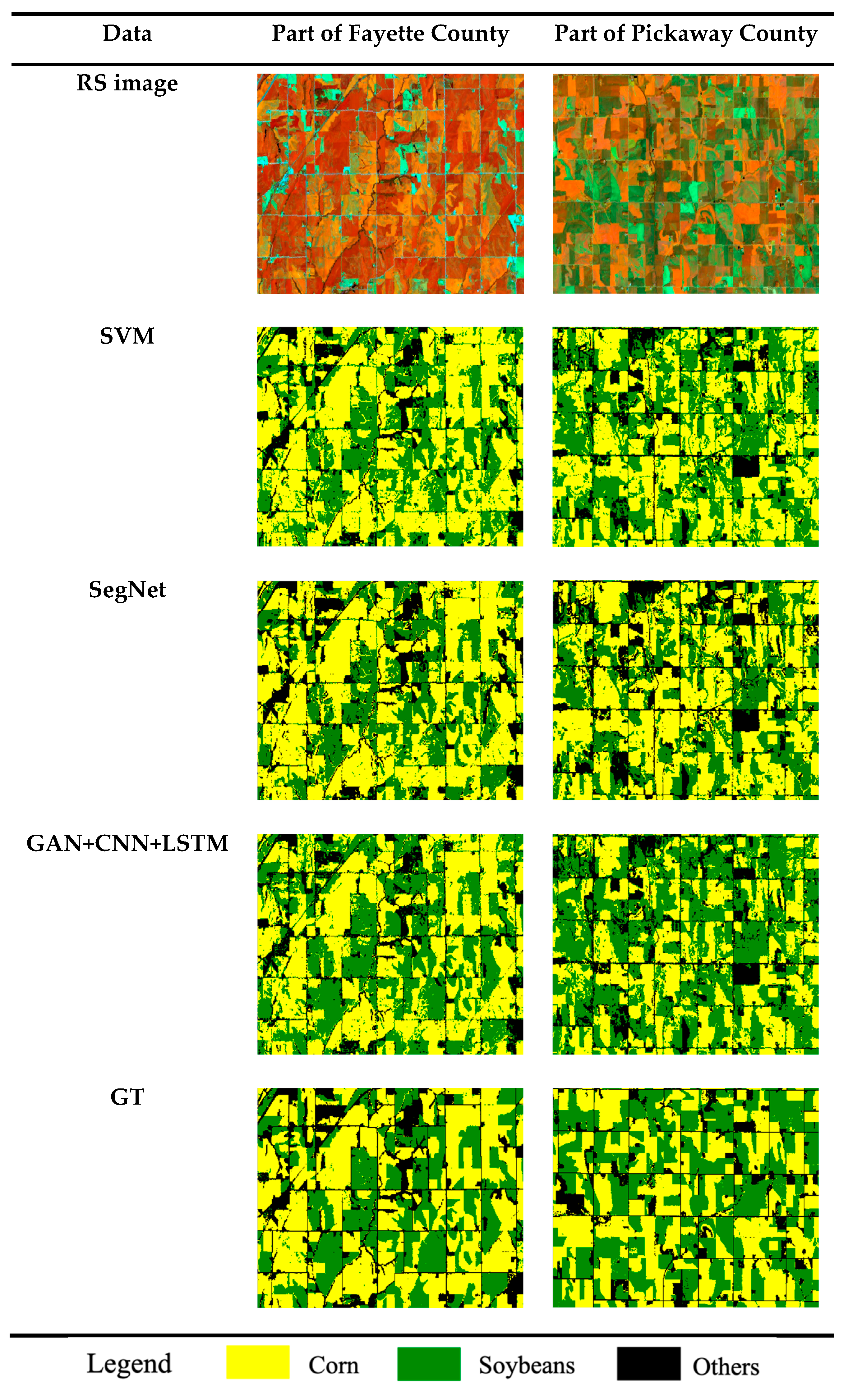
In order to verify the generalization ability of the model, we selected new test areas from Fayette and Pickaway County. The classification category remains the same, and the time-series data are still the 564 band fusion images of Landsat8 satellite of the three months of July, August, and September. In addition, we used the SVM and SegNet model for comparison considering their great performance in Section 3.4. The visualization results are shown in Figure 9. Compared with the experiment in Section 3.4, the difference between the models is more obvious in this section. The result obtained by our method has fewer noise points, more symmetrical color regions, and less misclassification. It can be seen that even for new regions, the model also has good classification capabilities. The quantitative evaluation results are shown in Table 3 and Table 4. We can see that the three models performed better in Fayette County than Pickaway County, and the relative merits were the same as the results in Section 3.3. The OA accuracy obtained by our method is 0.85 and 0.88, respectively, which does not fluctuate greatly from the 0.86 obtained in Section 3.3.

4. Conclusions

In this study, we proposed a new method that combines GAN, CNN, and LSTM models to classify crops of corn and soybeans from Landsat8 time-series images. The method is feasible on the condition that the training samples are small, and it takes advantage of spectral, spatial, and phenology features from satellite data. Experiments including band combination selection, accuracy assessment of crop classification, and model extensibility verification showed that: (1) bands of 564 of Landsat 8 are effective for crop classification; (2) our model in the study area has the highest Kappa coefficient (0.7933) and OA (86%); (3) the trained model derived from training areas in Iowa can be effectively applied to Fayette and Pickaway County, and the OA is greater than 83%. The results demonstrate that the proposed method can realize crop classification well and provide decision support for agricultural management.

Author Contributions

Conceptualization, C.Y.; methodology, J.L. and Y.S.; software, J.L.; validation, Y.S. and C.Y.; formal analysis, J.L.; investigation, C.Y.; resources, C.Y.; data curation, C.Y.; writing—original draft preparation, J.L.; writing—review and editing, Y.S. and C.Y.; visualization, Y.S.; supervision, C.Y.; project administration, C.Y. and Y.S.; funding acquisition, C.Y. All authors have read and agreed to the published version of the manuscript.

Funding

This research was funded by the Key R&D Program of Hubei Province, China under Grant No. 2020AAA004.

Institutional Review Board Statement

Not applicable

Informed Consent Statement

Not applicable

Data Availability Statement

Publicly available datasets were analyzed in this study. This data can be found here: [https://pan.baidu.com/s/1rCKX3Q6o5OLu7OBH0XtEHA with secret xtj2].

Acknowledgments

The authors would like to thank the reviewers and associate editor for their valuable comments and suggestions to improve the quality of the paper.

Conflicts of Interest

The authors declare no conflict of interest.

References

  1. Zhai, Y.; Wang, N.; Zhang, L.; Hao, L.; Hao, C. Automatic crop classification in northeastern China by improved nonlinear dimensionality reduction for satellite image time series. Remote Sens. 2020, 12, 2726. [Google Scholar] [CrossRef]
  2. Bin, W.A.N.G.; Doglin, F.A.N. Research progress of deep learning in classification and recognition of remote sensing images. Bull. Surv. Mapp. 2019, 2, 99–102. [Google Scholar]
  3. Reed, B.C.; Brown, J.F.; VanderZee, D.; Loveland, T.R.; Merchant, J.W.; Ohlen, D.O. Measuring phenological variability from satellite imagery. J. Veg. Sci. 1994, 5, 703–714. [Google Scholar] [CrossRef]
  4. Zhang, J. Multi-source remote sensing data fusion: Status and trends. Int. J. Image Data Fusion 2010, 1, 5–24. [Google Scholar] [CrossRef] [Green Version]
  5. Wulder, M.A.; Loveland, T.R.; Roy, D.P.; Crawford, C.J.; Masek, J.G.; Woodcock, C.E.; Allen, R.G.; Anderson, M.C.; Belward, A.S.; Cohen, W.B.; et al. Current status of Landsat program, science, and applications. Remote Sens. Environ. 2019, 225, 127–147. [Google Scholar] [CrossRef]
  6. Kotsiantis, S.B.; Zaharakis, I.; Pintelas, P. Supervised machine learning: A review of classification techniques. Emerg. Artif. Intell. Appl. Comput. Eng. 2007, 160, 3–24. [Google Scholar]
  7. Mohd, H.I.; Pakhriazad, H.Z.; Shahrin, M.F. Evaluating supervised and unsupervised techniques for land cover mapping using remote sensing data. Geogr. Malays. J. Soc. Space 2009, 5, 1–10. [Google Scholar]
  8. Bazi, Y.; Melgani, F. Toward an optimal SVM classification system for hyperspectral remote sensing images. IEEE Trans. Geosci. Remote. Sens. 2006, 44, 3374–3385. [Google Scholar] [CrossRef]
  9. Hui, C.; Huicheng, L. An improved BP neural network algorithm and its application. Comput. Simul. 2007, 24, 75–77. [Google Scholar]
  10. Liu, B.; Du, S.; Du, S.; Zhang, X. Incorporating deep features into GEOBIA paradigm for remote sensing imagery classification: A patch-based approach. Remote Sens. 2020, 12, 3007. [Google Scholar] [CrossRef]
  11. Gaoming, X.; Kai, H. The application of Tsinghua Sunway EPS software in the census of geographical conditions. Surv. Spat. Geogr. Inf. 2014, 37, 198–200. [Google Scholar]
  12. Ma, L.; Liu, Y.; Zhang, X.; Ye, Y.; Yin, G.; Johnson, B.A. Deep learning in remote sensing applications: A meta-analysis and review. ISPRS J. Photogramm. Remote Sens. 2019, 152, 166–177. [Google Scholar] [CrossRef]
  13. Chen, Y.; Zhao, X.; Jia, X. Spectral–spatial classification of hyperspectral data based on deep belief network. IEEE J. Sel. Top. Appl. Earth Obs. Remote Sens. 2015, 8, 2381–2392. [Google Scholar] [CrossRef]
  14. Krizhevsky, A.; Sutskever, I.; Hinton, G.E. Imagenet classification with deep convolutional neural networks. Ina. Neural Inf. Process. Syst. 2012, 60, 1097–1105. [Google Scholar] [CrossRef]
  15. Masci, J.; Meier, U.; Cireşan, D.; Schmidhuber, J. Stacked convolutional auto-encoders for hierarchical feature extraction. In International Conference on Artificial Neural Networks, Proceedings of the 21st International Conference on Artificial Neural Networks, Espoo, Finland, 14–17 June 2011; Springer: Berlin/Heidelberg, Germany, 2011; pp. 52–59. [Google Scholar]
  16. Zhang, D.; Wang, D. Relation classification via recurrent neural network. arXiv 2015, arXiv:1508.01006. [Google Scholar]
  17. Kaiyu, W.; Huihua, Y. Hyperspectral remote sensing image classification based on landmark spatial information. Vedio Eng. 2017, 41, 69–73. [Google Scholar]
  18. Cao, X.; Yao, J.; Xu, Z.; Meng, D. Hyperspectral Image Classification With Convolutional Neural Network and Active Learning. IEEE T. Geosci. Remote 2020, 58, 4604–4616. [Google Scholar] [CrossRef]
  19. Hsieh, T.-H.; Kiang, J.-F. Comparison of CNN algorithms on hyperspectral image classification in agricultural lands. Sensors 2020, 20, 1734. [Google Scholar] [CrossRef] [Green Version]
  20. Liang, P.; Shi, W.; Zhang, X. Remote sensing image classification based on stacked denoising autoencoder. Remote Sens. 2018, 10, 16. [Google Scholar] [CrossRef] [Green Version]
  21. Baatz, M.; Schäpe, A. Multiresolution Segmentation: An Optimization Approach for High Quality Multi-Scale Image Segmentation. Available online: http://www.agit.at/papers/2000/baatz_FP_12.Pdf (accessed on 25 December 2020).
  22. Ebrahimi, J.; Dou, D. Chain based RNN for relation classification. In Proceedings of the 2015 Conference of the North American Chapter of the Association for Computational Linguistics: Human Language Technologies, Denver, CO, USA, 31 May–5 June 2015; pp. 1244–1249. [Google Scholar]
  23. Graves, A.; Mohamed, A.R.; Hinton, G. Speech recognition with deep recurrent neural networks. In Proceedings of the Advances in 2013 IEEE International Conference on Acoustics, Speech and Signal Processing, Vancouver, BC, Canada, 26–30 May 2013; pp. 6645–6649. [Google Scholar]
  24. Linzen, T.; Dupoux, E.; Goldberg, Y. Assessing the ability of LSTMs to learn syntax-sensitive dependencies. Trans. ACL 2016, 4, 521–535. [Google Scholar] [CrossRef]
  25. Greff, K.; Srivastava, R.K.; Koutník, J.; Steunebrink, B.R.; Schmidhuber, J. LSTM: A Search Space Odyssey. arXiv 2015, arXiv:1502.04390. Available online: https://arxiv.org/abs/1502.04390v1 (accessed on 12 February 2015). [CrossRef] [PubMed] [Green Version]
  26. Ndikumana, E.; Ho Tong Minh, D.; Baghdadi, N.; Courault, D.; Hossard, L. Deep recurrent neural network for agricultural classification using multitemporal SAR Sentinel-1 for Camargue, France. Remote Sens. 2018, 10, 1217. [Google Scholar] [CrossRef] [Green Version]
  27. Sun, Z.H.; Di, L.P.; Fang, H. Using long short-term memory recurrent neural network in land cover classification on Landsat and Cropland data layer time series. Int. J. Remote Sens. 2019, 40, 593–614. [Google Scholar] [CrossRef]
  28. Zhang, G.; Rui, X.; Poslad, S.; Song, X.; Fan, Y.; Ma, Z. Large-Scale, Fine-Grained, Spatial, and Temporal. Sensors 2019, 19, 2156. [Google Scholar] [CrossRef] [Green Version]
  29. Goodfellow, I.; Pouget-Abadie, J.; Mirza, M.; Xu, B.; Warde-Farley, D.; Ozair, S.; Courville, A.; Bengio, Y. Generative adversarial nets. In Proceedings of the Advances in Neural Information Processing Systems (NIPS), Montreal, QC, Canada, 8–13 December 2014; pp. 2672–2680. [Google Scholar]
  30. Zeng, J.; Wu, Y.; Liu, J.G.; Wang, L.; Hu, J. Learning and inference on generative adversarial quantum circuits. Phys. Rev. A 2019, 99, 052306. [Google Scholar] [CrossRef] [Green Version]
  31. USDA National Agricultural Statistics Service Cropland Data Layer. Published Crop-Specific Data Layer. Verified USDA-NASS, Washington, DC. 2019. Available online: https://nassgeodata.gmu.edu/CropScape/ (accessed on 10 May 2020).
  32. Johnson, D.M. Using the Landsat archive to map crop cover history across the United States. Remote Sens. Environ. 2019, 232, 111286. [Google Scholar] [CrossRef]
  33. Gao, F.; Anderson, M.C.; Zhang, X. Toward mapping crop progress at field scales through fusion of Landsat and MODIS imagery. Remote Sens. Environ. 2017, 188, 9–25. [Google Scholar] [CrossRef] [Green Version]
  34. Salimans, T.; Goodfellow, I.; Zaremba, W.; Cheung, V.; Radford, A.; Chen, X. Improved techniques for training gans. In Proceedings of the Advances in Neural Information Processing Systems (NIPS), Barcelona, Spain, 4–9 December 2016; pp. 2234–2242. [Google Scholar]
  35. Roy, S.; Sangineto, E.; Sebe, N.; Demir, B. Semantic-fusion gans for semi-supervised satellite image classification. In Proceedings of the 25th IEEE International Conference on Image Processing (ICIP), Athens, Greece, 7–10 October 2018; pp. 684–688. [Google Scholar]
  36. Johnson, J.; Alahi, A.; Fei-Fei, L. Perceptual losses for real-time style transfer and super-resolution. In Proceedings of the European Conference on Computer Vision, Amsterdam, The Netherlands, 8–16 October 2016; pp. 694–711. [Google Scholar]
  37. Bazi, Y.; Al Rahhal, M.M.; Alhichri, H.; Alajlan, N. Simple yet effective fine-tuning of deep CNNs using an auxiliary classification loss for remote sensing scene classification. Remote Sens. 2019, 11, 2908. [Google Scholar] [CrossRef] [Green Version]
  38. Szegedy, C.; Vanhoucke, V.; Ioffe, S.; Shlens, J.; Wojna, Z. Rethinking the inception architecture for computer vision. In Proceedings of the IEEE conference on computer vision and pattern recognition, Las Vegas, NV, USA, 26 June–1 July 2016; pp. 2818–2826. [Google Scholar]
  39. Ienco, D.; Gaetano, R.; Dupaquier, C.; Maurel, P. Land cover classification via multitemporal spatial data by deep recurrent neural networks. IEEE Geosci Remote Sens. Lett. 2017, 1685–1689. [Google Scholar] [CrossRef] [Green Version]
  40. Li, J.; Chen, Z.; Zhao, X.; Shao, L. MapGAN: An intelligent generation model for network tile maps. Sensors 2020, 20, 3119. [Google Scholar] [CrossRef]
  41. Mao, X.D.; Li, Q.; Xie, H.R.; Raymond, Y.K.; Wang, Z.; Smalley, S.P. Least Squares Generative Adversarial Networks. In Proceedings of the IEEE International Conference on Computer Vision (ICCV), Venice, Italy, 22–29 October 2017; pp. 2794–2802. [Google Scholar]
  42. Liu, X.K.; Zhai, H.; Shen, Y.L.; Lou, B.K.; Jiang, C.M.; Li, T.Q.; Hussain, S.; Shen, G.L. Large-scale crop mapping from multisource remote sensing images in google earth engine. IEEE J. Sel. Top. Appl. Earth Obs. Remote Sens. 2020, 13, 414–427. [Google Scholar] [CrossRef]
Figure 1. Study areas concentrated in Iowa, Ohio, and Pennsylvania States.
Remotesensing 13 00065 g001
Figure 2. Part of the training data produced: (a) 432 band fusion image; (b) 652 band fusion map; (c) 564 band fusion map; (d) corresponding CDL data. (ac) are obtained by Landsat 8 satellite on 7 August 2019.
Remotesensing 13 00065 g002
Figure 3. Example of making a training sample pair. The fixed-size window is slidingly cut on the input remote sensing image, and the crop type label corresponding to each remote sensing image is the crop with the center point at the corresponding position of the CDL image.
Remotesensing 13 00065 g003
Figure 4. Part of the training examples.
Remotesensing 13 00065 g004
Figure 5. The internal structure of the long- and short-term memory neural network (LSTM) unit.
Remotesensing 13 00065 g005
Figure 6. Overall model architecture.
Remotesensing 13 00065 g006
Figure 7. The generator architecture.
Remotesensing 13 00065 g007
Figure 8. Visualization of the results of the model trained in the second experiment on the original image.
Remotesensing 13 00065 g008aRemotesensing 13 00065 g008b
Figure 9. Visualization of the prediction results of the model in Fayette County and Pickaway County.
Remotesensing 13 00065 g009
Table 1. Jeffries–Matusita distance of the three categories in different band combinations at different times.
NO.Band CombinationCrop22 July 20197 August 201924 September 2019
TypeCorn Soybeans OthersCorn Soybeans OthersCorn Soybeans Others
15, 6, 4Corn1.001.861.931.001.731.871.001.791.82
Soybeans1.861.001.761.731.001.741.791.001.85
Others1.931.761.001.871.741.001.821.851.00
25, 6, 2Corn1.001.611.791.001.771.831.001.621.84
Soybeans1.611.001.681.771.001.811.621.001.59
Others1.791.681.001.831.811.001.841.591.00
34, 3, 2Corn1.001.501.621.001.661.721.001.571.54
Soybeans1.501.001.571.661.001.681.571.001.71
Others1.621.571.001.721.681.001.541.711.00
4.5, 4, 3Corn1.001.761.681.001.671.831.001.551.62
Soybeans1.761.001.531.671.001.571.551.001.64
Others1.681.531.001.831.571.001.621.641.00
51, 2, 3Corn1.001.581.651.001.751.491.001.601.67
Soybeans1.581.001.471.751.001.561.601.001.53
Others1.651.471.001.491.561.001.671.531.00
65, 4, 1Corn1.001.211.831.001.421.561.001.511.68
Soybeans1.211.001.471.421.001.631.511.001.61
Others1.831.471.001.561.631.001.681.611.00
77, 4, 3Corn1.001.601.821.001.471.661.001.461.73
Soybeans1.601.001.391.471.001.281.461.001.51
Others1.821.391.001.661.281.001.731.511.00
87, 5, 4Corn1.001.251.561.001.591.571.001.371.64
Soybeans1.251.001.771.591.001.681.371.001.72
Others1.561.771.001.571.681.001.641.721.00
Table 2. Classification accuracy of seven different models on multi-temporal and multi-band data sets.
NO.ModelCropConfusion Matrix (%)Kappa CoefficientOA
TypeCorn Soybeans Others
1LSTMCorn92.360.637.010.33690.54
Soybeans62.6732.534.80
Others20.1844.1235.70
2CNNCorn89.542.517.940.46340.64
Soybeans26.2168.195.60
Others43.4620.136.44
3CNN+LSTMCorn86.9411.411.650.51400.68
Soybeans4.0187.398.60
Others4.6878.0417.28
4GAN+CNNCorn97.280.382.340.64980.77
Soybeans38.7253.717.57
Others12.237.6380.14
5SVMCorn92.657.130.220.72220.81
Soybeans7.2787.894.84
Others4.6530.4164.94
6SegNetCorn96.211.462.330.75780.83
Soybeans12.5970.028.39
Others12.826.9680.22
7GAN+CNN+LSTMCorn97.551.131.320.79330.86
Soybeans12.8480.216.95
Others10.3311.2478.43
Table 3. Quantitative evaluation of the model’s prediction results in Fayette County.
NO.ModelCropConfusion Matrix (%)Kappa CoefficientOA
TypeCorn Soybeans Others
1SVMCorn88.537.144.330.65410.75
Soybeans17.371.8310.87
Others14.5112.2973.2
2SegNetCorn92.174.253.580.71860.81
Soybeans16.572.1411.36
Others10.3919.2770.34
3GAN+CNN+LSTMCorn90.316.722.970.76350.85
Soybeans5.3781.4213.21
Others9.3413.876.86
Table 4. Quantitative evaluation of the model’s prediction results in Pickaway County.
NO.ModelCropConfusion Matrix (%)Kappa CoefficientOA
TypeCorn Soybeans Others
1SVMCorn91.475.123.410.74260.83
Soybeans13.8774.6611.47
Others7.9121.7271.37
2SegNetCorn93.953.082.970.76510.87
Soybeans15.9177.826.27
Others11.9010.8977.21
3GAN+CNN+LSTMCorn90.937.621.450.77010.88
Soybeans3.6087.219.19
Others3.0423.5273.44
Publisher’s Note: MDPI stays neutral with regard to jurisdictional claims in published maps and institutional affiliations.