
Rotation Invariance Regularization for Remote Sensing Image Scene Classification with Convolutional Neural Networks


Abstract
1. Introduction
2. Related Work
2.1. DCNN-Based Scene Classification
2.2. Rotation Invariance Features
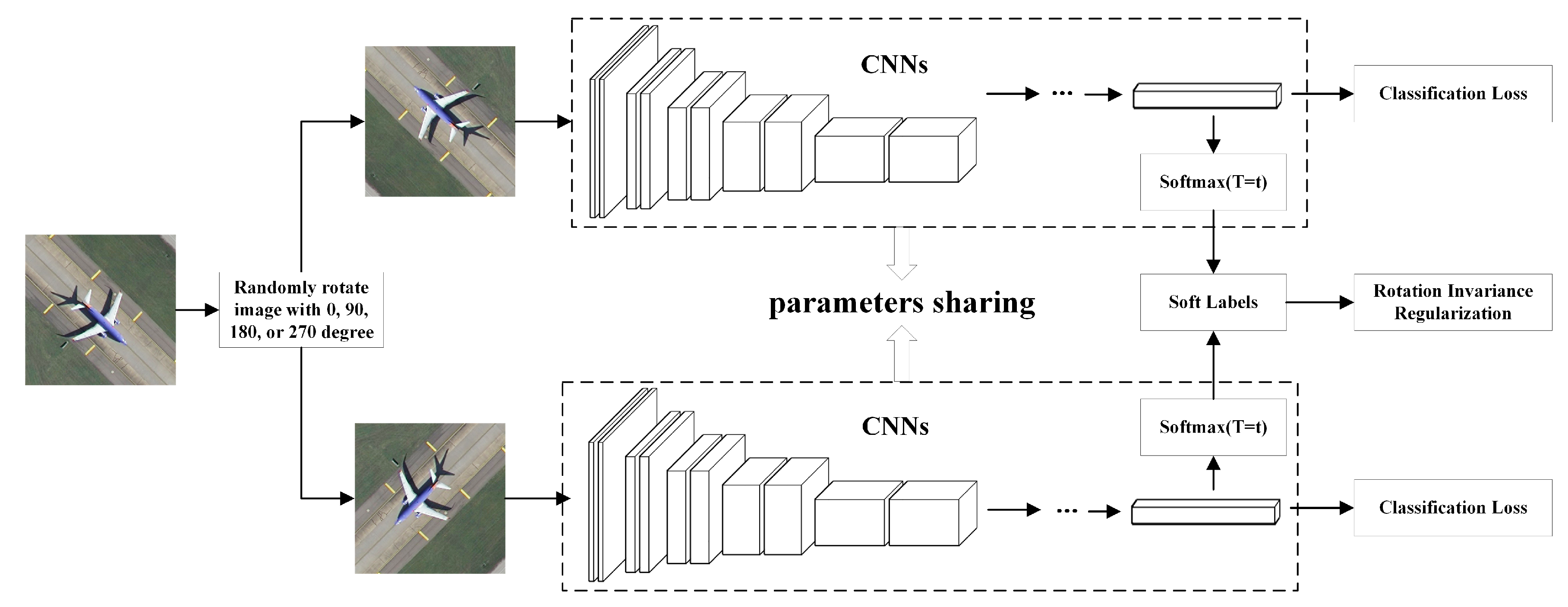
3. Proposed Method
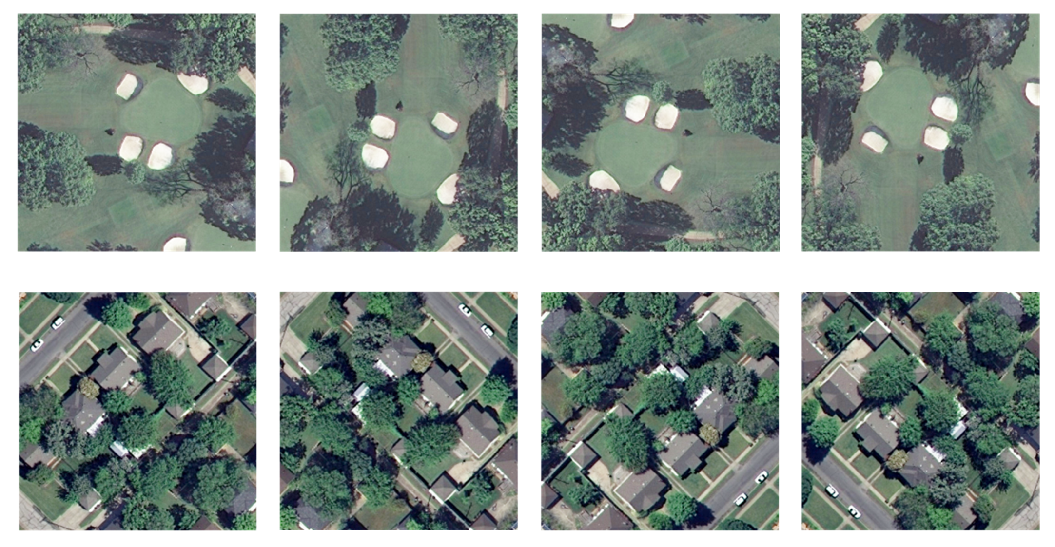
3.1. Data Augmentation
3.2. Rotation Invariance Regularization
4. Experiments
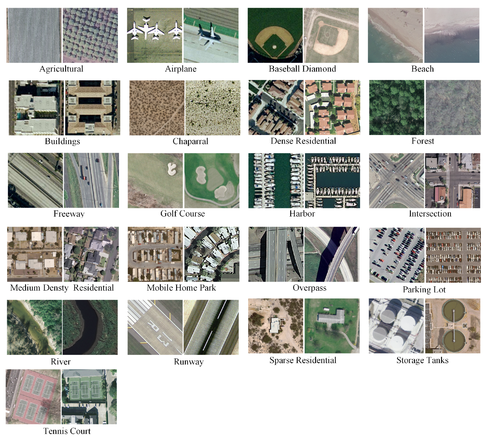
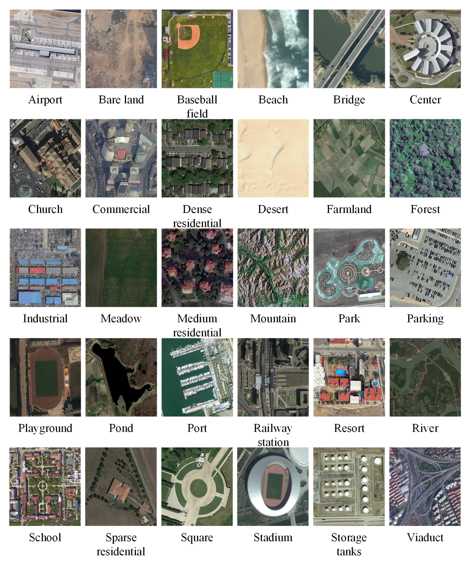
4.1. Data Sets
4.2. Experimental Setup
4.3. Implementation
5. Results and Discussion
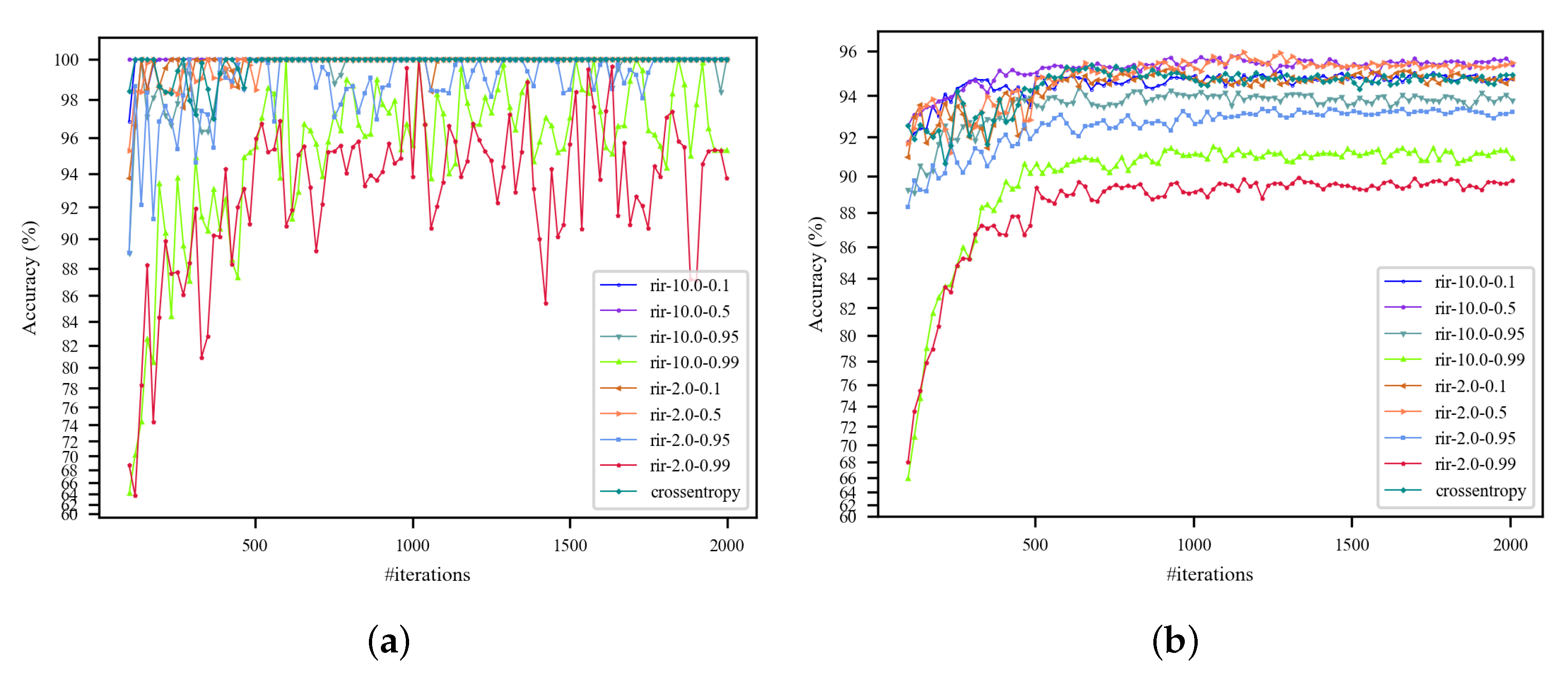
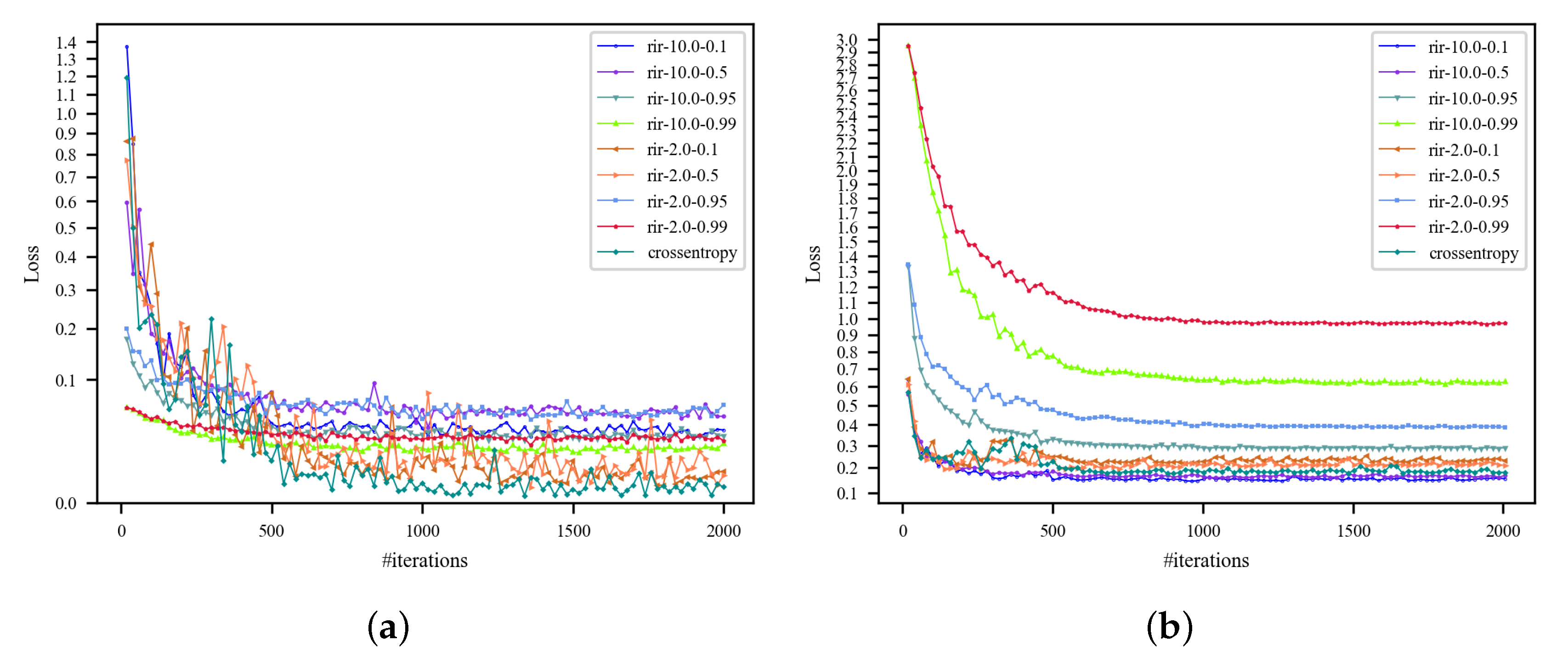
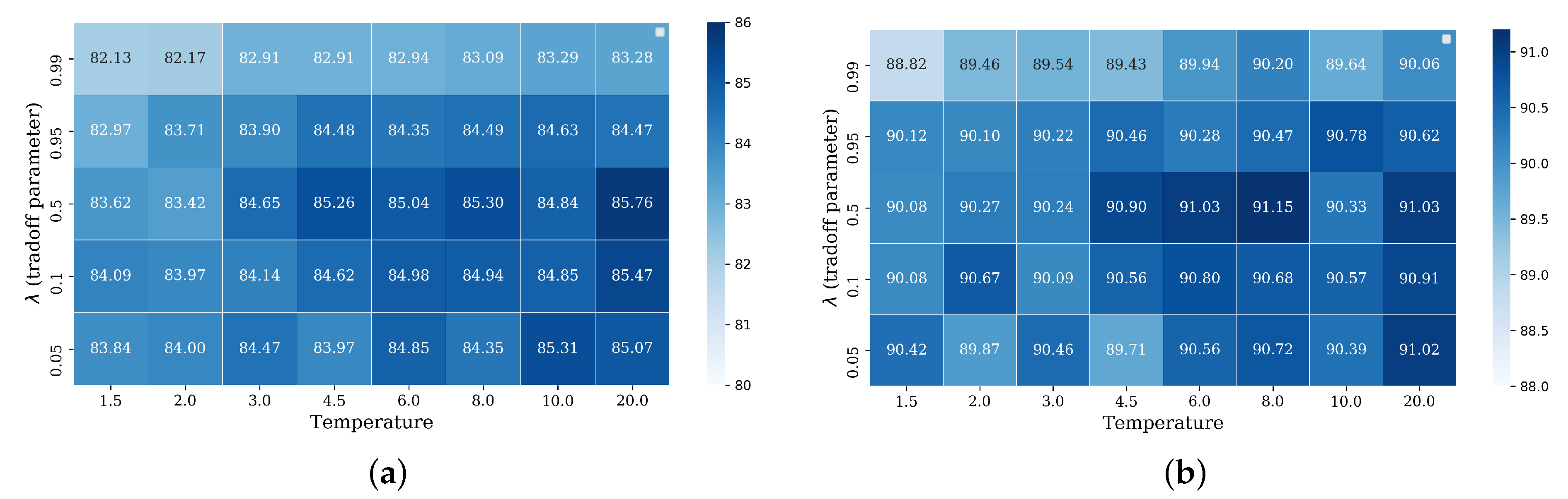
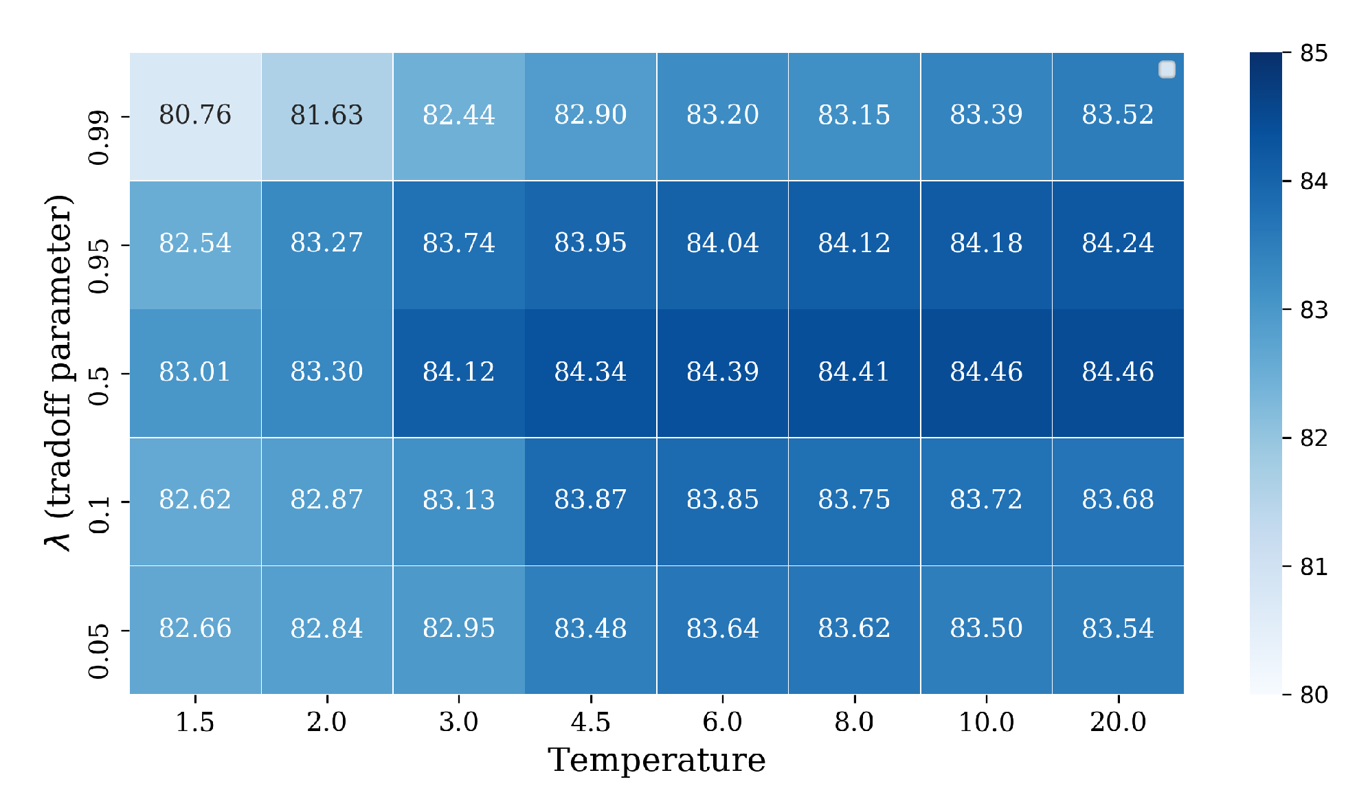
5.1. Tradeoff of Temperature and Tuning Parameters
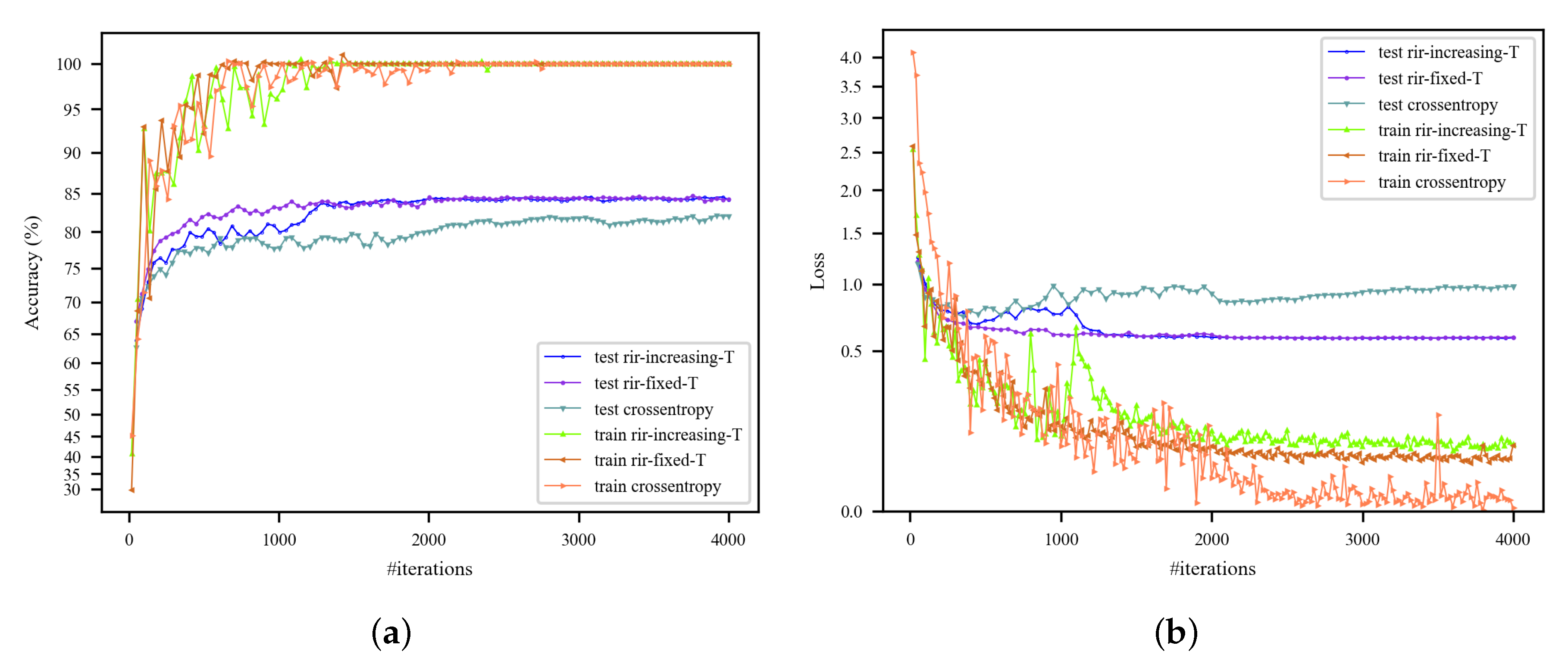
5.2. Effect of Increasing Temperature Strategy
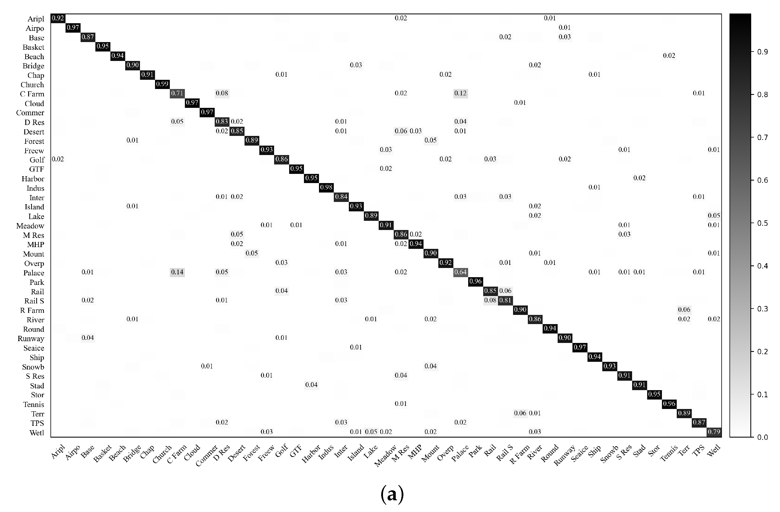
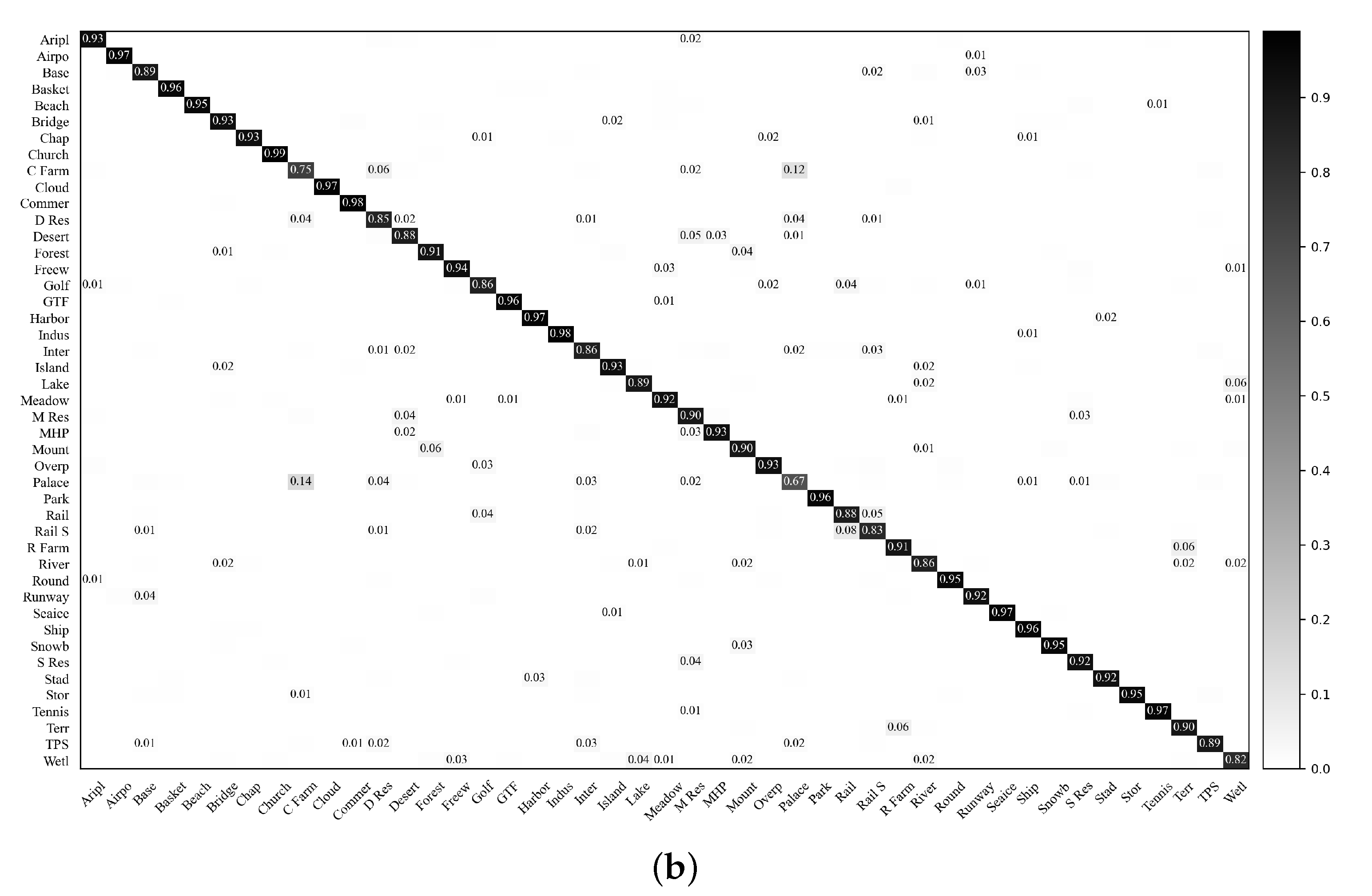
5.3. Validation on the AID Data Set
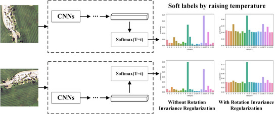
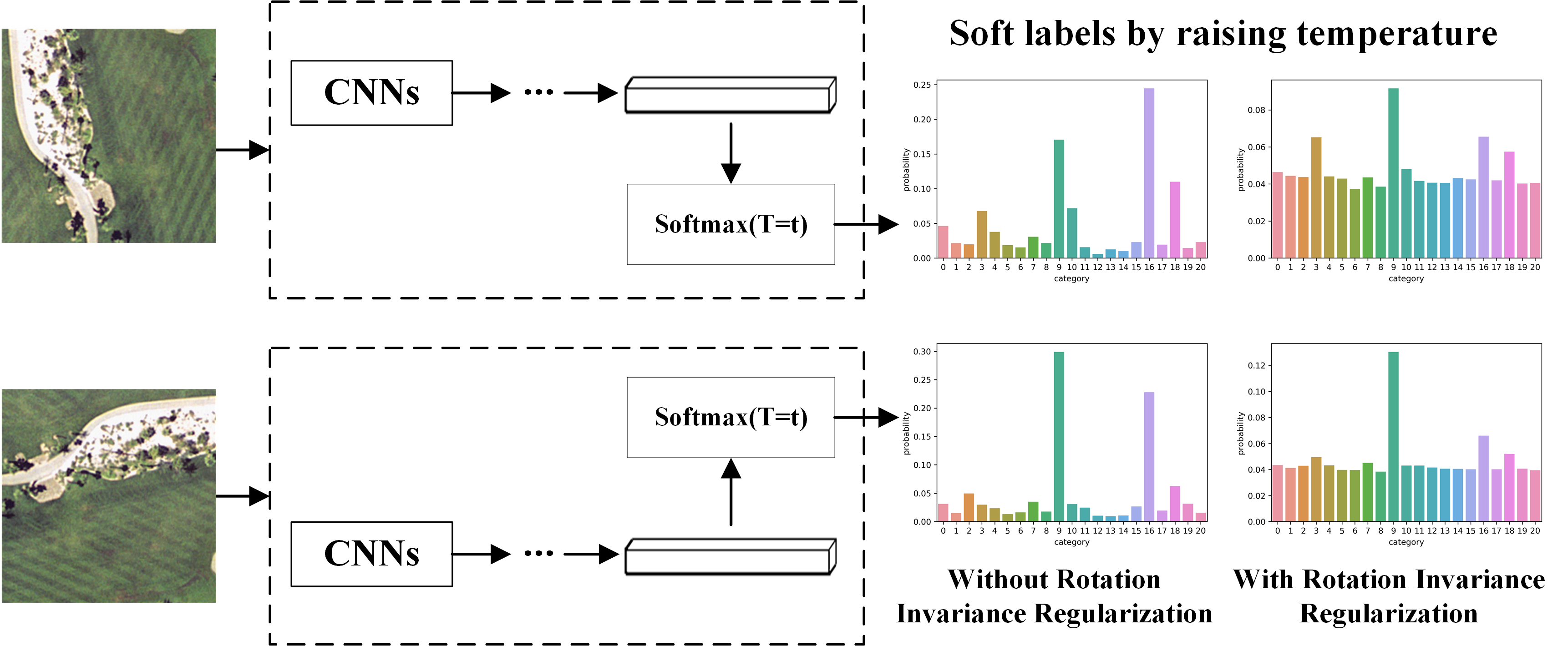
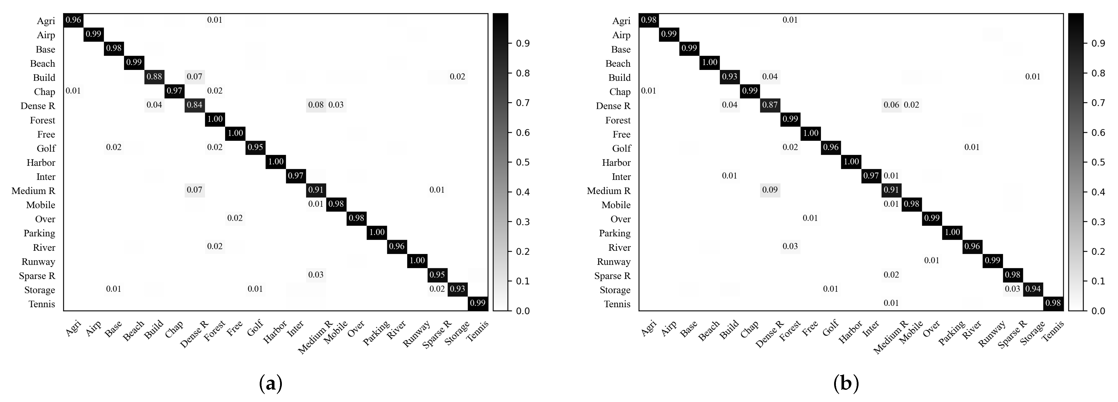
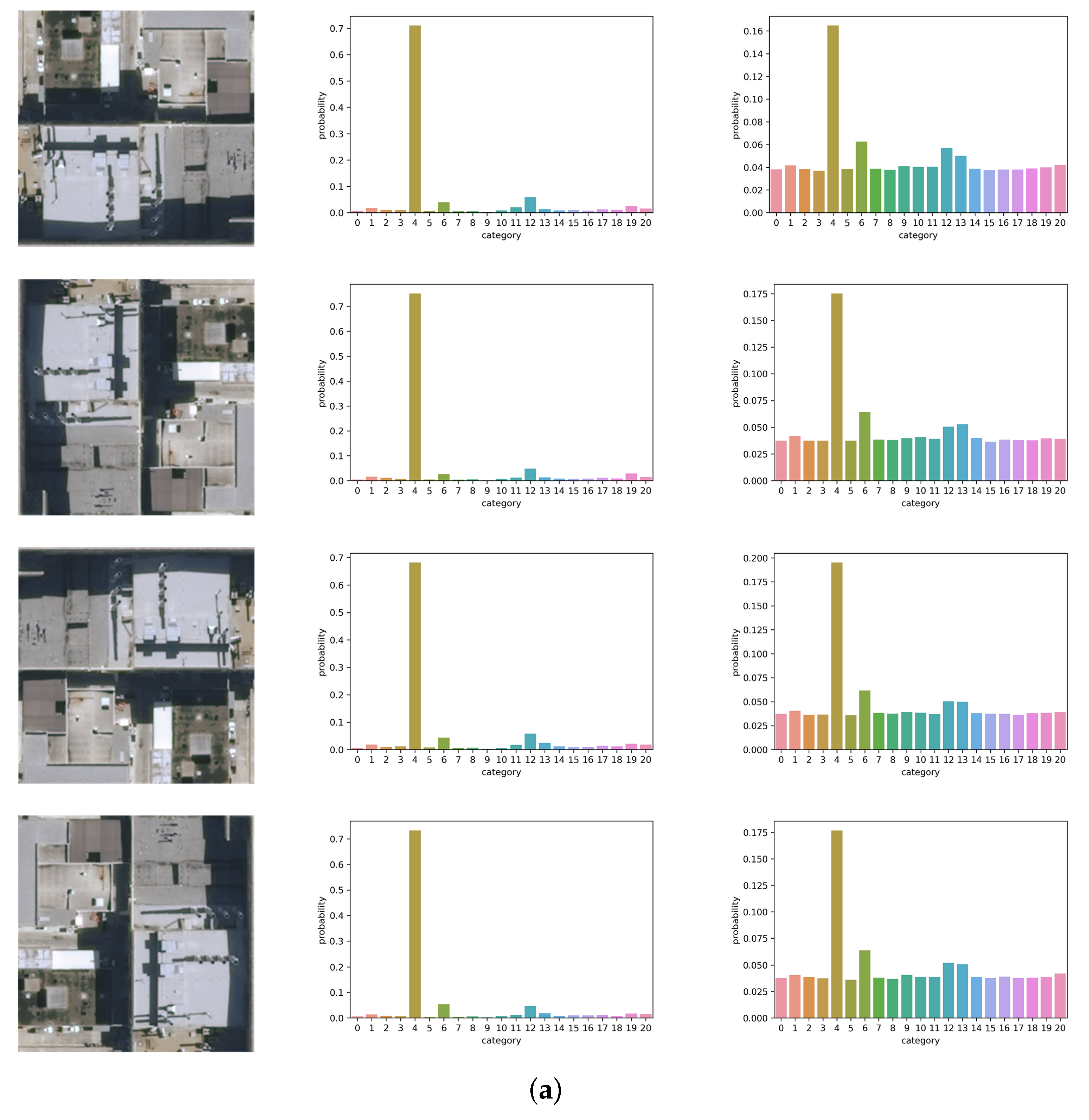
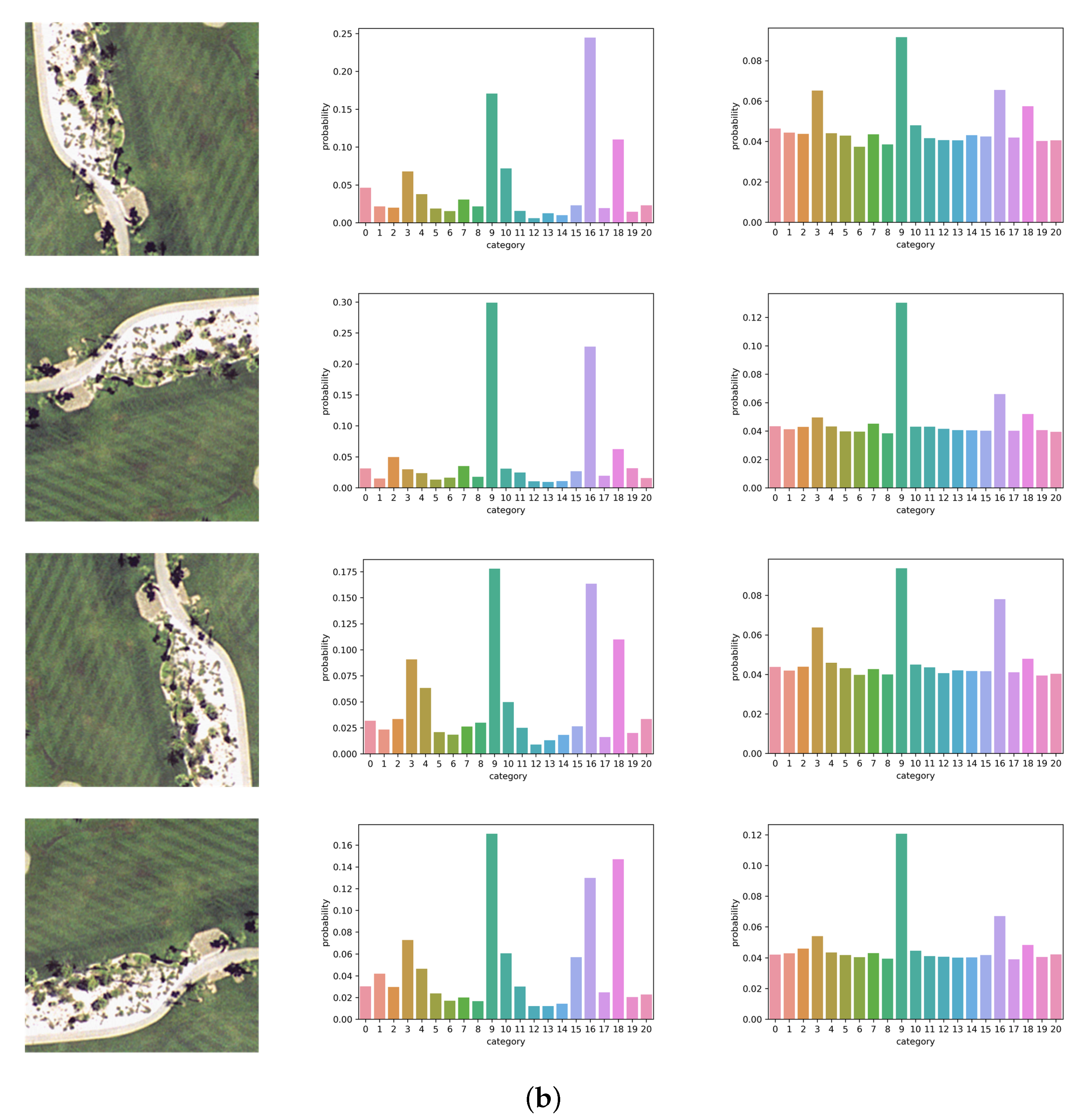
5.4. Visualization of the Softmax Outputs
6. Conclusions
Author Contributions
Funding
Institutional Review Board Statement
Informed Consent Statement
Data Availability Statement
Acknowledgments
Conflicts of Interest
References
- Cheng, G.; Han, J.; Lu, X. Remote sensing image scene classification: Benchmark and state of the art. Proc. IEEE 2017, 105, 1865–1883. [Google Scholar] [CrossRef]
- Yang, Y.; Newsam, S. Geographic image retrieval using local invariant features. IEEE Trans. Geosci. Remote Sens. 2013, 51, 818–832. [Google Scholar] [CrossRef]
- Martha, T.R.; Kerle, N.; van Westen, C.J.; Jetten, V.; Kumar, K.V. Segment optimization and data-driven thresholding for knowledge-based landslide detection by object-based image analysis. IEEE Trans. Geosci. Remote Sens. 2011, 49, 4928–4943. [Google Scholar] [CrossRef]
- Qi, K.; Wu, H.; Shen, C.; Gong, J. Land-use scene classification in high-resolution remote sensing images using improved correlatons. IEEE Geosci. Remote Sens. Lett. 2015, 12, 2403–2407. [Google Scholar]
- Du, Z.; Li, X.; Lu, X. Local structure learning in high resolution remote sensing image retrieval. Neurocomputing 2016, 207, 813–822. [Google Scholar] [CrossRef]
- Chen, Z.; Zhang, T.; Ouyang, C. End-to-end airplane detection using transfer learning in remote sensing images. Remote Sens. 2018, 10, 139. [Google Scholar] [CrossRef]
- Oquab, M.; Bottou, L.; Laptev, I.; Sivic, J. Learning and transferring mid-level image representations using convolutional neural networks. In Proceedings of the IEEE Conference on Computer Vision and Pattern Recognition, Columbus, OH, USA, 23–28 June 2014; pp. 1717–1724. [Google Scholar]
- Penatti, O.A.; Nogueira, K.; Dos Santos, J.A. Do deep features generalize from everyday objects to remote sensing and aerial scenes domains? In Proceedings of the IEEE Conference on Computer Vision and Pattern Recognition, Boston, MA, USA, 7–12 June 2015; pp. 44–51. [Google Scholar]
- Hu, F.; Xia, G.S.; Hu, J.; Zhang, L. Transferring deep convolutional neural networks for the scene classification of high-resolution remote sensing imagery. Remote Sens. 2015, 7, 14680–14707. [Google Scholar] [CrossRef]
- Romero, A.; Gatta, C.; Camps-Valls, G. Unsupervised deep feature extraction for remote sensing image classification. IEEE Trans. Geosci. Remote Sens. 2016, 54, 1349–1362. [Google Scholar] [CrossRef]
- Cheng, G.; Yang, C.; Yao, X.; Guo, L.; Han, J. When deep learning meets metric learning: Remote sensing image scene classification via learning discriminative CNNs. IEEE Trans. Geosci. Remote Sens. 2018, 56, 2811–2821. [Google Scholar] [CrossRef]
- Pires de Lima, R.; Marfurt, K. Convolutional neural network for remote-sensing scene classification: Transfer learning analysis. Remote Sens. 2020, 12, 86. [Google Scholar] [CrossRef]
- Li, E.; Xia, J.; Du, P.; Lin, C.; Samat, A. Integrating multilayer features of convolutional neural networks for remote sensing scene classification. IEEE Trans. Geosci. Remote Sens. 2017, 55, 5653–5665. [Google Scholar] [CrossRef]
- Qi, K.; Guan, Q.; Yang, C.; Peng, F.; Shen, S.; Wu, H. Concentric Circle Pooling in Deep Convolutional Networks for Remote Sensing Scene Classification. Remote Sens. 2018, 10, 934. [Google Scholar] [CrossRef]
- Xie, J.; He, N.; Fang, L.; Plaza, A. Scale-free convolutional neural network for remote sensing scene classification. IEEE Trans. Geosci. Remote Sens. 2019, 57, 6916–6928. [Google Scholar] [CrossRef]
- Zhang, J.; Liu, J.; Pan, B.; Shi, Z. Domain Adaptation Based on Correlation Subspace Dynamic Distribution Alignment for Remote Sensing Image Scene Classification. IEEE Trans. Geosci. Remote. Sens. 2020, 58, 7920–7930. [Google Scholar] [CrossRef]
- Swain, M.J.; Ballard, D.H. Color indexing. Int. J. Comput. Vis. 1991, 7, 11–32. [Google Scholar] [CrossRef]
- Lowe, D.G. Distinctive Image Features from Scale-Invariant Keypoints. Int. J. Comput. Vis. 2004, 60, 91–110. [Google Scholar] [CrossRef]
- Dalal, N.; Triggs, B. Histograms of oriented gradients for human detection. In Proceedings of the 2005 IEEE Computer Society Conference on Computer Vision and Pattern Recognition, San Diego, CA, USA, 20–25 June 2005; IEEE Computer Society: Washington, DC, USA, 2005; Volume 1, pp. 886–893. [Google Scholar]
- Oliva, A.; Torralba, A. Modeling the shape of the scene: A holistic representation of the spatial envelope. Int. J. Comput. Vis. 2001, 42, 145–175. [Google Scholar] [CrossRef]
- Krizhevsky, A.; Sutskever, I.; Hinton, G.E. Imagenet classification with deep convolutional neural networks. In Proceedings of the 25th International Conference on Neural Information Processing Systems, Lake Tahoe, NV, USA, 3–8 December 2012; pp. 1097–1105. [Google Scholar]
- Simonyan, K.; Zisserman, A. Very deep convolutional networks for large-scale image recognition. arXiv 2014, arXiv:1409.1556. [Google Scholar]
- Szegedy, C.; Liu, W.; Jia, Y.; Sermanet, P.; Reed, S.; Anguelov, D.; Erhan, D.; Vanhoucke, V.; Rabinovich, A. Going deeper with convolutions. In Proceedings of the IEEE Conference on Computer Vision and Pattern Recognition, Boston, MA, USA, 7–12 June 2015; pp. 1–9. [Google Scholar]
- He, K.; Zhang, X.; Ren, S.; Sun, J. Deep residual learning for image recognition. In Proceedings of the IEEE Conference on Computer Vision and Pattern Recognition, Las Vegas, NV, USA, 27–30 June 2016; pp. 770–778. [Google Scholar]
- Deng, J.; Dong, W.; Socher, R.; Li, L.J.; Li, K.; Li, F.-F. ImageNet: A large-scale hierarchical image database. In Proceedings of the 2009 IEEE Conference on Computer Vision and Pattern Recognition, Miami, FL, USA, 20–25 June 2009; pp. 248–255. [Google Scholar]
- Li, K.; Cheng, G.; Bu, S.; You, X. Rotation-insensitive and context-augmented object detection in remote sensing images. IEEE Trans. Geosci. Remote Sens. 2018, 56, 2337–2348. [Google Scholar] [CrossRef]
- Bromley, J.; Guyon, I.; LeCun, Y.; Säckinger, E.; Shah, R. Signature verification using a “siamese” time delay neural network. In Proceedings of the 7th International Conference on Neural Information Processing Systems, Denver, Colorado, USA, 28 November–1 December 1994; pp. 737–744. [Google Scholar]
- Liu, X.; Zhou, Y.; Zhao, J.; Yao, R.; Liu, B.; Zheng, Y. Siamese convolutional neural networks for remote sensing scene classification. IEEE Geosci. Remote Sens. Lett. 2019, 16, 1200–1204. [Google Scholar] [CrossRef]
- Endres, D.M.; Schindelin, J.E. A new metric for probability distributions. IEEE Trans. Inf. Theory 2003, 49, 1858–1860. [Google Scholar] [CrossRef]
- Hinton, G.; Vinyals, O.; Dean, J. Distilling the knowledge in a neural network. arXiv 2015, arXiv:1503.02531. [Google Scholar]
- Girshick, R.; Donahue, J.; Darrell, T.; Malik, J. Rich feature hierarchies for accurate object detection and semantic segmentation. In Proceedings of the IEEE Conference on Computer Vision and Pattern Recognition, Columbus, OH, USA, 23–28 June 2014; pp. 580–587. [Google Scholar]
- Hariharan, B.; Arbeláez, P.; Girshick, R.; Malik, J. Simultaneous detection and segmentation. In Proceedings of the European Conference on Computer Vision, Zurich, Switzerland, 6–12 September 2014; Springer: Cham, Switzerland, 2014; pp. 297–312. [Google Scholar]
- Li, Z.; Song, Y.; Mcloughlin, I.; Dai, L. Compact convolutional neural network transfer learning for small-scale image classification. In Proceedings of the 2016 IEEE International Conference on Acoustics, Speech and Signal Processing (ICASSP), Shanghai, China, 20–25 March 2016; pp. 2737–2741. [Google Scholar]
- LeCun, Y.; Bengio, Y.; Hinton, G. Deep learning. Nature 2015, 521, 436. [Google Scholar] [CrossRef]
- Li, H.; Gu, H.; Han, Y.; Yang, J. Object-oriented classification of high-resolution remote sensing imagery based on an improved colour structure code and a support vector machine. Int. J. Remote Sens. 2010, 31, 1453–1470. [Google Scholar] [CrossRef]
- Haralick, R.M.; Shanmugam, K.; Dinstein, I.H. Textural features for image classification. IEEE Trans. Syst. Man Cybern. 1973, SMC-3, 610–621. [Google Scholar] [CrossRef]
- Jain, A.K.; Ratha, N.K.; Lakshmanan, S. Object detection using Gabor filters. Pattern Recognit. 1997, 30, 295–309. [Google Scholar] [CrossRef]
- Ojala, T.; Pietikainen, M.; Maenpaa, T. Multiresolution gray-scale and rotation invariant texture classification with local binary patterns. IEEE Trans. Pattern Anal. Mach. Intell. 2002, 24, 971–987. [Google Scholar] [CrossRef]
- Yang, Y.; Newsam, S. Bag-of-visual-words and spatial extensions for land-use classification. In Proceedings of the 18th SIGSPATIAL International Conference on Advances in Geographic Information Systems, San Jose, CA, USA, 2–5 November 2010; pp. 270–279. [Google Scholar]
- Zhao, L.J.; Tang, P.; Huo, L.Z. Land-use scene classification using a concentric circle-structured multiscale bag-of-visual-words model. IEEE J. Sel. Top. Appl. Earth Observ. Remote Sens. 2014, 7, 4620–4631. [Google Scholar] [CrossRef]
- Zhu, Q.; Zhong, Y.; Zhao, B.; Xia, G.S.; Zhang, L. Bag-of-visual-words scene classifier with local and global features for high spatial resolution remote sensing imagery. IEEE Geosci. Remote Sens. Lett. 2016, 13, 747–751. [Google Scholar] [CrossRef]
- Cheng, G.; Li, Z.; Yao, X.; Guo, L.; Wei, Z. Remote sensing image scene classification using bag of convolutional features. IEEE Trans. Geosci. Remote Sens. 2017, 14, 1735–1739. [Google Scholar] [CrossRef]
- He, N.; Fang, L.; Li, S.; Plaza, A.; Plaza, J. Remote sensing scene classification using multilayer stacked covariance pooling. IEEE Trans. Geosci. Remote Sens. 2018, 56, 6899–6910. [Google Scholar] [CrossRef]
- Cao, R.; Fang, L.; Lu, T.; He, N. Self-Attention-Based Deep Feature Fusion for Remote Sensing Scene Classification. IEEE Geosci. Remote. Sens. Lett. 2021, 18, 43–47. [Google Scholar] [CrossRef]
- Lenc, K.; Vedaldi, A. Understanding image representations by measuring their equivariance and equivalence. In Proceedings of the IEEE Conference on Computer Vision and Pattern Recognition, Boston, MA, USA, 7–12 June 2015; pp. 991–999. [Google Scholar]
- Marcos, D.; Volpi, M.; Tuia, D. Learning rotation invariant convolutional filters for texture classification. In Proceedings of the 2016 23rd International Conference on Pattern Recognition (ICPR), Cancun, Mexico, 4–8 December 2016; pp. 2012–2017. [Google Scholar]
- Laptev, D.; Savinov, N.; Buhmann, J.M.; Pollefeys, M. TI-POOLING: Transformation-invariant pooling for feature learning in convolutional neural networks. In Proceedings of the IEEE Conference on Computer Vision and Pattern Recognition, Las Vegas, NV, USA, 27–30 June 2016; pp. 289–297. [Google Scholar]
- Kohli, D.; Das, B.C.; Gopalakrishnan, V.; Iyer, K.N. Learning rotation invariance in deep hierarchies using circular symmetric filters. In Proceedings of the 2017 IEEE International Conference on Acoustics, Speech and Signal Processing (ICASSP), New Orleans, LA, USA, 5–9 March 2017; pp. 2846–2850. [Google Scholar]
- Cheng, G.; Zhou, P.; Han, J. Learning rotation-invariant convolutional neural networks for object detection in VHR optical remote sensing images. IEEE Trans. Geosci. Remote Sens. 2016, 54, 7405–7415. [Google Scholar] [CrossRef]
- Wang, G.; Wang, X.; Fan, B.; Pan, C. Feature extraction by rotation-invariant matrix representation for object detection in aerial image. IEEE Geosci. Remote Sens. Lett. 2017, 14, 851–855. [Google Scholar] [CrossRef]
- Zhou, Y.; Liu, X.; Zhao, J.; Ma, D.; Yao, R.; Liu, B.; Zheng, Y. Remote sensing scene classification based on rotation-invariant feature learning and joint decision making. EURASIP J. Image Video Process. 2019, 2019, 1–11. [Google Scholar] [CrossRef]
- Lazebnik, S.; Schmid, C.; Ponce, J. A sparse texture representation using local affine regions. IEEE Trans. Pattern Anal. 2005, 27, 1265–1278. [Google Scholar] [CrossRef]
- Jaderberg, M.; Simonyan, K.; Zisserman, A.; Kavukcuoglu, K. Spatial transformer networks. In Proceedings of the 28th International Conference on Neural Information Processing Systems, Montreal, QC, Canada, 7–10 December 2015; pp. 2017–2025. [Google Scholar]
- Radford, A.; Metz, L.; Chintala, S. Unsupervised representation learning with deep convolutional generative adversarial networks. arXiv 2015, arXiv:1511.06434. [Google Scholar]
- Perez, L.; Wang, J. The effectiveness of data augmentation in image classification using deep learning. arXiv 2017, arXiv:1712.04621. [Google Scholar]
- Yu, X.; Wu, X.; Luo, C.; Ren, P. Deep learning in remote sensing scene classification: A data augmentation enhanced convolutional neural network framework. GISci. Remote Sens. 2017, 54, 741–758. [Google Scholar] [CrossRef]
- Noroozi, M.; Favaro, P. Unsupervised learning of visual representations by solving jigsaw puzzles. In Proceedings of the European Conference on Computer Vision, Amsterdam, The Netherlands, 8–16 October 2016; Springer: Cham, Switzerland, 2016; pp. 69–84. [Google Scholar]
- Kullback, S.; Leibler, R.A. On information and sufficiency. Ann. Math. Stat. 1951, 22, 79–86. [Google Scholar] [CrossRef]
- Rumelhart, D.E.; Hinton, G.E.; Williams, R.J. Learning representations by back-propagating errors. Nature 1986, 323, 533–536. [Google Scholar] [CrossRef]
- Kingma, D.P.; Ba, J. Adam: A method for stochastic optimization. arXiv 2014, arXiv:1412.6980. [Google Scholar]
- Lee, D.H. Pseudo-label: The simple and efficient semi-supervised learning method for deep neural networks. In Proceedings of the ICML 2013 Workshop on Challenges in Representation Learning, Atlanta, GA, USA, 16–21 June 2013; Volume 3. [Google Scholar]
- Xia, G.S.; Hu, J.; Hu, F.; Shi, B.; Bai, X.; Zhong, Y.; Zhang, L.; Lu, X. AID: A benchmark data set for performance evaluation of aerial scene classification. IEEE Trans. Geosci. Remote Sens. 2017, 55, 3965–3981. [Google Scholar] [CrossRef]
- Paszke, A.; Gross, S.; Massa, F.; Lerer, A.; Bradbury, J.; Chanan, G.; Killeen, T.; Lin, Z.; Gimelshein, N.; Antiga, L.; et al. PyTorch: An Imperative Style, High-Performance Deep Learning Library. In Proceedings of the 32th International Conference on Neural Information Processing Systems, Vancouver, BC, Canada, 8–14 December 2019; pp. 8024–8035. [Google Scholar]
- Sivic, J.; Zisserman, A. Video Google: A text retrieval approach to object matching in videos. In Proceedings of the Ninth IEEE International Conference on Computer Vision, Nice, France, 13–16 October 2003; p. 1470. [Google Scholar]
- Han, X.; Zhong, Y.; Cao, L.; Zhang, L. Pre-trained alexnet architecture with pyramid pooling and supervision for high spatial resolution remote sensing image scene classification. Remote Sens. 2017, 9, 848. [Google Scholar] [CrossRef]
- Anwer, R.M.; Khan, F.S.; van de Weijer, J.; Molinier, M.; Laaksonen, J. Binary patterns encoded convolutional neural networks for texture recognition and remote sensing scene classification. ISPRS J. Photogramm. Remote Sens. 2018, 138, 74–85. [Google Scholar] [CrossRef]
- Bi, Q.; Qin, K.; Zhang, H.; Li, Z.; Xu, K. RADC-Net: A residual attention based convolution network for aerial scene classification. Neurocomputing 2020, 377, 345–359. [Google Scholar] [CrossRef]


| Baseline DCNN | #Iterations | Batch Size | L.R. | L.R. (Final Layer) | #Iterations (L.R. Decay) | Decay Factor | Training Times (h) |
|---|---|---|---|---|---|---|---|
| AlexNet [21] | 2000 | 64 | 1000 | 0.1 | 0.200 | ||
| VGG-VD16 [22] | 6000 | 16 | 3000 | 0.1 | 0.836 | ||
| ResNet50 [24] | 4000 | 24 | 2000 | 0.1 | 0.471 |
| T.R. = 10% | T.R. = 20% | T.R. = 50% | T.R. = 80% | |
|---|---|---|---|---|
| no RIR + AlexNet | ||||
| no RIR + VGG-VD16 | ||||
| no RIR + ResNet50 | ||||
| RIR + AlexNet | ||||
| RIR + VGG-VD16 | ||||
| RIR + ResNet50 |
| Method | Training Ratio | |
|---|---|---|
| 50% | 80% | |
| BoVW (SIFT) [64] | ||
| AlexNet [62] | ||
| VGG-VD16 [62] | ||
| Scenario (II) [9] | – | |
| AlexNet + SPP [65] | ||
| CCP-net [14] | – | |
| AlexNet + MSCP [43] | – | |
| VGG-VD16 + MSCP [43] | – | |
| TEX-Net + VGG-VD16 [66] | ||
| VGG-VD16 + Siamese [28] | ||
| ResNet50 + Siamese [28] | ||
| RADC-Net [67] | ||
| Baseline DCNN | #Iterations | Batch Size | L.R. | L.R. (Final Layer) | #Iterations (L.R. Decay) | Decay Factor | Training Times (h) |
|---|---|---|---|---|---|---|---|
| AlexNet | 5000 | 64 | 3000 | 0.1 | 0.499 | ||
| VGG-VD16 | 15,000 | 16 | 7000 | 0.1 | 1.948 | ||
| ResNet50 | 12,000 | 24 | 6000 | 0.1 | 1.388 |
| T.R. = 10% | T.R. = 20% | |
|---|---|---|
| no RIR + AlexNet | ||
| no RIR + VGG-VD16 | ||
| no RIR + ResNet50 | ||
| RIR + AlexNet | ||
| RIR + VGG-VD16 | ||
| RIR + ResNet50 |
| Method | Training Ratio | |
|---|---|---|
| 10% | 20% | |
| AlexNet + BoW [42] | ||
| VGG-VD16 + BoW [42] | ||
| Fine-tuned AlexNet [1] | ||
| Fine-tuned VGG-VD16 [1] | ||
| AlexNet + MSCP [43] | ||
| VGG-VD16 + MSCP [43] | ||
| AlexNet + SPP [65] | ||
| AlexNet + D-CNN [11] | ||
| VGG-VD16 + D-CNN [11] | ||
| VGG-VD16 + Siamese [28] | – | |
| ResNet50 + Siamese [28] | – | |
| RADC-Net [67] | ||
| AlexNet + SAFF [44] | ||
| VGG-VD16 + SAFF [44] | ||
| Baseline DCNN | #Iterations | Batch Size | Input Size | L.R. | L.R. (Final Layer) | #Iterations (L.R. Decay) | Decay Factor | Training Times (h) |
|---|---|---|---|---|---|---|---|---|
| AlexNet | 6000 | 32 | 3000 | 0.1 | 1.232 | |||
| VGG-VD16 | 12,000 | 16 | 6000 | 0.1 | 1.494 | |||
| ResNet50 | 10,000 | 24 | 5000 | 0.1 | 1.130 |
| T.R. = 20% | T.R. = 50% | |
|---|---|---|
| no RIR + AlexNet | ||
| no RIR + VGG-VD16 | ||
| no RIR + ResNet50 | ||
| RIR + AlexNet | ||
| RIR + VGG-VD16 | ||
| RIR + ResNet50 |
Publisher’s Note: MDPI stays neutral with regard to jurisdictional claims in published maps and institutional affiliations. |
© 2021 by the authors. Licensee MDPI, Basel, Switzerland. This article is an open access article distributed under the terms and conditions of the Creative Commons Attribution (CC BY) license (http://creativecommons.org/licenses/by/4.0/).
Share and Cite
Qi, K.; Yang, C.; Hu, C.; Shen, Y.; Shen, S.; Wu, H. Rotation Invariance Regularization for Remote Sensing Image Scene Classification with Convolutional Neural Networks. Remote Sens. 2021, 13, 569. https://doi.org/10.3390/rs13040569
Qi K, Yang C, Hu C, Shen Y, Shen S, Wu H. Rotation Invariance Regularization for Remote Sensing Image Scene Classification with Convolutional Neural Networks. Remote Sensing. 2021; 13(4):569. https://doi.org/10.3390/rs13040569
Chicago/Turabian StyleQi, Kunlun, Chao Yang, Chuli Hu, Yonglin Shen, Shengyu Shen, and Huayi Wu. 2021. "Rotation Invariance Regularization for Remote Sensing Image Scene Classification with Convolutional Neural Networks" Remote Sensing 13, no. 4: 569. https://doi.org/10.3390/rs13040569
APA StyleQi, K., Yang, C., Hu, C., Shen, Y., Shen, S., & Wu, H. (2021). Rotation Invariance Regularization for Remote Sensing Image Scene Classification with Convolutional Neural Networks. Remote Sensing, 13(4), 569. https://doi.org/10.3390/rs13040569