Abstract
The leaf area index (LAI) is an essential indicator used in crop growth monitoring. In the study, a hybrid inversion method, which combined a physical model with a statistical method, was proposed to estimate the crop LAI. The simulated compact high-resolution imaging spectrometer (CHRIS) canopy spectral crop reflectance datasets were generated using the PROSAIL model (the coupling of PROSPECT leaf optical properties model and Scattering by Arbitrarily Inclined Leaves model) and the CHRIS band response function. Partial least squares (PLS) was then used to reduce the dimension of the simulated spectral data. Using the principal components (PCs) of PLS as the model inputs, the hybrid inversion models were built using various modeling algorithms, including the backpropagation artificial neural network (BP-ANN), least squares support vector regression (LS-SVR), and random forest regression (RFR). Finally, remote sensing mapping of the CHRIS data was achieved with the hybrid model to test the inversion accuracy of LAI estimates. The validation result yielded an accuracy of R2 = 0.939 and normalized root-mean-square error (NRMSE) = 6.474% for the PLS_RFR model, which indicated that the crops LAI could be estimated accurately by using spectral feature extraction and a hybrid inversion strategy. The results showed that the model based on principal components extracted by PLS had a good estimation accuracy and noise immunity and was the preferred method for LAI estimation. Furthermore, the comparative analysis results of various datasets showed that prior knowledge could improve the precision of the retrieved LAI, and using this information to constrain parameters (e.g., chlorophyll content or LAI), which make important contributions to the spectra, is the key to this improvement. In addition, among the PLS, BP-ANN, LS-SVR, and RFR methods, RFR was the optimal modeling algorithm in the paper, as indicated by the high R2 and low NRMSE in various datasets.
1. Introduction
The leaf area index (LAI) is an essential indicator for assessing the nutrient level, photosynthetic capacity, and health status of vegetation [1,2,3,4,5,6]. The LAI derived from satellite and airborne data has been widely used in crop information acquisition, global change monitoring, and ecological environment assessment, and understanding how to more accurately estimate this index has become a popular topic in the field of quantitative remote sensing [3,4,7,8,9,10,11,12,13].
The methods used to estimate vegetation parameters, such as the LAI, mainly include empirical statistical models and physical models. Statistical methods estimate crop parameters, such as the LAI, by building an empirical model between the target parameter and a sensitive band or spectral index [14,15,16,17,18]. For a particular dataset, empirical models typically yield good results [14,15,19]. However, this empirical relationship often changes with time, place, and sample set; thus, it is difficult to apply to various environmental and planting conditions [20,21,22]. To overcome this shortcoming, some researchers have begun to use universal physical models (e.g., the radiative transfer model) to estimate vegetation of physicochemical parameters [4,13,20,21,22,23,24,25]. Radiative transfer models describe the radiative transfer process of vegetation canopies according to physical laws and are thus more generic than empirical models, which greatly improves the robustness of vegetation parameter inversion. Such models have been widely used [22].
In various radiative transfer models, the PROSAIL model, which combines the PROSPECT leaf optical properties model and Scattering by Arbitrarily Inclined Leaves (SAIL) model, is the most popular due to its simplicity, accuracy, and ease of operation. The reliability of this model has been verified with various types of satellite and airborne data [22,26,27]. The PROSAIL model has become one of the most important tools to estimate the chemical or physical parameters of various vegetation, such as grass, crop, and forest vegetation [3,12,25,27,28,29]. Nonetheless, much like iterative optimization techniques, the traditional inversion strategy in the PROSAIL model tends to be too complex, computationally expensive, and susceptible to the initial assignment value of model parameters [21,30]. A hybrid inversion method has been proposed to overcome this limitation. In this strategy, the biophysical and biochemical parameter array is first derived and then used in the PROSAIL model to generate a simulated spectrum database. A regression model for the relationship between the spectral variables and vegetation parameters is then constructed using regression algorithms, e.g., curve fitting, artificial neural network (ANN), support vector regression (SVR), and random forest regression (RFR) [26,31,32,33,34]. The hybrid method combines the generic nature of physical models with the simplicity of empirical models to achieve faster and more accurate vegetation parameter estimation [3,27,30,35].
Currently, the hybrid inversion method of crop parameters, based on the PROSAIL model, commonly uses entity bands (or selected sensitive bands) and vegetation indexes (VIs) as the model input [3,21,27,30,35,36,37,38,39]. Inversion using full-band information takes full advantage of spectral information at the cost of decreased prediction accuracy due to the redundant information caused by autocorrelation among the variables in the model. This method also has the problem of involving many calculations and is more susceptible to interference factors, such as soil background information, atmospheric water vapor absorption, and light intensity changes when applied to aerospace or aviation data [3,21]. Inversion algorithms using a VI or selected bands are computationally simple and relatively strong in anti-interference [3,27]. However, these algorithms use only the information from sensitive bands, and the VI can suffer from decreased inversion accuracy due to inadequate use of spectral information [40]. To overcome the shortcomings of the above two methods, the dimension compression method was used to extract feature information to establish an inversion model. That is, the dimensions of hyperspectral data were reduced using a dimensionality reduction algorithm, such as principal component analysis (PCA) or partial least squares (PLS). The factor scores derived from PCA or PLS containing feature information were used as the inputs for modeling, and other noise-containing components were discarded. In theory, this method can make full use of hyperspectral information while simplifying and accelerating the modeling process [41,42,43]. Therefore, if the appropriate PCs derived from the PROSAIL simulation data are used as the input variables, a LAI model (or a model of other parameters) with good universality, high accuracy, and strong noise immunity can be constructed. Nevertheless, issues remain that should be experimentally studied: for example, is it possible to obtain higher retrieval accuracy and stronger noise immunity when the proper PCs are used instead of the optimal VIs as input variables for the model? In the data simulation and modeling processes, what methods can be adopted to achieve a better retrieval result?
In this study, we combine hyperspectral data dimension reduction and the hybrid inversion strategy for crops LAI inversion via the following steps: (1) generating the simulated database, which includes the simulated vegetation parameters generated using a truncated Gaussian distribution and simulated canopy spectra generated using the PROSAIL model; (2) extracting the LAI-related spectral feature information using PLS; (3) establishing a hybrid model to link the simulated LAI to the partial least squares principal components (PLS_PCs) with different regression algorithms; (4) comparing the LAI estimation models based on PLS and VIs to optimize the modeling strategy; and (5) validating the LAI inversion model with data collected from the Sentinel-3 Experiment campaign (conducted in June 2009 in Barax, southern Spain).
2. Materials and Methods
2.1. Simulated Dataset of PROSAIL Model
There are multiple versions of the PROSAIL model [18,44,45,46,47,48]. In this paper, PROSAIL5B, a model that combines the PROSPECT5 model with the 4SAIL model, was used to simulate various crops canopy spectra [45,49].
When using the PROSAIL model for inversion, different combinations of crop canopy variables can produce very similar spectra. Therefore, the results of the inversion are not unique, which leads to the ill-posed inverse problem [50,51]. Previous studies have shown that an effective way to overcome the defect and thus improve the estimation accuracy is to use prior information [3,52]. In this study, three simulation datasets were built for this purpose. One dataset was based on only prior knowledge in the literature and was called the Generic dataset [25,53,54,55,56]. The second dataset used prior knowledge from ground-based observation data to constrain the ranges of major vegetation parameters (LAI, Cab, and Cw), and this dataset was called Specific dataset 1. The third dataset used prior knowledge from ground-based observation data and remote sensing image auxiliary information of the study area to constrain the range of major vegetation parameters and observation geometric parameters (zenith angle, azimuth angle, and altitude angle), and this dataset was called Specific dataset 2. That is, Specific dataset 2 was based on more prior knowledge than Specific dataset 1, which in turn incorporated more prior knowledge than the Generic dataset. Because various types of prior knowledge were fully utilized, a portion of the parameters in Specific dataset 2 could be fixed: the brown pigment was fixed at 0 because the crops were in the growing stage [57]; the fraction of diffuse incoming solar radiation (i.e., skyl) was fixed at 15%, according to the weather conditions; and the parameters of relative azimuth angle, solar zenith angle, and viewing zenith angle were fixed at 138.08°, 30°, and 13.31°, respectively, characterizing the observation geometry of the compact high-resolution imaging spectrometer (CHRIS) images captured at the quasi-nadir viewing angles [57]. The detailed parameter ranges of the three datasets are listed in Table 1. For each dataset, 20,000 sets of variable combinations were generated using a truncated Gaussian distribution (the upper and lower limits of the Gaussian distribution are set according to the range shown in Table 1) and then used to generate 20,000 canopy spectra in the PROSAIL model.

Table 1.
Input parameters of the PROSAIL model used to simulate different datasets.
The wavelength range of the simulated canopy reflectance spectrum data was 450–2500 nm, and the step length was 1 nm. However, the spectrum of CHRIS pixels ranged from 405 to 1005 nm, with a bandwidth of about 10 nm. To match the simulated data with the CHRIS remote sensing data, the response parameters of each CHRIS spectral band were used to convert the simulated spectra in the above datasets into CHRIS data, according to references [21,48]. Each dataset was then randomly sampled and divided into a training subset (including 15,000 simulated samples) and a test subset (including 5000 simulated samples).
The PROSAIL model considers the contribution of different vegetation parameters to the canopy spectra, which makes the LAI estimation model based on the PROSAIL-simulated dataset universal. However, in the actual remote sensing process, both the parameters and the changes in random environmental noise can affect the spectra. An appropriate LAI estimation model should not only be sensitive to the LAI but also insensitive to noise. According to the correlation between random noise and signal value, the random noise can be divided into additive noise, multiplicative noise, and additive and multiplicative mixed noise [58,59,60]. In this paper, referring to previous research on CHRIS data noise [61,62,63,64], three types of noise were added to 5000 spectral samples of the test subsets to evaluate the anti-noise abilities of the different models: (1) additive noise with a standard deviation of 0.01; (2) multiplicative noise with a ratio of 3%; and (3) mixed noise that was a combination of additive noise (with a standard deviation of 0.01) and multiplicative noise (with a ratio of 3%). The model with the strongest noise immunity should be able to obtain good results for the samples containing noise (i.e., the prediction accuracy will be less affected by noise).
2.2. Spectral Information Extraction
Because reflectance between different bands of hyperspectral data is highly correlated, using reflectance in all bands as variables for the model will overcomplicate the calculation and make the modeling process prone to overfitting and disturbance by spectral noise [65,66]. To avoid this situation, the PCA and PLS methods were applied to reduce the dimensions of hyperspectral data to extract feature information.
PCA is a mathematical method used to reduce the dimensions of data. The basic idea is to transform the original variables into a new set of independent synthetic variables. This process is completed via a linear transformation. This transformation transforms data into a new orthogonal coordinate system so that the data with the maximum variance are projected onto the first axis (called the first PC), the data with the second-largest variance are projected on the second axis (the second PC), and so on. Therefore, the PCs are orthogonal to each other and are ranked so that each PC carries more feature information than any subsequent PCs. One can focus on the first few PCs for feature extraction since they carry the most information [42,66]. A principal component regression (PCR) model can be established using the extracted PCs with a standard linear regression algorithm.
PLS regression is a widely used modeling method that integrates the advantages of PCA, canonical correlation analysis (CCA), and linear regression analysis [43,67,68,69,70,71]. In a PLS model, both the independent and dependent variables are projected to new feature spaces, and the method obtains the multi-dimensional direction of the independent variable space, which explains the multi-dimensional direction with maximum variance of the dependent variable space [72,73]. PLS regression aims to not only extract the principal components of independent and dependent variables as much as possible (the idea of PCA) but also maximize the correlation between the PCs extracted from independent and dependent variables (the idea of CCA). Therefore, in theory, PLS can effectively extract the main factors with the strongest explanatory power for dependent variables [68,71].
VIs are commonly used to retrieve the physical and chemical parameters of vegetation from satellite or airborne data. VIs have been widely used and have provided good results for the estimations of LAI and other parameters. In this study, the VIs that could be used for LAI inversion were screened according to the method provided by Liang et al. [3,27], and these VIs include simple ratio indices (e.g., Cartt1), triangular vegetation indices (TVIs), normalized difference vegetation indices (e.g., NDVI705), improved versions of various indices (e.g., modified triangular vegetation index, MTVI), and red edge reflectance-based indices. A detailed list of the VIs and their calculation formulas is given in Appendix A. However, satellite data are unlikely to have fully matched bands with which to calculate these VIs; therefore, the nearest CHRIS bands were used instead. The inversion model based on the optimal VI was then compared with that based on PCR/PLS.
2.3. Regression Model Construction
The PCR and PLS models for LAI estimation were established using the factors as the dependent variables and the LAI values as the independent variables. Studies have shown that, compared with PCR/PLS, some machine learning algorithms, such as the backpropagation-ANN (BP-ANN), least squares-SVR (LS-SVR) algorithm, and RFR, are more capable of handling nonlinear problems and can achieve better results in LAI inversion [3,21,27]. Therefore, in addition to the PCR/PLS model, other new regression algorithms, i.e., BP-ANN, LS-SVR, and RFR, were also used to construct a model to better determine the relationship between factors derived from PCA or PLS and LAI.
ANN algorithm: The ANN is a machine learning algorithm widely used in regression modeling [74]. To train the ANN model, the network type and network structure settings, parameter regularization and weight initialization are very important. In this paper, a feed-forward network was optimized using the back-propagation algorithm. Considering that the combination of tangent sigmoid and linear transfer function can fit various types of functions, the network was composed of an input layer, a hidden layer, made of hyperbolic tangent sigmoid neurons, and an output layer, made of one single linear neuron [21]. The inputs and outputs were scaled by normalization, and the cost function was defined as the root-mean-square error (RMSE) between the targets and network outputs. The Nguyen–Widrow algorithm was used to initialize the network weights randomly, and cross validation was used to prevent over fitting.
LS-SVR algorithm: As a machine learning algorithm widely used in various fields, the SVR algorithm can improve the accuracy of machine learning while maintaining good fitting accuracy, resulting in good generalization capability and prediction accuracy [75]. In recent years, this method has been successfully applied in hyperspectral analysis [27]. In this study, the model parameters were set as follows: the radial basis function (RBF) was used as the kernel function and the two parameters with the greatest influence on the model accuracy, the RBF parameter g and the penalty coefficient C, were determined by cross-validation. Cross-validation was conducted using a grid search, which was divided into two steps for calculation simplification and time-saving: Step 1: optimize the parameters over a greater range with a larger step; Step 2: based on the results of Step 1, determine the optimal parameter value with a smaller step. The termination conditions for model training and grid search were set to 0.001 and 0.1, respectively [65].
RFR algorithm: RFR is a new and widely-concerned machine learning regression algorithm first proposed by Breiman [76]. RFR is based on the assumption that each independent predictor exhibits less accurate predictions in different regions, although combining the results of different predictors can improve the overall prediction accuracy. When the training data are slightly different, the structure of the regression tree will show significant differences. Based on this feature, together with the random feature selection and bagging (i.e., bootstrap aggregating) algorithm, a decision tree can be built with independent predictors [76,77]. It is necessary to set the number of decision trees, random characteristics, and termination conditions for RFR modeling. In this paper, the RFR model was constructed by sampling with replacement. The number of trees was set to 100, and all of the feature’s square root was used as the characteristic variable. The modeling process was terminated when the samples at each leaf node was no greater than five.
2.4. Ground Observation Experiment and Validation Dataset
The validation data included ground measurements and satellite image data, which were acquired by the Sentinel-3 Experiment conducted at Barrax, in an farming area called Castilla-La Mancha in the south of Spain (30°3′N, 2°6′W), from 20 June 2009 to 24 June 2009 [57]. This experiment was part of a European Space Agency (ESA) Earth observation experiment. The experimental site was located at an altitude of approximately 700 m and included farmland with different crops (such as oats, corn, and alfalfa) and dry, bare soils. The area had a temperate zone continental monsoon climate. The average annual temperature was 11.8 °C, with an average annual rainfall of 550.3 mm and an average annual sunshine duration of 2684 h (Figure 1). Hyperspectral remote sensing images of the experimental area were obtained by CHRIS/PROBA. The spatial resolution of the CHRIS subsatellite points was 34 m. The spectrum spanned 404.5–1004.5 nm, covering the visible and near-infrared region, with a total of 62 bands. The image was resampled from the original spatial resolution of 34–17 m, and geometric correction was conducted with ground control points measured by differential global positioning system (GPS) to ensure a geometric correction accuracy of approximately 13 m. BEAM 4.11, a CHRIS/PROBA data-specific toolbox, was used for atmospheric correction (using the Atmospheric Correction Tool) and noise removal (using the Noise Reduction Tool) (http://www.brockmann-consult.de/cms/web/beam).
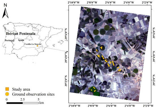
Figure 1.
Location of the study area and distribution of ground sampling point. On the right is the composite image of compact high-resolution imaging spectrometer (CHRIS) data at 461 nm, 562 nm, and 642 nm.
In the Sentinel-3 Experiment, the ground measurements were conducted from 20 June 2009 to 24 June 2009 for agricultural parameter data collection. The ground data acquisition method was designed to ensure that the data represented the crop variability in the experimental area, while minimizing field sampling (for more details, please refer to the report on the Sentinel-3 Experimental Campaign [57]). The LAI of 46 elementary sampling units (ESUs) was obtained simultaneously using the LAI-2000 plant canopy analyzer and NIKON camera with a FC-E8 fisheye, and 42 of these samples were valid (i.e., ESUs with complete parameter measurements and reasonable standard deviation in repeated measurements); the leaf chlorophyll content (LCC) of 51 ESUs was obtained using a SPAD-502 chlorophyll analyzer, and 44 of these samples were valid (see the work by Jesús Delegido [78] for specific details on the treatment). The leaf equivalent water thickness (EWT) was determined by measuring the difference between the dry and fresh weight of the sample (the sample consists of about 5% stems and 95% leaves) and then dividing by the sample area. The size of each ESU was 20 m × 20 m, which generally included a resampled CHRIS pixel. In each ESU, the sampling strategy was based on the VALERI methodology (http://w3.avignon.inra.fr/valeri/). Five pixels that intersected each ESU were averaged to calculate the representative information of CHRIS reflectance [25,27,79]. The position of each ESU in the experimental area is shown in Figure 1. The statistics of the biophysical and biochemical parameters of various crop samples are shown in Table 2 and basically follow a Gaussian distribution.
Table 2.
Statistics of main biophysical and biochemical parameters measured in Sentinel-3 Experiment.
2.5. LAI Inversion Flow Chart
The LAI estimation process is shown in Figure 2. First, based on the variable combinations in Table 1, simulated canopy spectral data (spectral range 450–2500 nm, sampling interval 1 nm) were generated using the PROSAIL model. The simulated CHRIS spectral dataset was then generated according to the simulated canopy spectra data and the CHRIS’s spectral response function. Next, features were extracted from the simulated CHRIS spectrum using the PLS algorithm and the feature components from PLS, and the algorithms mentioned in Section 2.3 were used to construct the LAI inversion model.
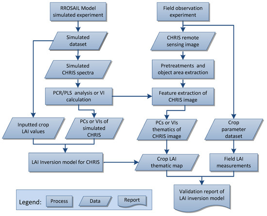
Figure 2.
Flow chart of LAI estimation in this study.
Finally, the LAI inversion model was validated using the field observations described in Section 2.4. At this stage, the crop coverage of the study area was extracted with the normalized difference vegetation index (NDVI) threshold method, and then the true CHRIS data were analyzed using the conversion matrix obtained from the PLS analysis on the CHRIS spectrum. PCs of the true CHRIS data and hybrid inversion model were then used for mapping to obtain the LAI thematic map. For each sampling site, the LAI values estimated by the model were validated against the measurements. The estimation method based on VIs was used for comparative analysis. The data process was completed by using MATLAB 7.10 (MathWorks, Inc., Natick, MA, USA) and Unscrambler 10.3 (Camo Analytics, Inc. Gaustadalléen, Oslo, Norway).
3. Results and Analysis
3.1. Spectral Feature Information Extraction for LAI Estimation
3.1.1. Appropriate PCs for LAI Estimation
PCR and PLS were conducted on the simulations of the training dataset, and the cumulative explained variance contribution rates of the first nine PCs to the dependent variable (i.e., LAI) are shown in Figure 3. The first nine PCs of Specific dataset 1 and Specific dataset 2 contributed approximately 90% of the variance and contained most of the feature information (in both the PCR and PLS models); however, those of the Generic dataset contributed only approximately 80%. These results show that, without prior knowledge constraints on the parameters of the PROSAIL model, the effect of extracting LAI-related features from simulated spectra is relatively poor when both PLS and PCR are used, which may affect the estimation accuracy of the model.
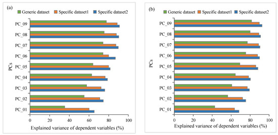
Figure 3.
Cumulative explained variance of the dependent variable (i.e., LAI) of the first nine principal components of the principal component regression (PCR) (a) and partial least squares (PLS models) (b) in different datasets.
When establishing an inversion model, insufficient feature information will be introduced into the model if too few PCs are selected; as a result, the prediction accuracy of the model will be reduced due to underfitting. Redundant information will be introduced into the model if too many PCs are introduced, resulting in overfitting and reduced prediction accuracy. The optimal number of PCs by cross-validation based on the modeling data was determined by selecting the minimum number of PCs without inducing significant changes in the cumulative reliability (cumulative variance contribution). Figure 3 shows that each model had inflection points at the sixth PC and the first six PCs could explain most of the variance in the dependent variables. The subsequent principal component reintroduction model made little contribution to the cumulative variance of the dependent variables. Therefore, the first six PCs were selected to establish the PCR and PLS models, and then the models were validated by 5000 independent simulations of the test subset. The results are shown in Figure 4.
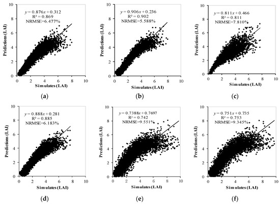
Figure 4.
The PROSAIL model inputted LAI versus the LAI estimated from the PCR/PLS model based on different datasets: (a) PCR based on Specific dataset 2; (b) PLS based on Specific dataset 2; (c) PCR based on Specific dataset 1; (d) PLS based on Specific dataset 1; (e) PCR based on the Generic dataset; and (f) PLS based on the Generic dataset.
As shown in Figure 4, the specific datasets achieved better results than the Generic dataset for both the PCR and PLS models, which indicates that prior knowledge can effectively improve the accuracy of the model. Furthermore, PLS obtained better prediction than the PCR model in both the specific and Generic datasets. This result was achieved because the PLS analysis process combined the information on independent variables and dependent variables and could effectively screen the comprehensive variables with the strongest explanatory power for the dependent variables. Therefore, PLS extracted the LAI-related PCs and achieved a better result than PCR in this paper. In the next step, the PCs extracted by PLS were used to establish the optimization model for LAI inversion using different algorithms. Additionally, due to the presence of random environmental noise in real remote sensing data, the optimal PCs for simulated data may not be the optimal PCs for real remote sensing data. Therefore, the first to sixth PCs were used to establish the LAI inversion model; the optimal PCs were then selected by considering the inversion accuracy and noise immunity.
3.1.2. Selection of Vegetation Indices for LAI Estimation
To screen out optimal VIs for LAI inversion, the simulated LAI values were set as the dependent variables (y), various simulated VIs were set as the independent variables (x), and the curve-fitting models, which selected the optimal models from the linear regression, power regression, exponential regression, logarithmic regression, and quadratic regression were constructed. Then, 5000 independent simulations of the test subset were used for validation. Subsequently, the optimal VIs were chosen according to the method provided by Liang et al. [3,27]. First, the performance of the VIs for LAI estimation in each dataset (i.e., the Generic dataset, Specific dataset 1, and Specific dataset 2) was evaluated by ranking the normalized root-mean-square error (NRMSE) of the validation results in ascending sort order. The integrative performance of the various VIs across the three datasets was then assessed by the comprehensive ranks, which were arranged in ascending sort order.
Using the test subset (5000 simulations) as the data source, the NRMSEs of the validation results constructed by various VIs are shown in Figure 5. The models that utilized the two specific datasets generally yielded lower NRMSEs than those that utilized the Generic dataset, confirming previous studies, which stated that more completely utilizing prior knowledge (e.g., ancillary data measured on site) is an effective method to reduce the estimation error [3,21,52]. VI selection is very important for improving the accuracy of LAI estimations. Three VIs, i.e., optimized soil-adjusted vegetation index (OSAVI), modified triangular vegetation index 2 (MTVI2), and enhanced vegetation index (EVI), appeared at the top of the comprehensive rankings, indicating that they estimated LAI accurately cross the specific and generic datasets. Thus, OSAVI, MTVI2, and EVI were chosen as representative VIs for comparative analysis.
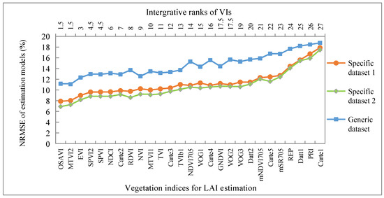
Figure 5.
The normalized root-mean-square error (NRMSE) of the LAI estimation results using the different datasets. The label of the upper x-axis corresponds to the comprehensive ranking (i.e., overall performance) of the various VIs for LAI estimation based on the different datasets. Different VIs with the same number have the same ranking.
The combination of the results presented in Section 3.1.1 and Section 3.1.2 indicates that the accuracy of the model based on Specific dataset 2 was the highest among the three datasets, both when different VIs and when different statistical dimension reduction methods (PCR or PLS) were used to extract spectral features. The accuracy of the model based on Specific dataset 1 was the second highest, but its accuracy was close to that of the model based on Specific dataset 2, while that of the model based on the Generic dataset was the lowest by a considerable margin.
3.2. LAI Inversion Modeling for CHRIS
3.2.1. Model Construction and Anti-Noise Evaluation
Because the models would eventually be applied to the actual remote sensing process, which contains random environmental noise, they were also used to predict the noise samples to evaluate the model’s anti-noise ability. Figure 6 shows the original spectra and additive, multiplicative, and mixed noise spectra, which were generated according to the method described in Section 2.1. After the addition of noise, the spectral values showed random fluctuations, which represented different types of environmental noise. The optimal VIs and PCs were then screened out through comprehensive consideration of prediction accuracy and noise immunity. Finally, the models were optimized using the new machine learning algorithms, such as BP-ANN, SVR, and RFR. The modeling results are shown in Table 3.
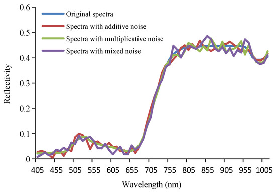
Figure 6.
The original simulated CHRIS spectra and the spectra with additive, multiplicative, and mixed noise. The additive noise with a standard deviation of 0.01; the multiplicative noise with a ratio of 3%; the mixed noise that was a combination of additive noise (with a standard deviation of 0.01) and multiplicative noise (with a ratio of 3%).
Table 3.
LAI prediction and anti-noise analysis results of various modeling methods for independent validation samples (n = 5000). Bold represents the selected objects.
The model estimation accuracy based on a sufficient number of PLS_PCs (i.e., greater than four PCs in this paper) was higher than that based on the optimal VI (i.e., OSAVI in this paper), as indicated by the high R2 and low NRMSE in the prediction datasets (Table 3). The results show that, compared with the VIs, the model constructed using a sufficient number of PCs utilized the spectral information fully and achieved more accurate LAI estimation. However, to estimate LAI, both high accuracy and good anti-noise ability of the model were required. The model based on the optimal VI (i.e., OSAVI in this paper) and appropriate number of PLS_PCs (i.e., four PCs in this paper) achieved a high accuracy of LAI estimation considering both the accuracy and anti-noise ability of the model (Table 3). Nevertheless, the models based on VIs had good anti-noise ability for only multiplicative noise, while they had weak anti-noise ability for additive and mixed noise. After the addition of random additive noise (with a standard deviation of 0.01) or mixed noise (which consisted of additive noise with a standard deviation of 0.01 and multiplicative noise with a ratio of 3%), the estimation accuracies of the models based on OSAVI, MTVI2, and EVI decreased sharply, especially that of the model based on MTVI2. Compared with the models established by the VIs, the model based on the first four PLS_PCs had better noise immunity, as indicated by the small decline in R2 and increase in the NRMSE when the models were used to predict the noise samples. In PLS, the PCs were arranged by ranking the eigenvalues in descending order, in which the first few PCs mainly contained the spectral characteristic information related to LAI and the last few PCs mainly contained the noise information. In this paper, the first four PCs, including characteristic information related to LAI, were used for modeling and the PCs of the noisy information were discarded; therefore, good noise immunity was achieved. The results indicate that the use of appropriate PCs to construct the inversion model was the preferred method for LAI estimation.
Various modeling algorithms exhibited different sensitivity to noise. Compared with the PLS, SVR, and RFR algorithms, the BP-ANN algorithm was more sensitive to noise (Table 3). Although good prediction results were obtained in the noise-free simulation dataset, after the addition of noise, the BP-ANN model exhibited a significant decrease in the prediction accuracy for the different datasets (the Generic dataset and Specific dataset 1 and Specific dataset 2) and different feature extraction methods (VIs and PLS), as indicated by the relatively large decline in R2 and increase in the NRMSE. Moreover, according to Table 3, RFR had higher fitting and prediction accuracy than PLS, BP-ANN, and SVR, as indicated by the lower NRMSE and higher R2. Therefore, in general, the RFR algorithm had good predictability and good noise immunity and was the priority option for modeling. The conclusion was consistent with the previous studies, namely, that RFR can be used as a powerful alternative to other regression algorithms [27,80,81].
In addition, if the influences of the regression algorithm and the number of PCs (or the type of VI) used for modeling were not considered, the order of the modeling accuracies of the three datasets from high to low was Specific dataset 2, Specific dataset 1, and the Generic dataset, as indicated by the changes in the R2 and NRMSE of the model based on these datasets. As shown in Table 1, the utilization of prior knowledge in Specific dataset 2 was also the richest among the three datasets, followed by Specific dataset 1 and finally the Generic dataset. This result shows that the use of more prior knowledge is an effective way to improve the estimation accuracy [3,21,52]. Furthermore, compared with the Generic dataset, the models established by Specific dataset 2 and Specific dataset 1 both achieved good accuracies that were obviously higher than that of the model based on the Generic dataset. Table 1 shows that the difference between Specific dataset 1 and the Generic dataset was the formerly used prior knowledge to constrain the range of major vegetation biochemical parameters (LAI, Cab, and Cw); the difference between Specific dataset 2 and Specific dataset 1 was the formerly used prior knowledge to constrain the range of observation geometric parameters (zenith angle, azimuth angle, and altitude angle). The parameters LAI, Cab, and Cw contributed more to the vegetation canopy spectra than the observation geometric parameters [30,82,83]. Therefore, when prior knowledge was used to constrain the range of major vegetation biochemical parameters, the accuracy of the model was improved. This result shows that in LAI estimation, the use of prior knowledge to constrain parameters, such as LAI and Cab, which made important contributions to the spectra, was key to improving the accuracy of the model. This result was also consistent with that reported in Section 3.1; that is, whether different VIs or different statistical dimension reduction methods (PCR or PLS) were used to extract features, the results show that using more prior knowledge can improve the modeling accuracy and constraints on key parameters, such as LAI, Cab, and Cw, are more effective than constraints on other parameters.
3.2.2. The Contribution of Spectral Bands to PCs
PC selection had an important influence on the generalizability of a model. In the simulated data, while changes in certain factors, such as soil background, were taken into consideration, the simulation of random environmental noise was inadequate. At this time, the use of more PCs typically resulted in increased accuracy (Table 3). However, the lower PCs typically contained only a small portion of the characteristic information and they were susceptible to noise. Therefore, when adding random noise in the spectra, these PCs contained more noise information, which lead to a decline in the inversion accuracy if they were introduced into the model. As shown in Table 3, when introducing the fifth principal component (PC5) and the lower PCs into the model, the prediction accuracy of the samples containing noise was greatly reduced compared with that of the model using only the first four PCs. This result occurred because PC5 and its posterior components contained noise information (PC5 and its posterior PCs accounted for less than one percent of the overall feature information); thus, when introduced into the model, these PCs served as an ineffective component and reduced the accuracy.
The analysis showed that the first four PLS_PCs achieved good estimation accuracy and anti-noise ability. To analyze the source of the feature information contained in the first four PCs, the contributions of various spectral bands to these PCs were analyzed. Figure 7 is an X-loading of each spectral band to the first four PCs and can represent the contribution of each band to different PCs. The contribution of various spectral bands to the first and second PCs was similar in the Generic dataset, Specific dataset 1, and Specific dataset 2, i.e., the first PC reflects the information of the near-infrared spectra and the second PC reflects information related to visible light. Since the first and second PCs contained most of the feature information related to LAI (Figure 7), this result meant that the difference in the contribution of each band to PCs was only reflected in the third and fourth PCs, which contained relatively less feature information.
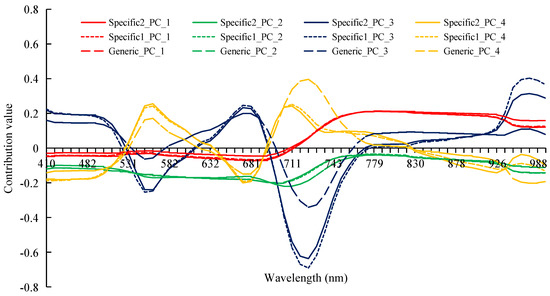
Figure 7.
Contribution of various spectral bands to the first for principal components of different PLS models.
For Specific dataset 1 and Specific dataset 2, the contribution of the various spectral bands to the third and fourth PCs was also similar. As seen from Table 1, the setting of observation geometry parameters in these two data sets was different. Therefore, in the spectral region analyzed in this paper (404.5–1004.5 nm), the values of different observation geometric parameters had little influence on feature extraction with the use of PLS. This finding was consistent with the analysis results in Section 3.2.1; that is, the inversion results of the two datasets were relatively similar. In the Generic dataset, the contribution of the various spectral bands to the third and fourth PCs was somewhat different from the above two datasets in the spectral regions near 560 nm (green peak of vegetation) and 725 nm (red edge of vegetation). This difference was probably caused by the different ranges of the input parameters, such as Cab and LAI, of the Generic dataset. Nevertheless, in all three datasets, these two PCs generally reflected characteristic spectral information of vegetation, such as blue light absorption bands, green peak, red light absorption bands, and the red edge area.
3.3. Model Validation with the CHRIS Data
3.3.1. Image Feature and Crop-Covered Area Extraction
There were two major types of ground objects in the experimental area, namely, dry, bare soil, and farmlands, where various crops were planted but only the crop area was the target. In this study, the NDVI threshold method was used to extract crop growing areas by masking non-crop areas with an NDVI less than 0.25 (Figure 8a). The OSAVI thematic map was then calculated using the masked CHRIS image, and PLS transformation was conducted on true CHRIS images using the transformation matrix obtained from the PLS analysis on a simulated CHRIS spectrum, as described in Section 3.1.1 (Figure 8b).
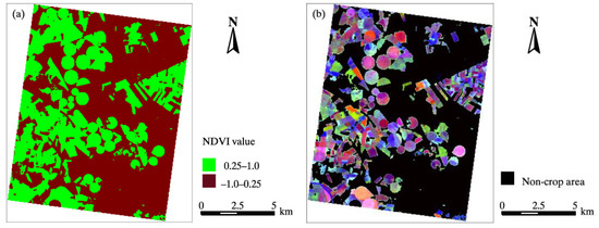
Figure 8.
(a) Crop growing areas of the experimental area and (b) color images of the crop cover area generated using the first three principal components of PLS calculated by Specific dataset 2 conversion matrix (PC_1 for red, PC_2 for green, and PC_3 for blue).
3.3.2. LAI Remote Sensing Mapping and Accuracy Evaluation
The first four PCs and optimal index (OSAVI) obtained from the CHRIS images were used as variables and input into the RFR model established using the simulated data for crop LAI remote sensing mapping (Figure 9). Because the crop LAI is unlikely to be negative, the negative estimation results were assigned to zero. To better realize the visual interpretation of LAI mapping results, they were color-density sliced to six levels of an LAI inversion result. The map provides the spatial information related to crop LAI, which can provide data support for agricultural management.
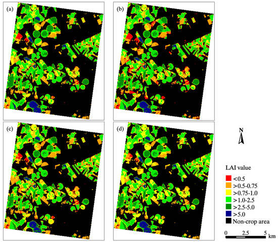
Figure 9.
LAI mapping results of crops from the CHRIS image and various RFR models in Sentinel-3 Experiment: (a) Specific2_PLS_RFR; (b) Specific1_PLS_RFR; (c) Generic_PLS_RFR; (d) Specific2 _OSAVI_RFR.
The accuracy was then validated based on the ground data that were simultaneously collected while the remote sensing image was taken (Figure 10). The LAI values of the 42 sampling sites estimated by the Generic_PLS_RFR model (the RFR model established based on the Generic dataset and PLS feature extraction method) yielded an accuracy of R2 = 0.898 and NRMSE = 8.124%. The Specific1_PLS_RFR model (the RFR model established based on Specific dataset 1 and the PLS feature extraction method), which used prior knowledge to constrain the range of major vegetation biochemical parameters, yielded a higher accuracy (R2 = 0.934 and NRMSE = 7.292%) than the Generic_PLS_RFR model. The Specific2_PLS_RFR model (the RFR model established based on Specific dataset 2 and the PLS feature extraction method), which used prior knowledge to constrain both the major biochemical parameters and observation geometric parameters, yielded an accuracy of R2 = 0.939 and NRMSE = 6.474%, exhibiting the highest accuracy of the three datasets, but the difference from the Specific1_PLS_RFR model was not obvious (Figure 10). This result was consistent with the analysis using the simulated data in Section 3.2; that is, whether simulated or measured data were used, it made better use of prior knowledge to constrain the parameters of the PROSAIL model, especially the key parameters, such as LAI, Cab, and Cw, which can help to obtain more accurate inversion results.
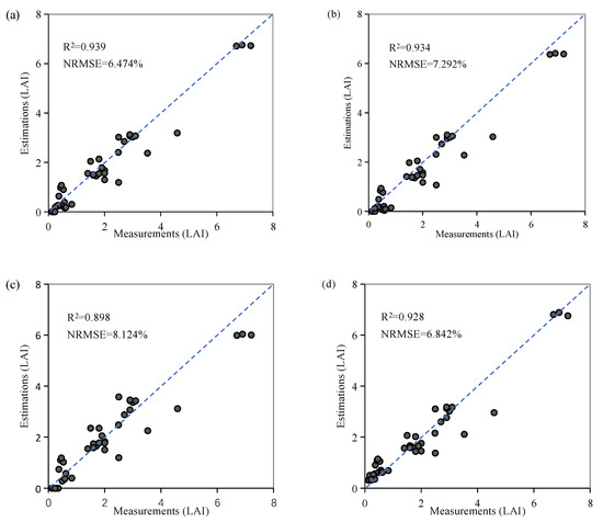
Figure 10.
Ground-measured LAI versus the LAI estimated from the RFR inversion model in the Sentinel-3 Experiment: (a) Specific2_PLS_RFR; (b) Specific1_PLS_RFR; (c) Generic1_PLS_RFR; and (d) Specific2 _OSAVI_RFR.
The optimal VIs can usually obtain good results in vegetation parameter estimation. In this paper, the Specific2_OSAVI _RFR model (the RFR model established based on Specific dataset 2 and the OSAVI) yielded an overall accuracy of R2 = 0.928 and NRMSE = 6.842%. That is, it achieved a high accuracy for crop LAI estimation. Nonetheless, the estimated accuracy was still slightly lower than that of the Specific2_PLS_RFR model, as indicated by the lower R2 and higher NRMSE (Figure 10). In addition, among the above validation data, three data points with high values had an impact on the evaluation index. After removing these three points, R2 of the four validation results in Figure 10 (i.e., Specific2_PLS_RFR, Specific1_PLS_RFR, Generic1_PLS_RFR, and Specific2_OSAVI_RFR) decreased to varying degrees, which were 0.845, 0.836, 0.802, and 0.820, respectively. Nevertheless, the results of comparative analysis were consistent with the above analysis, i.e., Specific2_PLS_RFR had the highest accuracy, followed by Specific1_PLS_RFR (the difference from the Specific1_PLS_RFR was not obvious) and Specific2_OSAVI_RFR, and the Generic1_PLS_RFR model was the lowest.
This result was consistent with the analysis results of the simulated data presented in Section 3.2. This finding indicates that, in both simulated and actual remote sensing, building an inversion model based on the feature information extracted by PLS can obtain the same or even better estimation results as optimal VIs, which is the preferred strategy for LAI inversion modeling.
4. Discussion
In this study, the crop LAI was estimated accurately using a new hybrid inversion method that combined a physical model (i.e., the radiation transfer model) with the regression algorithm. Physical models usually have a general applicability; therefore, in principle, the hybrid method in this study could be applied to different spaceborne and airborne data for similar crop types. Furthermore, unlike empirical models, which require an extensive amount of ground-measured data for modeling, the hybrid inversion method proposed in this paper only needs a few field samples for model assessment [3,15,21]. Compared to other physical model-based strategies (e.g., iterative optimization), the associated calculations of the hybrid inversion method are simple, quick, and accurate, providing a convenient application to real remote sensing for estimating crop parameters [3,26,27,30,84].
The use of the entire band in inversion can make full use of hyperspectral information. However, this approach is computationally complex and prone to interference by factors such as atmospheric moisture absorption, information from the underlying soil, and sunshine conditions when applied to remote sensing data analysis [85,86,87]. In contrast, VIs are simple to calculate and less susceptible to interference factors. Nevertheless, compared with the use of the entire band, VIs contain only part of the effective spectral information, which leads to the loss of information related to the spectral characteristics [16,88,89,90]. Moreover, according to the results of Broge and Leblanc [91] and Liang et al. [3], different vegetation indices are suitable for different conditions, while no universal index is suitable for all conditions. Therefore, the optimization of the VI is important to improve LAI inversion accuracy. This phenomenon, to some extent, complicates the process of LAI inversion using VIs. In this paper, the feature information of hyperspectral data was extracted using PLS dimension reduction and the first four PCs were used as the input variables for modeling. This modeling strategy can reduce the influences of noise interference while fully utilizing the spectral information, avoiding complex index screening processes, and obtaining sufficient or even higher accuracy than the models based on VIs.
Due to the narrow spectral band channel, hyperspectral data are sensitive to random noise; thus, determining how to reduce the impact of random noise is an important aspect of hyperspectral research [92,93,94]. Random noise can be divided into additive noise (independent of wavelength), multiplicative noise (related to wavelength), and additive and multiplicative mixed noise [58,59,60]. Both additive noise (such as thermal noise of the sensor) and multiplicative noise (such as atmospheric disturbance and other environmental changes) are present in remote sensing image data [58,59,60]. In this paper, considering research on the noise of CHRIS data [61,62,63,64], additive noise with a standard deviation of 0.01, multiplicative noise with a proportion of 3%, and mixed noise of the two were used to test the anti-noise ability of the model. The results show that, compared with VI-based model, the PLS-based model showed better anti-noise ability in different noise types. This improvement arose because, compared with the feature factors extracted by PLS, the VIs used only a few wavebands, which are relatively easily affected by random noise [92,93,94,95]. Therefore, the PLS-based estimation model not only had a high inversion accuracy but also a strong anti-noise ability, providing an optimal strategy to estimate a crop’s physical and chemical parameters, such as the LAI.
Combal et al. [52] argued that field-measured data are among the most critical prior knowledge sources. In the present study, the ground-measured data allowed us to more accurately define statistics, such as mean, range, and standard deviation of crop parameters. Therefore, we can reduce the uncertainty of the input parameter of the PROSAIL model, improving the LAI inversion accuracy. In this study the model accuracy based on Specific dataset 2 was shown to be the highest among the three datasets, followed by Specific dataset 1 and, finally, the Generic dataset. These results correspond to the adequacy of the prior knowledge utilized in each dataset and validate the conclusions of previous studies, which indicated that the use of prior knowledge was an effective way to reduce the error of inversion model. The more accurate the prior knowledge is, the higher the inversion accuracy [3,27,91,96]. Furthermore, the results in the study indicated that to improve model accuracy, using prior information to constrain the key parameters, such as LAI and Cab, was more effective than constraints on other parameters (e.g., zenith angle, azimuth angle, and altitude angle). This finding was indicated by the results that the models established using Specific dataset 2 and Specific dataset 1, which both achieved good accuracies that were obviously higher than those obtained by the model based on the Generic dataset.
The selection of the appropriate modeling algorithm can improve LAI inversion accuracy [27,65]. According to Breiman [76] and Polikar [77], the RFR method is simple and robust and thus is preferred for regression models. In the present study, the RFR model showed higher R2 and lower NRMSE values than the PLS, BP-ANN, and SVR models, revealing a higher prediction accuracy. This is consistent with recently published findings [27,31,32,80,84,97]. The RFR algorithm can get good results in various applications, perhaps due to its reasonable hypothesis that different predictors might not be very accurate in different regions, whereas combining the prediction of different predictors can improve the overall prediction accuracy. Therefore, accurate and reliable predictions can be obtained by establishing multiple regression trees for the prediction and then averaging the results of multiple regression trees [76,77].
5. Conclusions
The LAI is a good indicator for crop growth status assessment and health diagnosis. To retrieve this index quickly and accurately over a large scale, a new LAI estimation method was proposed that combines a physical model, spectral feature extraction, and a hybrid inversion strategy. The observation data, including CHRIS remote sensing images and simultaneously measured ground data, were used to validate the inversion results. The validation result indicated that it was feasible to achieve accurate LAI estimation by extracting the feature information of PROSAIL-simulated data by PLS and then constructing the inversion model using the RFR algorithm.
VIs are considered a promising method for estimating vegetation parameters, such as the LAI [3]. Nevertheless, this study showed that using appropriate PCs for modeling is not only as simple and convenient as using VIs but also provides higher precision and stronger anti-noise ability than using VIs for LAI estimation. This result means that the use of PLS to achieve PROSAIL-simulated data reduction and construct the hybrid inversion model can fully combine the advantages of radiation transmission models and empirical models, which is the preferred strategy for LAI estimation.
To reduce the inversion error, it is necessary to select an appropriate modeling algorithm. Compared to PLS, BP-ANN, and LS-SVR algorithms, RFR was the preferred algorithm to establish a regression model of crop LAI estimation, as indicated by its low NRMSE and high R2 for both the generic and specific datasets (Table 3).
Although a model based on physical principles, such as the PROSAIL model, is considered universal to estimate crop physical and chemical parameters, using prior knowledge to constrain model parameters is still necessary. The compared analysis results of the estimation accuracy for various regression algorithms in the Generic dataset, Specific dataset 1, and Specific dataset 2 showed that using prior knowledge was an efficient method for accuracy improvement. Moreover, using prior knowledge to constrain parameters such as LAI and Cab, which provide important contributions to the spectra, is key to improving the model accuracy.
Author Contributions
Conceptualization, L.L. (Liang Liang); methodology, L.L. (Liang Liang); software, G.D., J.Y., S.Q. and L.D.; validation, L.L. (Liang Liang), D.G., J.Y. and S.Q.; formal analysis, D.G. and J.Y.; investigation, D.G., J.Y. and S.Q.; data curation, L.L. (Liang Liang) and L.D.; writing—original draft preparation, L.L. (Liang Liang) and D.G.; writing—review and editing, L.L. (Liang Liang), D.G., J.Y., S.Q., L.X., L.W. and L.L. (Li Li); visualization, S.W. and L.X.; project administration, L.L. (Liang Liang), S.W. and J.K.; funding acquisition, L.L. (Liang Liang), S.W. and J.K. All authors have read and agreed to the published version of the manuscript.
Funding
This research was supported by the Natural Science Foundation of Jiangsu Province (BK20181474), Xuzhou key R&D projects under Grant (KC19134), China Europe Dragon 5 Cooperation Programme (No. 59197), Commissioned Project National Remote Sensing Center of China (No. 2019-NRSCC-019), National Natural Science Foundation of China (No. 41971305), and the Project Funded by the Priority Academic Program Development of Jiangsu Higher Education Institutions (PAPD).
Acknowledgments
The authors wish to thank Yanyan Shi and Zhen Tian from the School of Geography, Geomatics, and Planning, Jiangsu Normal University, China, for their assistance in processing the data. The authors particular thank the ESA for providing the validation data.
Conflicts of Interest
The authors declare no conflict of interest.
Appendix A
Table A1.
Hyperspectral vegetation indices for LAI estimation used in the paper.
Table A1.
Hyperspectral vegetation indices for LAI estimation used in the paper.
| Vegetation Index | Formulation | References |
|---|---|---|
| NDVI705 | [98,99] | |
| mNDVI705 | [100,101] | |
| mSR705 | [100,101] | |
| GNDVI | [102] | |
| RDVI | [103] | |
| NDCI | [104] | |
| Datt1 | [100] | |
| Datt2 | ||
| Carte1 | [105] | |
| Carte2 | ||
| Carte3 | ||
| Carte4 | ||
| Carte5 | ||
| NVI | [106] | |
| EVI | [107,108] | |
| OSAVI | [109] | |
| TVI | [91] | |
| MTVI1 | [90] | |
| MTVI2 | [90] | |
| SPVI | [110,111] | |
| SPVI2 | [111] | |
| REP | [112] | |
| PRI | [113] | |
| VOG1 | [114] | |
| VOG2 | ||
| VOG3 |
Note: DVI705, red edge normalized difference vegetation index; mNDVI705, modified red edge normalized difference vegetation index; mSR705, modified red edge simple ratio index; GNDVI, green normalized difference vegetation index; RDVI, renormalized difference vegetation index; NDCI, normalized difference cloud index; Datt, Datt vegetation index; Carte, Carte vegetation index; NVI, new vegetation index; EVI, enhanced vegetation index; OSAVI, optimized soil-adjusted vegetation index; TVI, triangular vegetation index; MTVI, modified triangular vegetation index; SPVI, spectral polygon vegetation index; REP, red edge position index; PRI, photochemical reflectance index; VOG, Vogelmann red edge index.
References
- Yin, G.; Li, A.; Jin, H.; Zhao, W.; Bian, J.; Qu, Y.; Zeng, Y.; Xu, B. Derivation of temporally continuous LAI reference maps through combining the LAINet observation system with CACAO. Agric. For. Meteorol. 2017, 233, 209–221. [Google Scholar] [CrossRef]
- Kira, O.; Nguy-Robertson, A.L.; Arkebauer, T.J.; Linker, R.; Gitelson, A.A. Informative spectral bands for remote green LAI estimation in C3 and C4 crops. Agric. For. Meteorol. 2016, 218, 243–249. [Google Scholar] [CrossRef]
- Liang, L.; Di, L.; Zhang, L.; Deng, M.; Qin, Z.; Zhao, S.; Lin, H. Estimation of crop LAI using hyperspectral vegetation indices and a hybrid inversion method. Remote Sens. Environ. 2015, 165, 123–134. [Google Scholar] [CrossRef]
- Laurent, V.C.; Schaepman, M.E.; Verhoef, W.; Weyermann, J.; Chávez, R.O. Bayesian object-based estimation of LAI and chlorophyll from a simulated Sentinel-2 top-of-atmosphere radiance image. Remote Sens. Environ. 2014, 140, 318–329. [Google Scholar] [CrossRef]
- Liu, Y.; Ju, W.; Chen, J.; Zhu, G.; Xing, B.; Zhu, J.; He, M. Spatial and temporal variations of forest LAI in China during 2000–2010. Chin. Sci. Bull. 2012, 57, 2846–2856. [Google Scholar] [CrossRef]
- Houborg, R.; Soegaard, H.; Boegh, E. Combining vegetation index and model inversion methods for the extraction of key vegetation biophysical parameters using Terra and Aqua MODIS reflectance data. Remote Sens. Environ. 2007, 106, 39–58. [Google Scholar] [CrossRef]
- Pu, R.; Landry, S. Evaluating seasonal effect on forest leaf area index mapping using multi-seasonal high resolution satellite pléiades imagery. Int. J. Appl. Earth Obs. Geoinf. 2019, 80, 268–279. [Google Scholar] [CrossRef]
- Zhao, C.; Li, H.; Li, P.; Yang, G.; Gu, X.; Lan, Y. Effect of vertical distribution of crop structure and biochemical parameters of winter wheat on canopy reflectance characteristics and spectral indices. IEEE Trans. Geosci. Remote Sens. 2016, 55, 236–247. [Google Scholar] [CrossRef]
- Pu, R.; Cheng, J. Mapping forest leaf area index using reflectance and textural information derived from WorldView-2 imagery in a mixed natural forest area in Florida, US. Int. J. Appl. Earth Obs. Geoinf. 2015, 42, 11–23. [Google Scholar] [CrossRef]
- Wang, D.; Liang, S. Improving LAI mapping by integrating MODIS and CYCLOPES LAI products using optimal interpolation. IEEE J. Sel. Top. Appl. Earth Obs. Remote Sens. 2013, 7, 445–457. [Google Scholar] [CrossRef]
- Fang, H.; Wei, S.; Liang, S. Validation of MODIS and CYCLOPES LAI products using global field measurement data. Remote Sens. Environ. 2012, 119, 43–54. [Google Scholar] [CrossRef]
- Le Maire, G.; Marsden, C.; Verhoef, W.; Ponzoni, F.J.; Seen, D.L.; Bégué, A.; Stape, J.-L.; Nouvellon, Y. Leaf area index estimation with MODIS reflectance time series and model inversion during full rotations of Eucalyptus plantations. Remote Sens. Environ. 2011, 115, 586–599. [Google Scholar] [CrossRef]
- Ryu, C.; Suguri, M.; Umeda, M. Model for predicting the nitrogen content of rice at panicle initiation stage using data from airborne hyperspectral remote sensing. Biosyst. Eng. 2009, 104, 465–475. [Google Scholar] [CrossRef]
- Liang, L.; Yang, M.; Zhang, L.; Lin, H.; Zhou, X. Chlorophyll content inversion with hyperspectral technology for wheat canopy based on support vector regression algorithm. Trans. Chin. Soc. Agric. Eng. 2012, 28, 162–171. [Google Scholar]
- Liang, L.; Huang, T.; Di, L.; Geng, D.; Yan, J.; Wang, S.; Wang, L.; Li, L.; Chen, B.; Kang, J. Influence of different bandwidths on LAI estimation using vegetation indices. EEE J. Sel. Top. Appl. Earth Obs. Remote Sens. 2020, 13, 1494–1502. [Google Scholar] [CrossRef]
- Darvishzadeh, R.; Skidmore, A.; Schlerf, M.; Atzberger, C.; Corsi, F.; Cho, M. LAI and chlorophyll estimation for a heterogeneous grassland using hyperspectral measurements. ISPRS J. Photogramm. Remote Sens. 2008, 63, 409–426. [Google Scholar] [CrossRef]
- Pu, R.; Gong, P. Wavelet transform applied to EO-1 hyperspectral data for forest LAI and crown closure mapping. Remote Sens. Environ. 2004, 91, 212–224. [Google Scholar] [CrossRef]
- Kötz, B.; Schaepman, M.; Morsdorf, F.; Bowyer, P.; Itten, K.; Allgöwer, B. Radiative transfer modeling within a heterogeneous canopy for estimation of forest fire fuel properties. Remote Sens. Environ. 2004, 92, 332–344. [Google Scholar] [CrossRef]
- Lin, H.; Liang, L.; Zhang, L.; Du, P. Wheat leaf area index inversion with hyperspectral remote sensing based on support vector regression algorithm. Trans. Chin. Soc. Agric. Eng. 2013, 29, 139–146. [Google Scholar]
- Verrelst, J.; Camps-Valls, G.; Muñoz-Marí, J.; Rivera, J.P.; Veroustraete, F.; Clevers, J.G.; Moreno, J. Optical remote sensing and the retrieval of terrestrial vegetation bio-geophysical properties—A review. ISPRS J. Photogramm. Remote Sens. 2015, 108, 273–290. [Google Scholar] [CrossRef]
- Verger, A.; Baret, F.; Camacho, F. Optimal modalities for radiative transfer-neural network estimation of canopy biophysical characteristics: Evaluation over an agricultural area with CHRIS/PROBA observations. Remote Sens. Environ. 2011, 115, 415–426. [Google Scholar] [CrossRef]
- Jacquemoud, S.; Verhoef, W.; Baret, F.; Bacour, C.; Zarco-Tejada, P.J.; Asner, G.P.; François, C.; Ustin, S.L. PROSPECT+ SAIL models: A review of use for vegetation characterization. Remote Sens. Environ. 2009, 113, S56–S66. [Google Scholar] [CrossRef]
- Xu, X.; Lu, J.; Zhang, N.; Yang, T.; He, J.; Yao, X.; Cheng, T.; Zhu, Y.; Cao, W.; Tian, Y. Inversion of rice canopy chlorophyll content and leaf area index based on coupling of radiative transfer and Bayesian network models. ISPRS J. Photogramm. Remote Sens. 2019, 150, 185–196. [Google Scholar] [CrossRef]
- Darvishzadeh, R.; Wang, T.; Skidmore, A.; Vrieling, A.; O’Connor, B.; Gara, T.W.; Ens, B.J.; Paganini, M. Analysis of Sentinel-2 and RapidEye for retrieval of leaf area index in a saltmarsh using a Radiative Transfer Model. Remote Sens. 2019, 11, 671. [Google Scholar] [CrossRef]
- Si, Y.; Schlerf, M.; Zurita-Milla, R.; Skidmore, A.; Wang, T. Mapping spatio-temporal variation of grassland quantity and quality using MERIS data and the PROSAIL model. Remote Sens. Environ. 2012, 121, 415–425. [Google Scholar] [CrossRef]
- Verrelst, J.; Malenovský, Z.; Van der Tol, C.; Camps-Valls, G.; Gastellu-Etchegorry, J.-P.; Lewis, P.; North, P.; Moreno, J. Quantifying vegetation biophysical variables from imaging spectroscopy data: A review on retrieval methods. Surv. Geophys. 2019, 40, 589–629. [Google Scholar] [CrossRef]
- Liang, L.; Qin, Z.; Zhao, S.; Di, L.; Zhang, C.; Deng, M.; Lin, H.; Zhang, L.; Wang, L.; Liu, Z. Estimating crop chlorophyll content with hyperspectral vegetation indices and the hybrid inversion method. Int. J. Remote Sens. 2016, 37, 2923–2949. [Google Scholar] [CrossRef]
- Peng, Y.; Gitelson, A.A. Remote estimation of gross primary productivity in soybean and maize based on total crop chlorophyll content. Remote Sens. Environ. 2012, 117, 440–448. [Google Scholar] [CrossRef]
- Botha, E.; Leblon, B.; Zebarth, B.; Watmough, J. Non-destructive estimation of wheat leaf chlorophyll content from hyperspectral measurements through analytical model inversion. Int. J. Remote Sens. 2010, 31, 1679–1697. [Google Scholar] [CrossRef]
- Liang, S. Quantitative Remote Sensing of Land Surfaces; John Wiley & Sons: Hoboken, NJ, USA, 2005; Volume 30. [Google Scholar]
- Liang, L.; Di, L.; Huang, T.; Wang, J.; Lin, L.; Wang, L.; Yang, M. Estimation of leaf nitrogen content in wheat using new hyperspectral indices and a random forest regression algorithm. Remote Sens. 2018, 10, 1940. [Google Scholar] [CrossRef]
- Houborg, R.; McCabe, M.F. A hybrid training approach for leaf area index estimation via Cubist and random forests machine-learning. ISPRS J. Photogramm. Remote Sens. 2018, 135, 173–188. [Google Scholar] [CrossRef]
- Chlingaryan, A.; Sukkarieh, S.; Whelan, B. Machine learning approaches for crop yield prediction and nitrogen status estimation in precision agriculture: A review. Comput. Electron. Agric. 2018, 151, 61–69. [Google Scholar] [CrossRef]
- Gong, P. Inverting a canopy reflectance model using a neural network. Int. J. Remote Sens. 1999, 20, 111–122. [Google Scholar] [CrossRef]
- Fang, H.; Liang, S. A hybrid inversion method for mapping leaf area index from MODIS data: Experiments and application to broadleaf and needleleaf canopies. Remote Sens. Environ. 2005, 94, 405–424. [Google Scholar] [CrossRef]
- Yue, J.; Yang, G.; Tian, Q.; Feng, H.; Xu, K.; Zhou, C. Estimate of winter-wheat above-ground biomass based on UAV ultrahigh-ground-resolution image textures and vegetation indices. ISPRS J. Photogramm. Remote Sens. 2019, 150, 226–244. [Google Scholar] [CrossRef]
- Xu, M.; Liu, R.; Chen, J.M.; Liu, Y.; Shang, R.; Ju, W.; Wu, C.; Huang, W. Retrieving leaf chlorophyll content using a matrix-based vegetation index combination approach. Remote Sens. Environ. 2019, 224, 60–73. [Google Scholar] [CrossRef]
- Cui, B.; Zhao, Q.; Huang, W.; Song, X.; Ye, H.; Zhou, X. A new integrated vegetation index for the estimation of winter wheat leaf chlorophyll content. Remote Sens. 2019, 11, 974. [Google Scholar] [CrossRef]
- Campos-Taberner, M.; García-Haro, F.J.; Camps-Valls, G.; Grau-Muedra, G.; Nutini, F.; Crema, A.; Boschetti, M. Multitemporal and multiresolution leaf area index retrieval for operational local rice crop monitoring. Remote Sens. Environ. 2016, 187, 102–118. [Google Scholar] [CrossRef]
- Paz Pellat, F.; Romero Sanchez, M.E.; Palacios Vélez, E.; Bolaños González, M.; Valdez Lazalde, J.R.; Aldrete, A. Alcances y limitaciones de los índices espectrales de la vegetación: Análisis de índices de banda ancha. Terra Latinoam. 2015, 33, 27–49. [Google Scholar]
- Meng, S.; Huang, L.-T.; Wang, W.-Q. Tensor decomposition and PCA jointed algorithm for hyperspectral image denoising. IEEE Geosci. Remote Sens. Lett. 2016, 13, 897–901. [Google Scholar] [CrossRef]
- Licciardi, G.A.; Chanussot, J. Nonlinear PCA for visible and thermal hyperspectral images quality enhancement. IEEE Geosci. Remote Sens. Lett. 2015, 12, 1228–1231. [Google Scholar] [CrossRef]
- Conforti, M.; Castrignanò, A.; Robustelli, G.; Scarciglia, F.; Stelluti, M.; Buttafuoco, G. Laboratory-based Vis–NIR spectroscopy and partial least square regression with spatially correlated errors for predicting spatial variation of soil organic matter content. Catena 2015, 124, 60–67. [Google Scholar] [CrossRef]
- Le Maire, G.; François, C.; Soudani, K.; Berveiller, D.; Pontailler, J.-Y.; Bréda, N.; Genet, H.; Davi, H.; Dufrêne, E. Calibration and validation of hyperspectral indices for the estimation of broadleaved forest leaf chlorophyll content, leaf mass per area, leaf area index and leaf canopy biomass. Remote Sens. Environ. 2008, 112, 3846–3864. [Google Scholar] [CrossRef]
- Verhoef, W.; Jia, L.; Xiao, Q.; Su, Z. Unified optical-thermal four-stream radiative transfer theory for homogeneous vegetation canopies. IEEE Trans. Geosci. Remote Sens. 2007, 45, 1808–1822. [Google Scholar] [CrossRef]
- Bowyer, P.; Danson, F. Sensitivity of spectral reflectance to variation in live fuel moisture content at leaf and canopy level. Remote Sens. Environ. 2004, 92, 297–308. [Google Scholar] [CrossRef]
- Weiss, M.; Troufleau, D.; Baret, F.; Chauki, H.; Prevot, L.; Olioso, A.; Bruguier, N.; Brisson, N. Coupling canopy functioning and radiative transfer models for remote sensing data assimilation. Agric. For. Meteorol. 2001, 108, 113–128. [Google Scholar] [CrossRef]
- Wang, M. Research of Vegetation Hybrid Inversion with Hyperspectral Data Based on Transform Algorithm; Jiangsu Normal University: Xuzhou, China, 2013; pp. 26–28. [Google Scholar]
- Feret, J.-B.; François, C.; Asner, G.P.; Gitelson, A.A.; Martin, R.E.; Bidel, L.P.; Ustin, S.L.; Le Maire, G.; Jacquemoud, S. PROSPECT-4 and 5: Advances in the leaf optical properties model separating photosynthetic pigments. Remote Sens. Environ. 2008, 112, 3030–3043. [Google Scholar] [CrossRef]
- Atzberger, C. Object-based retrieval of biophysical canopy variables using artificial neural nets and radiative transfer models. Remote Sens. Environ. 2004, 93, 53–67. [Google Scholar] [CrossRef]
- Weiss, M.; Baret, F. Evaluation of canopy biophysical variable retrieval performances from the accumulation of large swath satellite data. Remote Sens. Environ. 1999, 70, 293–306. [Google Scholar] [CrossRef]
- Combal, B.; Baret, F.; Weiss, M.; Trubuil, A.; Mace, D.; Pragnere, A.; Myneni, R.; Knyazikhin, Y.; Wang, L. Retrieval of canopy biophysical variables from bidirectional reflectance: Using prior information to solve the ill-posed inverse problem. Remote Sens. Environ. 2003, 84, 1–15. [Google Scholar] [CrossRef]
- Liu, L.; Wang, J.; Huang, W.; Zhao, C. Detection of leaf and canopy EWT by calculating REWT from reflectance spectra. Int. J. Remote Sens. 2010, 31, 2681–2695. [Google Scholar] [CrossRef]
- Vohland, M.; Jarmer, T. Estimating structural and biochemical parameters for grassland from spectroradiometer data by radiative transfer modelling (PROSPECT + SAIL). Int. J. Remote Sens. 2008, 29, 191–209. [Google Scholar] [CrossRef]
- Darvishzadeh, R.; Skidmore, A.; Schlerf, M.; Atzberger, C. Inversion of a radiative transfer model for estimating vegetation LAI and chlorophyll in a heterogeneous grassland. Remote Sens. Environ. 2008, 112, 2592–2604. [Google Scholar] [CrossRef]
- Bacour, C.; Baret, F.; Béal, D.; Weiss, M.; Pavageau, K. Neural network estimation of LAI, fAPAR, fCover and LAI× Cab, from top of canopy MERIS reflectance data: Principles and validation. Remote Sens. Environ. 2006, 105, 313–325. [Google Scholar] [CrossRef]
- Brockmann, C. Sentinel-3 Experimental Campaign, Final Report; European Space Agency: Paris, France, 2011. [Google Scholar]
- Fu, P.; Sun, Q.; Ji, Z. A spectral-spatial information based approach for the mixed noise estimation from hyperspectral remote sensing images. J. Infrared Millim. Waves 2015, 34, 236–242. [Google Scholar]
- Meola, J.; Eismann, M.T.; Moses, R.L.; Ash, J.N. Modeling and estimation of signal-dependent noise in hyperspectral imagery. Appl. Opt. 2011, 50, 3829–3846. [Google Scholar] [CrossRef] [PubMed]
- Acito, N.; Diani, M.; Corsini, G. Signal-dependent noise modeling and model parameter estimation in hyperspectral images. IEEE Trans. Geosci. Remote Sens. 2011, 49, 2957–2971. [Google Scholar] [CrossRef]
- Shen, Q.; Zhang, B.; Li, J.-S.; Zhang, X.; Zhang, X.-Y. Atmospheric correction for waterbody images acquired by spaceborne hyperspectral sensor CHRIS. Cehui Xuebao/Acta Geod. Cartogr. Sin. 2008, 37, 476–481+488. [Google Scholar]
- Barducci, A.; Guzzi, D.; Marcoionni, P.; Pippi, I. CHRIS-Proba performance evaluation: Signal-to-noise ratio, instrument efficiency and data quality from acquisitions over San Rossore (Italy) test site. In Proceedings of the 3rd ESA CHRIS/Proba Workshop, Frascati, Italy, 21–23 March 2005. [Google Scholar]
- Mannheim, S.; Segl, K.; Heim, B.; Kaufmann, H. Monitoring of lake water quality using hyperspectral CHRIS-PROBA data. In Proceedings of the 2nd CHRIS/PROBA Workshop, Frascati, Italy, 28–30 April 2004; pp. 28–30. [Google Scholar]
- Garcia, J.; Moreno, J. Removal of noises in CHRIS/Proba images: Application to the SPARC campaign data. In Proceedings of the 2nd CHRIS/Proba Workshop, ESA/ERSIN, Frascati, Italy, 28–30 April 2004; pp. 29–33. [Google Scholar]
- Liang, L.; Yang, M.; Deng, K.; Zhang, L.; Lin, H.; Liu, Z. A new hyperspectral index for the estimation of nitrogen contents of wheat canopy. Acta Ecol. Sin. 2011, 31, 6594–6605. [Google Scholar]
- Jolliffe, I. Principal component analysis. Technometrics 2003, 45, 276. [Google Scholar]
- Huemmrich, K.F.; Campbell, P.K.E.; Gao, B.-C.; Flanagan, L.B.; Goulden, M. ISS as a platform for optical remote sensing of ecosystem carbon fluxes: A case study using HICO. IEEE J. Sel. Top. Appl. Earth Obs. Remote Sens. 2017, 10, 4360–4375. [Google Scholar] [CrossRef]
- Henseler, J.; Hubona, G.; Ray, P.A. Using PLS path modeling in new technology research: Updated guidelines. Ind. Manag. Data Syst. 2016, 116, 2–20. [Google Scholar] [CrossRef]
- Mehmood, T.; Bohlin, J.; Snipen, L. A partial least squares based procedure for upstream sequence classification in prokaryotes. IEEE/ACM Trans. Comput. Biol. Bioinform. 2014, 12, 560–567. [Google Scholar] [CrossRef] [PubMed]
- Asner, G.P.; Martin, R.E.; Knapp, D.E.; Tupayachi, R.; Anderson, C.; Carranza, L.; Martinez, P.; Houcheime, M.; Sinca, F.; Weiss, P. Spectroscopy of canopy chemicals in humid tropical forests. Remote Sens. Environ. 2011, 115, 3587–3598. [Google Scholar] [CrossRef]
- Rossel, R.V. Robust modelling of soil diffuse reflectance spectra by “bagging-partial least squares regression”. J. Near Infrared Spectrosc. 2007, 15, 39–47. [Google Scholar] [CrossRef]
- Abdi, H. Partial least squares regression and projection on latent structure regression (PLS Regression). Wiley Interdiscip. Rev. Comput. Stat. 2010, 2, 97–106. [Google Scholar] [CrossRef]
- Haenlein, M.; Kaplan, A.M. A beginner’s guide to partial least squares analysis. Underst. Stat. 2004, 3, 283–297. [Google Scholar] [CrossRef]
- He, Q. Neural Network and Its Application in IR; Graduate School of Library and Information Science, University of Illinois at Urbana-Champaign Spring: Champaign, IL, USA, 1999. [Google Scholar]
- Vapnik, V. Statistical Learning Theory; Wiley-Interscience: New York, NY, USA, 1998. [Google Scholar]
- Breiman, L. Random forests. Mach. Learn. 2001, 45, 5–32. [Google Scholar] [CrossRef]
- Polikar, R. Ensemble based systems in decision making. IEEE Circuits Syst. Mag. 2006, 6, 21–45. [Google Scholar] [CrossRef]
- Delegido, J.; Vergara, C.; Verrelst, J.; Gandía, S.; Moreno, J. Remote Estimation of Crop Chlorophyll Content by Means of High-Spectral-Resolution Reflectance Techniques. Agron. J. 2011, 103, 1834–1842. [Google Scholar] [CrossRef]
- Jonckheere, I.; Fleck, S.; Nackaerts, K.; Muys, B.; Coppin, P.; Weiss, M.; Baret, F. Review of methods for in situ leaf area index determination: Part I. Theories, sensors and hemispherical photography. Agric. For. Meteorol. 2004, 121, 19–35. [Google Scholar] [CrossRef]
- Adam, E.; Mutanga, O.; Abdel-Rahman, E.M.; Ismail, R. Estimating standing biomass in papyrus (Cyperus papyrus L.) swamp: Exploratory of in situ hyperspectral indices and random forest regression. Int. J. Remote Sens. 2014, 35, 693–714. [Google Scholar] [CrossRef]
- Mutanga, O.; Adam, E.; Cho, M.A. High density biomass estimation for wetland vegetation using WorldView-2 imagery and random forest regression algorithm. Int. J. Appl. Earth Obs. Geoinf. 2012, 18, 399–406. [Google Scholar] [CrossRef]
- Thenkabail, P.S.; Lyon, J.G. Hyperspectral Remote Sensing of Vegetation; CRC Press: Boca Raton, FL, USA, 2016. [Google Scholar]
- Vazquez-Cruz, M.; Guzman-Cruz, R.; Lopez-Cruz, I.; Cornejo-Perez, O.; Torres-Pacheco, I.; Guevara-Gonzalez, R. Global sensitivity analysis by means of EFAST and Sobol’methods and calibration of reduced state-variable TOMGRO model using genetic algorithms. Comput. Electron. Agric. 2014, 100, 1–12. [Google Scholar] [CrossRef]
- Wei, C.; Huang, J.; Mansaray, L.R.; Li, Z.; Liu, W.; Han, J. Estimation and mapping of winter oilseed rape LAI from high spatial resolution satellite data based on a hybrid method. Remote Sens. 2017, 9, 488. [Google Scholar] [CrossRef]
- Yuan, Y.; Zhu, G.; Wang, Q. Hyperspectral band selection by multitask sparsity pursuit. IEEE Trans. Geosci. Remote Sens. 2014, 53, 631–644. [Google Scholar] [CrossRef]
- Feng, J.; Jiao, L.; Zhang, X.; Sun, T. Hyperspectral band selection based on trivariate mutual information and clonal selection. IEEE Trans. Geosci. Remote Sens. 2013, 52, 4092–4105. [Google Scholar] [CrossRef]
- Jia, S.; Ji, Z.; Qian, Y.; Shen, L. Unsupervised band selection for hyperspectral imagery classification without manual band removal. IEEE J. Sel. Top. Appl. Earth Obs. Remote Sens. 2012, 5, 531–543. [Google Scholar] [CrossRef]
- Tillack, A.; Clasen, A.; Kleinschmit, B.; Förster, M. Estimation of the seasonal leaf area index in an alluvial forest using high-resolution satellite-based vegetation indices. Remote Sens. Environ. 2014, 141, 52–63. [Google Scholar] [CrossRef]
- Hill, M.J. Vegetation index suites as indicators of vegetation state in grassland and savanna: An analysis with simulated SENTINEL 2 data for a North American transect. Remote Sens. Environ. 2013, 137, 94–111. [Google Scholar] [CrossRef]
- Haboudane, D.; Miller, J.R.; Pattey, E.; Zarco-Tejada, P.J.; Strachan, I.B. Hyperspectral vegetation indices and novel algorithms for predicting green LAI of crop canopies: Modeling and validation in the context of precision agriculture. Remote Sens. Environ. 2004, 90, 337–352. [Google Scholar] [CrossRef]
- Broge, N.H.; Leblanc, E. Comparing prediction power and stability of broadband and hyperspectral vegetation indices for estimation of green leaf area index and canopy chlorophyll density. Remote Sens. Environ. 2001, 76, 156–172. [Google Scholar] [CrossRef]
- Yuan, Q.; Zhang, Q.; Li, J.; Shen, H.; Zhang, L. Hyperspectral image denoising employing a spatial–spectral deep residual convolutional neural network. IEEE Trans. Geosci. Remote Sens. 2018, 57, 1205–1218. [Google Scholar] [CrossRef]
- Lu, T.; Li, S.; Fang, L.; Ma, Y.; Benediktsson, J.A. Spectral–spatial adaptive sparse representation for hyperspectral image denoising. IEEE Trans. Geosci. Remote Sens. 2015, 54, 373–385. [Google Scholar] [CrossRef]
- Chen, G.; Qian, S.-E. Denoising of hyperspectral imagery using principal component analysis and wavelet shrinkage. IEEE Trans. Geosci. Remote Sens. 2010, 49, 973–980. [Google Scholar] [CrossRef]
- Dechant, B.; Ryu, Y.; Kang, M. Making full use of hyperspectral data for gross primary productivity estimation with multivariate regression: Mechanistic insights from observations and process-based simulations. Remote Sens. Environ. 2019, 234, 111435. [Google Scholar] [CrossRef]
- Meroni, M.; Colombo, R.; Panigada, C. Inversion of a radiative transfer model with hyperspectral observations for LAI mapping in poplar plantations. Remote Sens. Environ. 2004, 92, 195–206. [Google Scholar] [CrossRef]
- Li, Z.; Wang, J.; Tang, H.; Huang, C.; Yang, F.; Chen, B.; Wang, X.; Xin, X.; Ge, Y. Predicting grassland leaf area index in the meadow steppes of northern china: A comparative study of regression approaches and hybrid geostatistical methods. Remote Sens. 2016, 8, 632. [Google Scholar] [CrossRef]
- Gitelson, A.; Merzlyak, M.N. Spectral reflectance changes associated with autumn senescence of Aesculus hippocastanum L. and Acer platanoides L. leaves. Spectral features and relation to chlorophyll estimation. J. Plant Physiol. 1994, 143, 286–292. [Google Scholar] [CrossRef]
- Gitelson, A.; Merzlyak, M.N. Quantitative estimation of chlorophyll-ausing reflectance spectra: Experiments with autumn chestnut and maple leaves. J. Photochem. Photobiol. B Biol. 1994, 22, 247–252. [Google Scholar] [CrossRef]
- Datt, B. A new reflectance index for remote sensing of chlorophyll content in higher plants: Tests using Eucalyptus leaves. J. Plant. Physiol. 1999, 154, 30–36. [Google Scholar] [CrossRef]
- Sims, D.A.; Gamon, J.A. Relationships between leaf pigment content and spectral reflectance across a wide range of species, leaf structures and developmental stages. Remote Sens. Environ. 2002, 81, 337–354. [Google Scholar] [CrossRef]
- Gitelson, A.A.; Kaufman, Y.J.; Merzlyak, M.N. Use of a green channel in remote sensing of global vegetation from EOS-MODIS. Remote Sens. Environ. 1996, 58, 289–298. [Google Scholar] [CrossRef]
- Roujean, J.-L.; Breon, F.-M. Estimating PAR absorbed by vegetation from bidirectional reflectance measurements. Remote Sens. Environ. 1995, 51, 375–384. [Google Scholar] [CrossRef]
- Marshak, A.; Knyazikhin, Y.; Davis, A.; Wiscombe, W.; Pilewskie, P. Cloud-vegetation interaction: Use of normalized difference cloud index for estimation of cloud optical thickness. Geophys. Res. Lett. 2000, 27, 1695–1698. [Google Scholar] [CrossRef]
- Carter, G.A. Ratios of leaf reflectances in narrow wavebands as indicators of plant stress. Remote Sens. 1994, 15, 697–703. [Google Scholar] [CrossRef]
- Gupta, R.; Vijayan, D.; Prasad, T. New hyperspectral vegetation characterization parameters. Adv. Space Res. 2001, 28, 201–206. [Google Scholar] [CrossRef]
- Huete, A.; Liu, H.; Batchily, K.; Van Leeuwen, W. A comparison of vegetation indices over a global set of TM images for EOS-MODIS. Remote Sens. Environ. 1997, 59, 440–451. [Google Scholar] [CrossRef]
- Huete, A.; Justice, C.; Liu, H. Development of vegetation and soil indices for MODIS-EOS. Remote Sens. Environ. 1994, 49, 224–234. [Google Scholar] [CrossRef]
- Rondeaux, G.; Steven, M.; Baret, F. Optimization of soil-adjusted vegetation indices. Remote Sens. Environ. 1996, 55, 95–107. [Google Scholar] [CrossRef]
- Main, R.; Cho, M.A.; Mathieu, R.; O’Kennedy, M.M.; Ramoelo, A.; Koch, S. An investigation into robust spectral indices for leaf chlorophyll estimation. ISPRS J. Photogramm. Remote Sens. 2011, 66, 751–761. [Google Scholar] [CrossRef]
- Vincini, M.; Frazzi, E.; D’Alessio, P. Angular dependence of maize and sugar beet VIs from directional CHRIS/Proba data. In Proceedings of the 4th ESA CHRIS PROBA Workshop, Frascati, Italy, 19–21 September 2006; pp. 19–21. [Google Scholar]
- Clevers, J.G. Imaging spectrometry in agriculture-plant vitality and yield indicators. In Imaging Spectrometry—A Tool for Environmental Observations; Springer: Berlin/Heidelberg, Germany, 1994; pp. 193–219. [Google Scholar]
- Gamon, J.; Penuelas, J.; Field, C. A narrow-waveband spectral index that tracks diurnal changes in photosynthetic efficiency. Remote Sens. Environ. 1992, 41, 35–44. [Google Scholar] [CrossRef]
- Vogelmann, J.; Rock, B.; Moss, D. Red edge spectral measurements from sugar maple leaves. Title Remote Sens. 1993, 14, 1563–1575. [Google Scholar] [CrossRef]


Publisher’s Note: MDPI stays neutral with regard to jurisdictional claims in published maps and institutional affiliations. |
© 2020 by the authors. Licensee MDPI, Basel, Switzerland. This article is an open access article distributed under the terms and conditions of the Creative Commons Attribution (CC BY) license (http://creativecommons.org/licenses/by/4.0/).