Sun-Angle Effects on Remote-Sensing Phenology Observed and Modelled Using Himawari-8

 ,
, 


 and
and 
Abstract
:
1. Introduction
2. Data and Method
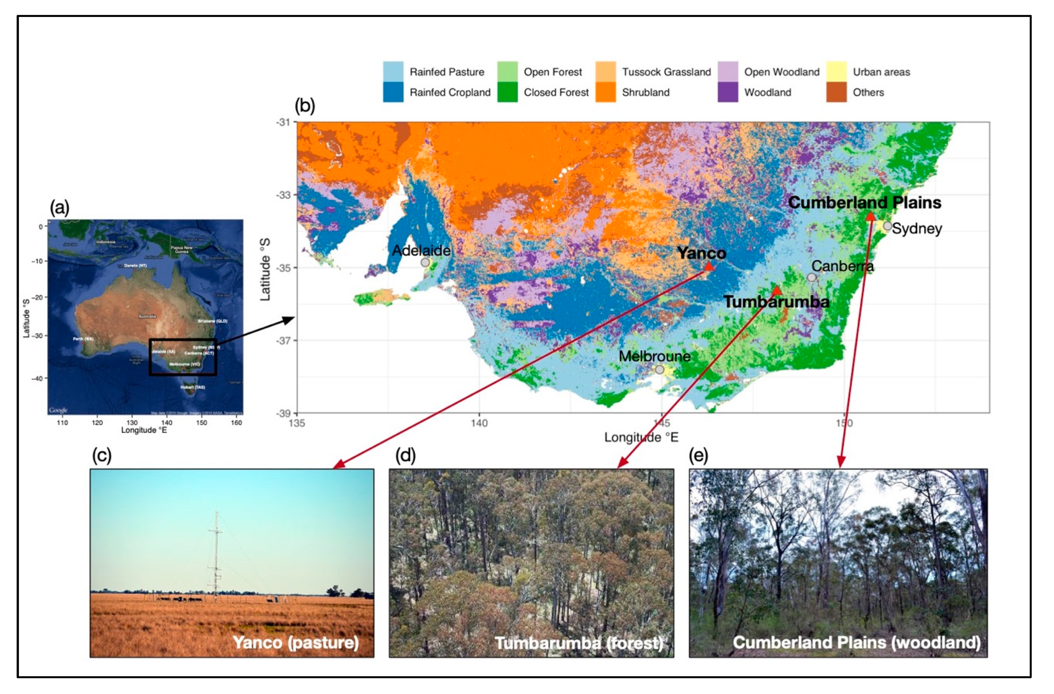
2.1. Study Area
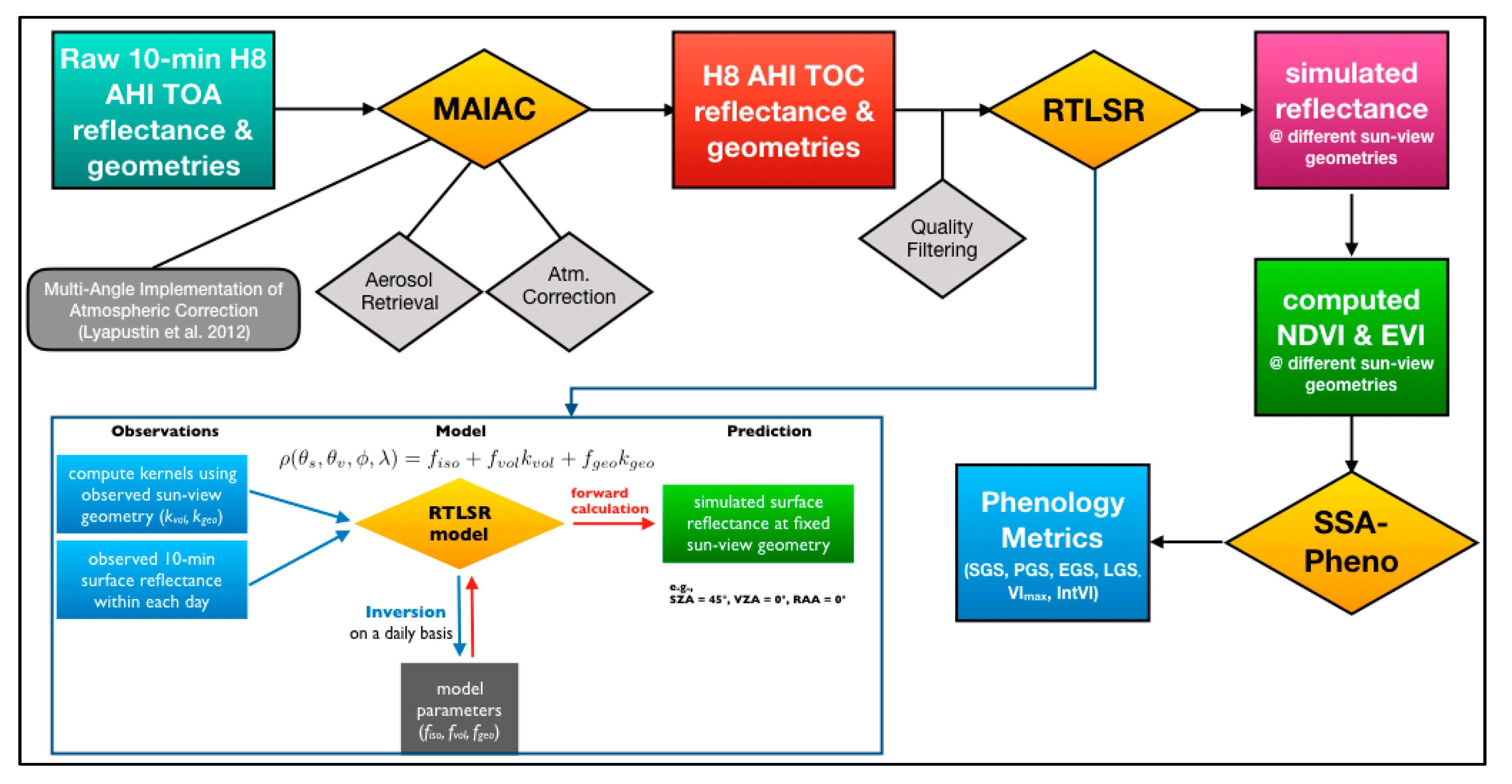
2.2. Himawari-8 Advanced Himawari Imager Data
2.3. Bidirectional Reflectance Distribution Function (BRDF) Modelling
2.4. Vegetation Indices
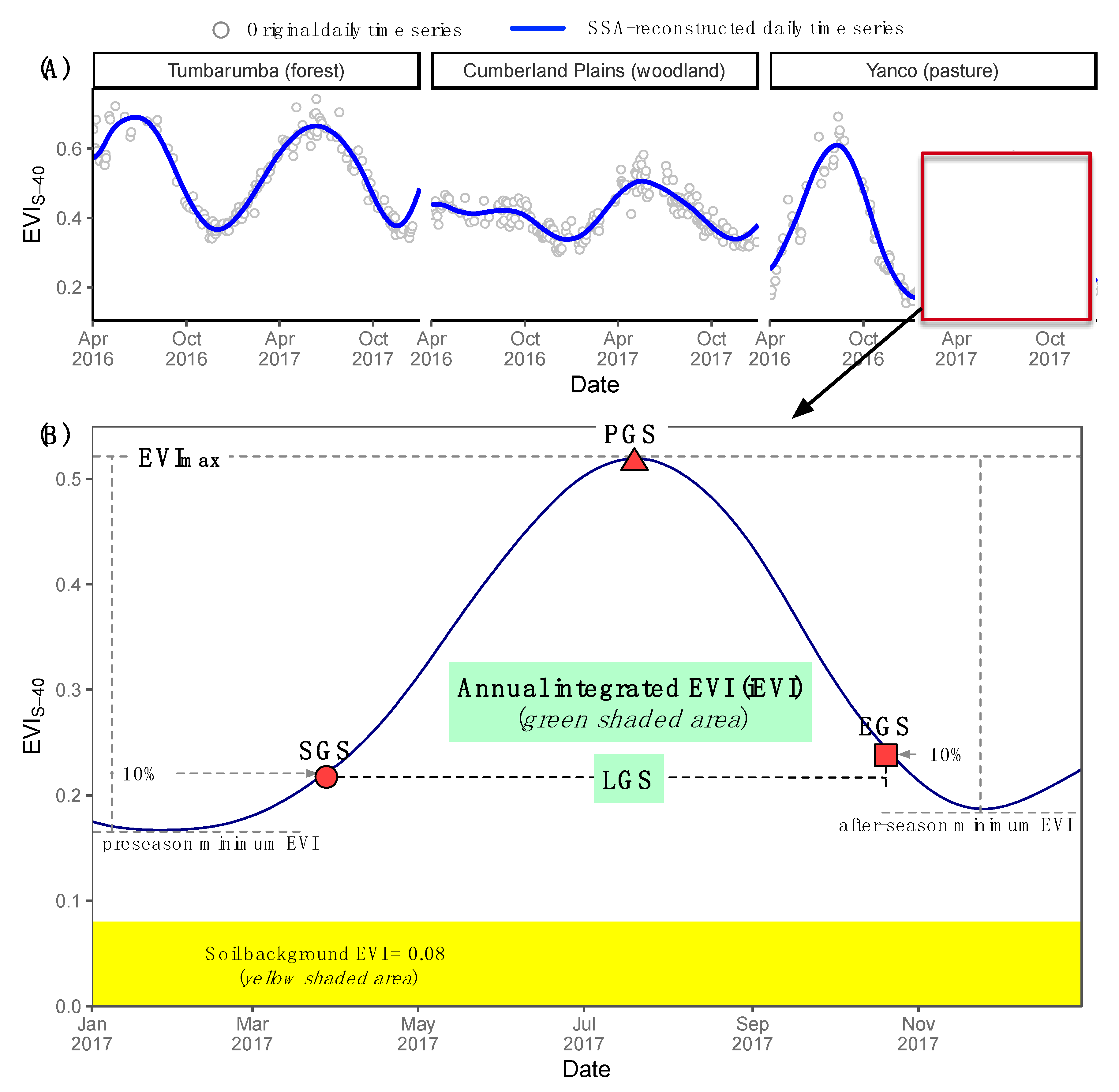
2.5. Phenology Metrics Retrieval Method
2.6. Land-Cover Map
2.7. Statistics
3. Results
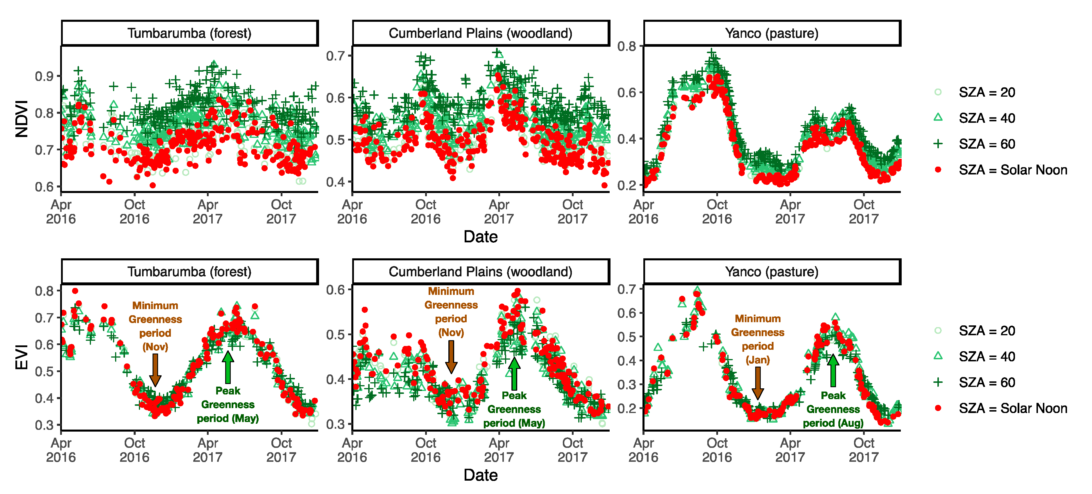
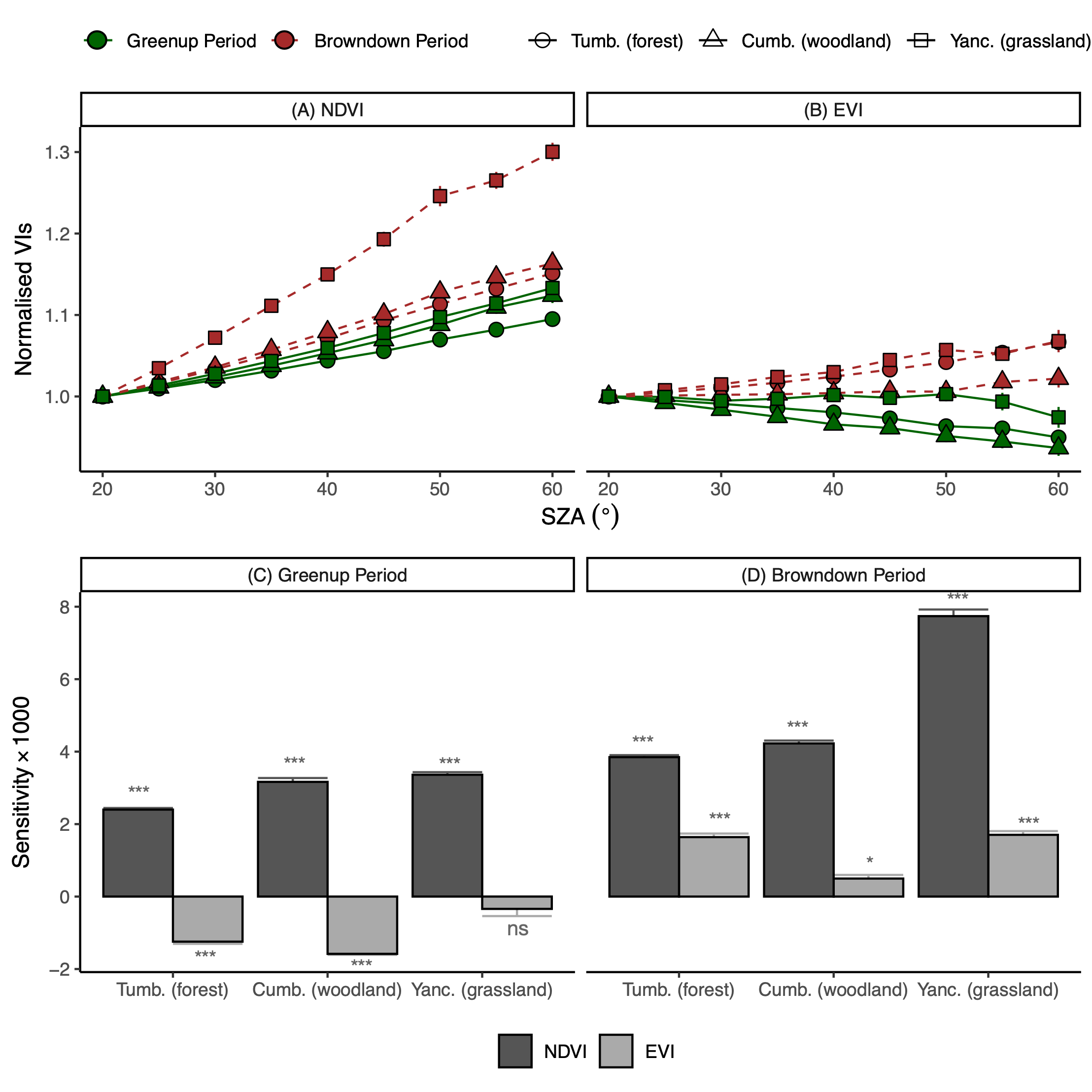
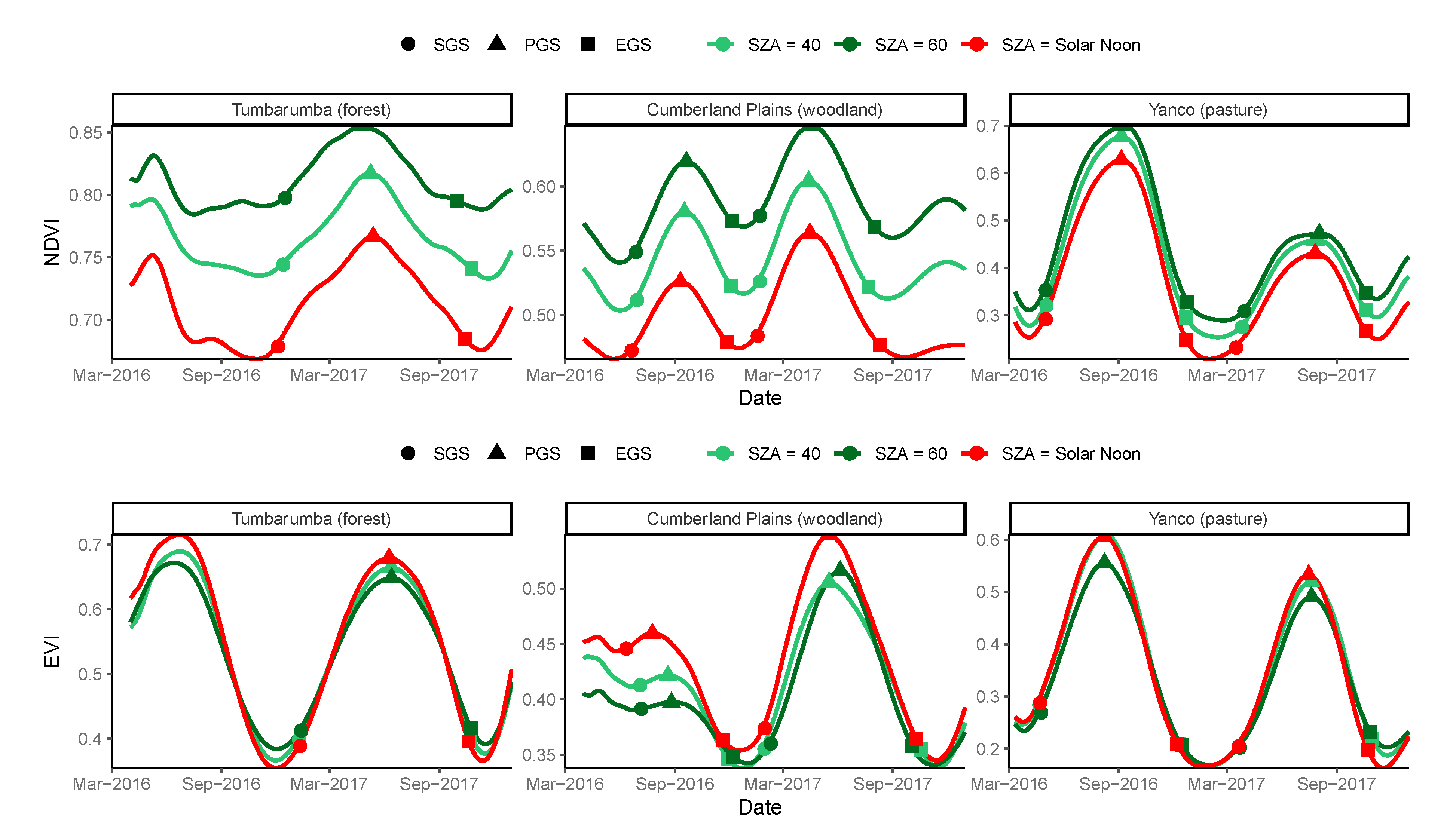
3.1. Seasonal Profiles of Normalized Difference Vegetation Index (NDVI) and Enhanced Vegetation Index (EVI) Normalised to Different Solar Zenith Angles (SZAs)
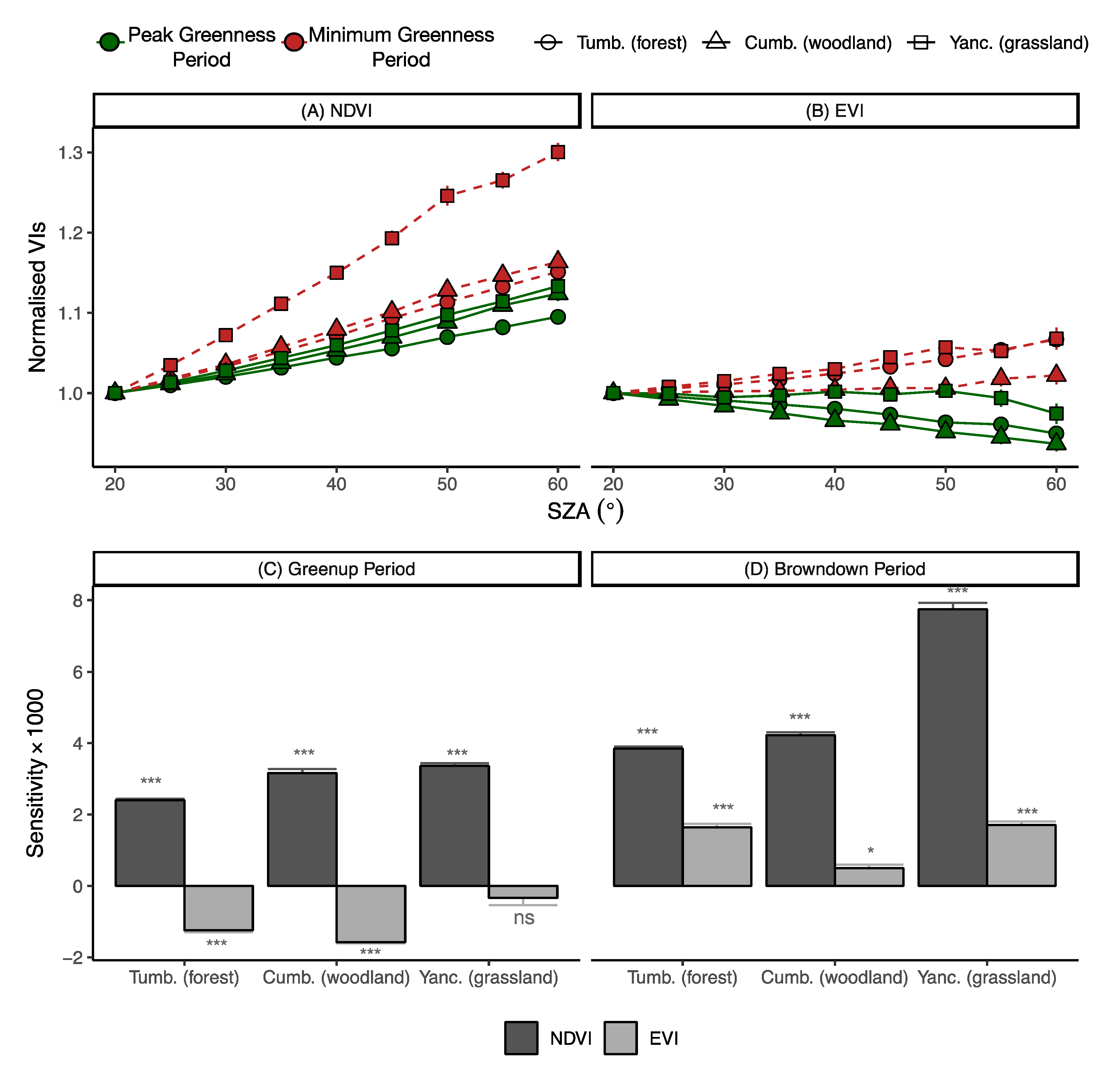
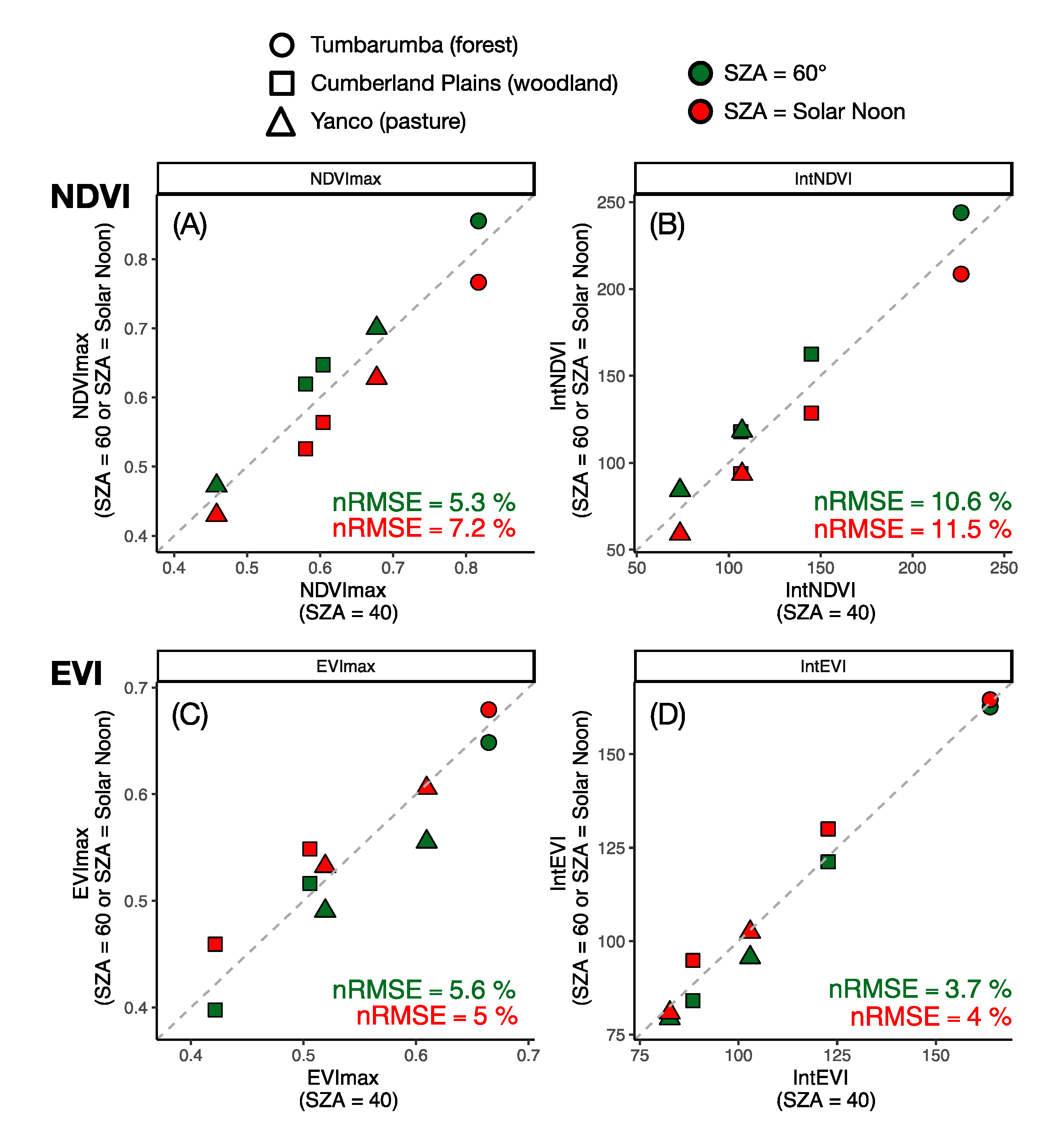
3.2. Sensitivity of NDVI and EVI to Sun-Angle Variations
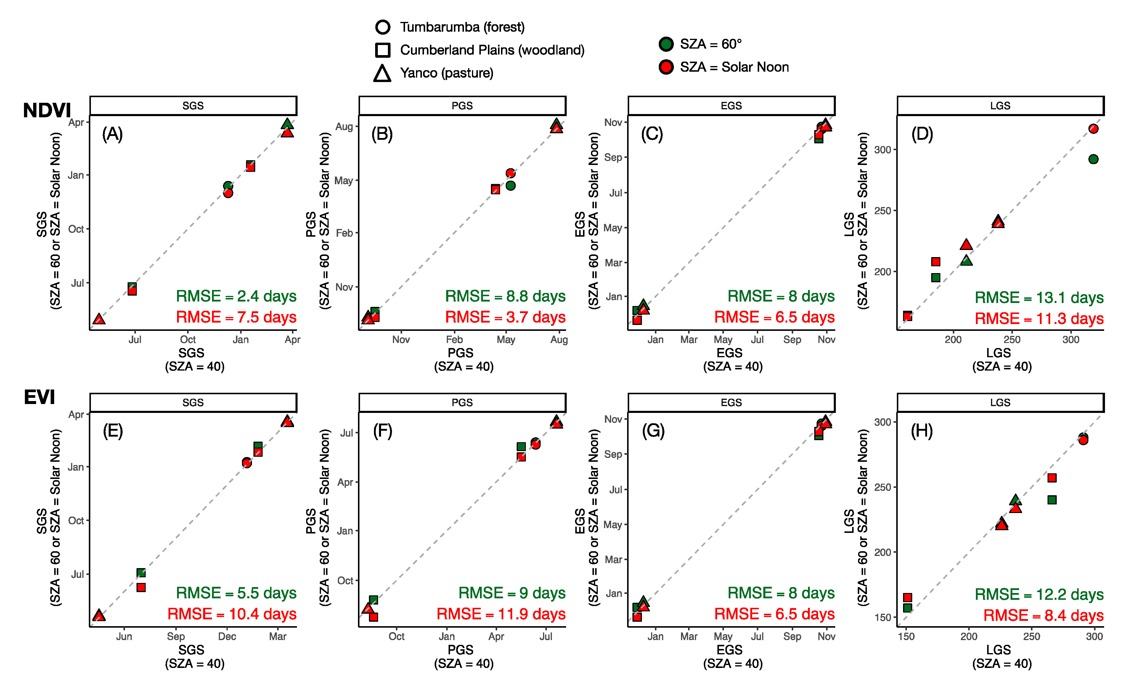
3.3. Sun-Angle Effect on Vegetation Phenology at Site Level
4. Discussion
4.1. Sun-Angle Dependency of Vegetation Indices (VIs)
4.2. Sun-Angle Effect on Retrievals of Vegetation Phenology and Productivity
4.3. Limitations and Future Perspectives
5. Conclusions
Author Contributions
Funding
Acknowledgments
Conflicts of Interest
References
- Pinter, P.J.; Zipoli, G.; Maracchi, G.; Reginato, R.J. Influence of topography and sensor view angles on NIR/red ratio and greenness vegetation indices of wheat. Int. J. Remote Sens. 1987, 8, 953–957. [Google Scholar] [CrossRef]
- Huete, A.R. A Soil-Adjusted Vegetation Index (SAVI). Remote Sens. Environ. 1988, 25, 295–309. [Google Scholar] [CrossRef]
- Kaufman, Y.J.; Tanré, D. Atmospherically Resistant Vegetation Index (ARVI) for EOS-MODIS. IEEE Trans. Geosci. Remote Sens. 1992, 30, 261–270. [Google Scholar] [CrossRef]
- Sellers, P.J.; Tucker, C.J.; Collatz, G.J.; Los, S.O.; Justice, C.O.; Dazlich, D.A.; Randall, D.A. A revised land surface parameterizaton (SiB-2) for atmospheric GCMs. Part 2: The generation of global fields of terrestrial biophysical parameters from satellite data. J. Clim. 1996, 9, 706–737. [Google Scholar] [CrossRef] [Green Version]
- Los, S.O.; North PR, J.; Barnsley GM, J. A methood to convert AVHRR Normalized Difference Vegetation Index time series to a standard viewing and illumination geometry. Remote Sens. Environ. 2005, 99, 400–411. [Google Scholar] [CrossRef]
- Kobayashi, H.; Dye, D.G. Atmospheric conditions for monitoring the long-term vegetation dynamics in the Amazon using normalized difference vegetation index. Remote Sens. Environ. 2005, 97, 519–525. [Google Scholar] [CrossRef]
- Ren, H.; Zhou, G.; Zhang, F. Using negative soil adjustment factor in soil-adjusted vegetation index (SAVI) for aboveground living biomass estimation in arid grassland. Remote Sens. Environ. 2018, 209, 439–445. [Google Scholar] [CrossRef]
- Zhang, Z.; Zhang, Y.; Joiner, J.; Migliavacca, M. Angle matters: Bidirectional effects impact the slope of relationship between gross primary productivity and sun-induced chlorophyll fluorescence from Orbiting Carbon Observatory-2 across biomes. Glob. Chang. Biol. 2018, 24, 5017–5020. [Google Scholar] [CrossRef] [Green Version]
- Jin, Y.; Schaaf, C.B.; Woodcock, C.E.; Gao, F.; Li, X.; Strahler, A.H. Consistency of MODIS surface bidirectional reflectance distribution function and albedo retrievals: 2. Validation. J. Geophys. Res. 2003, 108. [Google Scholar] [CrossRef] [Green Version]
- Gao, F.; He, T.; Masek, J.G.; Shuai, Y.; Schaaf, C.B.; Wang, Z. Angular effects and correction for medium resolution sensors to support crop monitoring. IEEE J. Sel. Top. Appl. Earth Obs. Remote Sens. 2014, 7, 4480–4489. [Google Scholar] [CrossRef]
- Bi, J.; Knyazikhin, Y.; Choi, S.; Park, T.; Barichvich, J.; Ciais, P.; Fu, R.; Ganguly, S.; Hall, F.; Hilker, T.; et al. Sunlight mediated seasonality in canopy structure and photosynthetic activity of Amazonian rainforests. Environ. Res. Lett. 2015, 10, 064014. [Google Scholar] [CrossRef] [Green Version]
- Vermote, E.F.; El Saleous, N.Z.; Justice, C.O. Atmospheric correction of MODIS data in the visible to middle infrared: First results. Remote Sens. Environ. 2002, 83, 97–111. [Google Scholar] [CrossRef]
- Huete, A.; Didan, K.; Miura, T.; Rodriguez, E.P.; Gao, X.; Ferreira, L.G. Overview of the radiometric and biophysical performance of the MODIS vegetation indices. Remote Sens. Environ. 2002, 83, 195–213. [Google Scholar] [CrossRef]
- Schaaf, C.B.; Gao, F.; Strahler, A.H.; Lucht, W.; Li, X.; Tsang, T.; Strugnell, N.C.; Zhang, X.; Jin, Y.; Muller, J.-P.; et al. First operational BRDF, albedo, nadir reflectance products from MODIS. Remote Sens. Environ. 2002, 83, 135–148. [Google Scholar] [CrossRef] [Green Version]
- Cowell, J.E. Vegetation canopy reflectance. Remote Sens. Environ. 1974, 3, 175–183. [Google Scholar] [CrossRef]
- Pinter, P.J.; Jackson, R.D.; Idso, S.B. Diurnal patterns of wheat spectral reflectances. IEEE Trans. Geosci. Remote Sens. 1983, 21, 156–163. [Google Scholar] [CrossRef]
- Huete, A.R. Soil and sun-angle interactions on partial canopy spectra. Int. J. Remote Sens. 1987, 8, 1307–1317. [Google Scholar] [CrossRef]
- Middleton, E.M. Solar zenith angle effects on vegetation indices in tallgrass prairie. Remote Sens. Environ. 1991, 38, 45–62. [Google Scholar] [CrossRef]
- Walter-Shea, E.A.; Biehl, L.L. Measuring vegetation spectral properties. Remote Sens. Rev. 1990, 5, 179–205. [Google Scholar] [CrossRef]
- van Leeuwen, W.J.D.; Huete, A.R.; Laing, T.W. MODIS vegetation index compositing approach: A prototype with AVHRR data. Remote Sens. Environ. 1999, 69, 264–280. [Google Scholar] [CrossRef]
- Petri, C.A.; Galvão, L.S. Sensitivity of seven MODIS vegetation indices to BRDF effects during the Amazonian dry season. Remote Sens. 2019, 11, 1650. [Google Scholar] [CrossRef] [Green Version]
- Schaaf, C.B.; Strahler, A.H. Solar zenith angle effects on forest canopy hemispherical reflectances calculated with a geometric-optical bidirectional reflectance model. IEEE Trans. Geosci. Remote Sens. 1993, 31, 921–927. [Google Scholar] [CrossRef]
- Tucker, C.J.; Pinzon, J.E.; Brown, M.E.; Slayback, D.A.; Pak, E.W.; Mahoney, R.; Vermote, E.F.; El Saleous, N. An extended AVHRR 8-km NDVI dataset compatible with MODIS and SPOT vegetation NDVI data. Int. J. Remote Sens. 2005, 26, 4485–4498. [Google Scholar] [CrossRef]
- Uprety, S.; Cao, C. Suomi NPP VIIRS reflective solar band on-orbit radiometric stability and accuracy assessment using desert and Antarctic Dome C sites. Remote Sens. Environ. 2015, 166, 106–115. [Google Scholar] [CrossRef]
- Bhandari, S.; Phinn, S.; Gill, T. Assessing viewing and illumination geometry effects on the MODIS vegetation index (MOD13Q1) time series: Implications for monitoring phenology and disturbances in forest communities in Queensland, Australia. Int. J. Remote Sens. 2014, 32, 7513–7538. [Google Scholar] [CrossRef]
- Galvão, L.S.; Breunig, F.M.; dos Santos, J.R.; de Moura, Y.M. View-illumination effects on hyperspectral vegetation indices in the Amazonian tropical forest. Int. J. Appl. Earth Obs. Geoinf. 2013, 21, 291–300. [Google Scholar] [CrossRef]
- Morton, D.C.; Nagol, J.; Carabajal, C.C.; Rosette, J.; Palace, M.; Cook, B.D.; Vermote, E.F.; Harding, D.J.; North, P.R.J. Amazon forests maintain consistent canopy structure and greenness during the dry season. Nature 2014, 506, 221–224. [Google Scholar] [CrossRef]
- Ma, X.; Huete, A.; Tran, N.N. Interaction of seasonal sun-angle and savanna phenology observed and modelled using MODIS. Remote Sens. 2019, 11, 1398. [Google Scholar] [CrossRef] [Green Version]
- Huete, A.R.; Didan, K.; Shimabukuro, Y.E.; Ratana, P.; Saleska, S.R.; Hutyra, L.R.; Yang, W.; Nemani, R.R.; Myneni, R. Amazon rainforests green-up with sunlight in dry season. Geophys. Res. Lett. 2006, 33. [Google Scholar] [CrossRef] [Green Version]
- Maeda, E.E.; Heiskanen, J.; Aragão, L.E.O.C.; Rinne, J. Can MODIS EVI monitor ecosystem productivity in the Amazon rainforest? Geophys. Res. Lett. 2014, 41, 7176–7183. [Google Scholar] [CrossRef]
- Saleska, S.R.; Wu, J.; Guan, K.; Araujo, A.C.; Huete, A.; Nobre, A.D.; Restrepo-Coupe, N. Dry-season greening of Amazon forests. Nature 2016, 531, E4–E5. [Google Scholar] [CrossRef] [PubMed]
- Wu, J.; Albert, L.P.; Lopes, A.P.; Restrepo-Coupe, N.; Hayek, M.; Wiedemann, K.T.; Guan, K.; Stark, S.C.; Christoffersen, B.; Prohaska, N.B.; et al. Leaf development and demography explain photosynthetic seasonality in Amazon evergreen forests. Science 2016, 351, 972–976. [Google Scholar] [CrossRef] [PubMed] [Green Version]
- Proud, S.R.; Zhang, Q.; Schaaf, C.; Fensholt, R.; Rasmussen, M.O.; Shisanya, C.; Mutero, W.; Mbow, C.; Anyamba, A.; Pak, E.; et al. The normalization of surface anisotropy effects present in SEVIRI reflectances by using the MODIS BRDF method. IEEE Trans. Geosci. Remote Sens. 2014, 52, 6026–6039. [Google Scholar] [CrossRef]
- Fensholt, R.; Sandholt, I.; Stisen, S.; Tucker, C. Analysing NDVI for the African continent using the geostationary meteosat second generation SEVIRI sensor. Remote Sens. Environ. 2006, 101, 212–229. [Google Scholar] [CrossRef]
- Sobrino, J.A.; Julien, Y.; Sòria, G. Phenology estimation from Meteosat second generation data. IEEE J. Sel. Top. Appl. Earth Obs. Remote Sens. 2013, 6, 1653–1659. [Google Scholar] [CrossRef]
- Guan, K.; Medvigy, D.; Wood, E.F.; Caylor, K.K.; Li, S.; Jeong, S.J. Deriving vegetation phenological time and trajectory information over Africa using SEVIRI daily LAI. IEEE Trans. Geosci. Remote Sens. 2013, 52, 1113–1130. [Google Scholar] [CrossRef]
- Yan, D.; Zhang, X.; Yu, Y.; Guo, W. A comparison of tropical rainforest phenology retrieved from geostationary (SEVIRI) and polar-orbiting (MODIS) sensors across the Congo Basin. IEEE Trans. Geosci. Remote Sens. 2016, 54, 4867–4881. [Google Scholar] [CrossRef] [Green Version]
- Xie, Q.; Dash, J.; Huete, A.; Jiang, A.; Yin, G.; Ding, Y.; Peng, D.; Hall, C.C.; Brown, L.; Shi, Y.; et al. Retrieval of crop biophysical parameters from Sentinel-2 remote sensing imagery. Int. J. Appl. Earth Obs. Geoinf. 2019, 80, 187–195. [Google Scholar] [CrossRef]
- Kalluri, S.; Daniels, J.; Gunshor, M.; Lindsey, D.; Schmit, T.; Wu, X. The First Year of Advanced Baseline Imager. In Proceedings of the 2018 IEEE International Geoscience and Remote Sensing Symposium, Valencia, Spain, 22–27 July 2018. [Google Scholar]
- Zhang, Q.; Zhang, Y.; Li, Z.; Li, J.; Zhang, X. The effects of sun-viewer geometry on sun-induced fluorescence and its relationship with gross primary production. In Proceedings of the 2019 IEEE International Geoscience and Remote Sensing Symposium, Yokohama, Japan, 28 July–2 August 2019. [Google Scholar]
- Miura, T.; Nagai, S.; Takeuchi, M.; Ichii, K.; Yoshioka, H. Improved characterisation of vegetation and land surface seasonal dynamics in central Japan with Himawari-8 hypertemporal data. Sci. Rep. 2019, 9, 1–12. [Google Scholar] [CrossRef] [Green Version]
- Li, S.; Wang, W.; Hashimoto, H.; Xiong, J.; Vandal, T.; Yao, J.; Qian, L.; Icchi, K.; Lyapustin, A.; Wang, Y.; et al. First provisional land surface reflectance product from geostationary satellite Himawari-8 AHI. Remote Sens. 2019, 11, 2990. [Google Scholar] [CrossRef] [Green Version]
- Fang, L.; Zhan, X.; Schull, M.; Kalluri, S.; Laszlo, I.; Yu, P.; Carter, C.; Hain, C.; Anderson, M. Evapotranspiration data product from NESDIS GET-D system upgrated for GOES-16 ABI observations. Remote Sens. 2019, 11, 2639. [Google Scholar] [CrossRef] [Green Version]
- Chen, Y.; Sun, K.; Chen, C.; Bai, T.; Park, T.; Wang, W.; Nemani, R.R.; Myneni, R.B. Generation and evaluation of LAI and fPAR products from Himawari-8 Advanced Himawari Imager (AHI) data. Remote Sens. 2019, 11, 1517. [Google Scholar] [CrossRef] [Green Version]
- Wheeler, K.I.; Dietz, M.C. A statistical model for estimating midday NDVI from the geostationary operational environmental satellite (GOES) 16 and 17. Remote Sens. 2019, 11, 2507. [Google Scholar] [CrossRef] [Green Version]
- Bessho, K.; Date, K.; Hayashi, M.; Ikeda, A.; Imai, T.; Inoue, H.; Kumagai, Y.; Miyakawa, T.; Murata, H.; Ohno, T.; et al. An introduction to Himawari-8/9-Japan’s new-generation geostationary meteorological satellites. J. Meteorol. Soc. Jpn. 2016, 94, 151–183. [Google Scholar] [CrossRef] [Green Version]
- Beringer, J.; Hutley, L.B.; McHugh, I.; Arndt, S.K.; Campbell, D.; Cleugh, H.A.; Cleverly, J.; de Dios, V.R.; Eamus, D.; Evans, B. An introduction to the Australian and New Zealand flux tower network-OzFlux. Biogeosciences 2016, 13, 5895–5916. [Google Scholar] [CrossRef] [Green Version]
- Lyapustin, A.; Wang, Y.; Laszlo, I.; Hilker, T.; Hall, F.; Sellers, P.; Tucker, C.J.; Korkin, S.V. Multi-Angle Implementation of Atmospheric Correction for MODIS (MAIAC): 3. Atmospheric Correction. Remote Sens. Environ. 2012, 127, 385–393. [Google Scholar] [CrossRef]
- Lyapustin, A.; Wang, Y. MAIAC-Multi-Angle Implementation of Atmospheric Correction for MODIS: Algorithm Theoretical Basis Document, v1.0. 2008. Available online: https://ladsweb.modaps.eosdis.nasa.gov/missions-and-measurements/modis/MAIAC_ATBD_v1.pdf (accessed on 27 February 2020).
- Matsuoka, M.; Honda, R.; Nonomura, A.; Moriya, H.; Akatsuka, S.; Yoshioka, H.; Takagi, M. A method to improve geometric accuracy of Himawari-8/AHI “Japan Area” data. J. Jpn. Soc. Photogramm. Remote Sens. 2016, 54, 280–289. [Google Scholar]
- Lucht, W.; Schaaf, C.B.; Strahler, A.H. An algorithm for the retrieval of albedo from space using semiempirical BRDF models. IEEE Trans. Geosci. Remote Sens. 2000, 38, 977–997. [Google Scholar] [CrossRef] [Green Version]
- Lucht, W.; Roujean, J.L. Considerations in the parametric modeling of BRDF and albedo from multiangular satellite sensor observations. Remote Sens. Rev. 2000, 18, 343–379. [Google Scholar] [CrossRef]
- Roujean, J.L.; Leroy, M.; Deschamps, P.Y. A bidirectional reflectance model of the Earth’s surface for the correction of remote sensing data. J. Geophys. Res. 1992, 97, 20455–20468. [Google Scholar] [CrossRef]
- Li, X.; Strahler, A.H. Geometric-optical bidirectional reflectance modeling of the discrete crown vegetation canopy: Effect of crown shape and mutual shadowing. IEEE Trans. Geosci. Remote Sens. 1992, 30, 276–292. [Google Scholar] [CrossRef]
- Strahler, A.H.; Lucht, W.; Schaaf, C.B.; Tsang, T.; Gao, F.; Li, X.; Muller, J.P.; Lewis, P.; Barnsley, M.J. MODIS BRDF/Albedo Product: Algorithm Theoretical Basis Document Versin 5.0. 1999. Available online: https://modis.gsfc.nasa.gov/data/atbd/atbd_mod09.pdf (accessed on 31 March 2020).
- Matsuoka, M.; Takagi, M.; Akatsuka, S.; Honda, R.; Nonomura, A.; Moriya, H.; Yoshioka, H. Bidirectional reflectance modeling of the geostationary sensor Himawari-8/AHI using a kernal-driven BRDF model. ISPRS Ann. Photogramm. Remote Sens. Spat. Inf. Sci. 2016, III-7, 3–8. [Google Scholar] [CrossRef]
- Lucht, W.; Hyman, A.H.; Strahler, A.H.; Barnsley, M.J.; Hobson, P.; Muller, J.P. A comparison of satellite-derived spectral albedos to ground-based broadband albedo measurements modeled to satellite spatial scale for a semidesert landscape. Remote Sens. Environ. 2000, 74, 85–98. [Google Scholar] [CrossRef]
- Wanner, W.; Li, X.; Strahler, A.H. On the derivation of kernels for kernel-driven models of bidirectional reflectance. J. Geophys. Res. 1995, 100, 21077–21089. [Google Scholar] [CrossRef]
- Schaaf, C.B.; Li, X.; Strahler, A.H. Topographic effects on bidirectional and hemispherical reflectances calculated with a geometric-optical canopy model. IEEE Trans. Geosci. Remote Sens. 1994, 32, 1186–1193. [Google Scholar] [CrossRef]
- Zhang, X.; Friedl, M.A.; Schaaf, C.B.; Strahler, A.H.; Hodges, J.C.F.; Gao, F.; Reed, B.C.; Huete, A. Monitoring vegetation phenology using MODIS. Remote Sens. Environ. 2003, 84, 471–475. [Google Scholar] [CrossRef]
- Beck, P.S.A.; Atzberger, C.; Høgda, K.A.; Johansen, B.; Skidmore, A.K. Improved monitoring of vegetation dynamics at very high latitudes: A new method using MODIS NDVI. Remote Sens. Environ. 2006, 100, 321–334. [Google Scholar] [CrossRef]
- Piao, S.; Fang, J.; Zhou, L.; Ciais, P.; Zhu, B. Variations in satellite-derived phenology in China’s temperate vegetation. Glob. Chang. Biol. 2006, 12, 672–685. [Google Scholar] [CrossRef]
- Tan, B.; Morisette, J.; Wolfe, R.; Gao, F.; Nightingale, J.M.; Pedelty, J.; Ederer, G. User Guide for MOD09PHN and MOD15PHN Version 3.0. 2011. Available online: http://citeseerx.ist.psu.edu/viewdoc/download;jsessionid=416AB95FB7EC158E94B0BB21AFC168F9?doi=10.1.1.492.1979&rep=rep1&type=pdf (accessed on 27 February 2020).
- Wu, C.; Gonsamo, A.; Gough, C.M.; Chen, J.M.; Xu, S. Modeling growing season phenology in North American forests using seasonal mean vegetation indices from MODIS. Remote Sens. Environ. 2014, 147, 79–88. [Google Scholar] [CrossRef]
- Myneni, R.; Hall, F.; Sellers, P.; Marshak, A. The interpretation of spectral vegetation indices. IEEE Trans. Geosci. Remote Sens. 1995, 33, 481–486. [Google Scholar] [CrossRef]
- Huete, A.R.; Glenn, E.P. Remote Sensing of Ecosystem. Adv. Environ. Remote Sens. Sens. Algorithms Appl. 2011, 12, 291–320. [Google Scholar]
- Rouse, J.; Haas, R.; Schell, J.; Deering, D. Monitoring vegetation systems in the Great Plains with ERTS. In Third Earth Resources Technology Satellite Symposium. Technical Presentations, Section A; Freden, S.C., Mercanti, E.P., Becker, M., Eds.; NASA SP-351; National Aeronautics and Space Administration: Washington, DC, USA, 1973; Volume I, pp. 309–317. [Google Scholar]
- Ma, X.; Huete, A.; Yu, Q.; Restrepo-Coupe, N.; Davies, K.; Broich, M.; Ratana, P.; Beringer, J.; Hutley, L.B.; Cleverly, J.; et al. Spatial patterns and temporal dynamics in savanna vegetation phenology across the North Australian Tropical Transect. Remote Sens. Environ. 2013, 139, 97–115. [Google Scholar] [CrossRef]
- Ma, X.; Huete, A.; Moran, S.; Ponce-Campos, G.; Eamus, D. Abrupt shifts in phenology and vegetation productivity under climate extremes. J. Geophys. Res. Biogeosci. 2015, 120, 1–17. [Google Scholar] [CrossRef]
- Wang, D.; Liang, S. Singular spectrum analysis for filling gaps and reducing uncertainties of MODIS Land Products. In Proceedings of the IGARSS 2008–2008 IEEE International Geoscience and Remote Sensing Symposium, Boston, MA, USA, 8–11 July 2008. [Google Scholar]
- Aban, J.L.E.; Tateishi, R. Application of Singular Spectrum Analysis (SSA) for the Reconstruction of Annual Phenological Profiles of NDVI Time Series Data. The 24th Proceedings of Asian Association of Remote Sensing, Section 11. Data Processing: Data Fusion. 2004. Available online: https://a-a-r-s.org/proceeding/ACRS2004/Papers/DF204-7.htm (accessed on 31 March 2020).
- Kondrashov, D.; Ghil, M. Spatio-temporal filling of missing points in geophysical datasets. Nonlinear Process. Geophys. 2006, 13, 151–159. [Google Scholar] [CrossRef] [Green Version]
- Ponce-Campos, G.; Moran, M.S.; Huete, A.; Zhang, Y.; Bresloff, C.; Huxman, T.E.; Eamus, E.; Bosch, D.D.; Buda, A.R.; Gunter, S.A.; et al. Ecosystem resilience despite large-scale altered hydroclimatic conditions. Nature 2013, 494, 349–352. [Google Scholar] [CrossRef] [PubMed]
- Zhang, Y.; Moran, M.S.; Nearing, M.A.; Ponce-Campos, G.E.; Huete, A.R.; Buda, A.R.; Bosch, D.D.; Gunter, S.A.; Kitchen, S.G.; McNab, W.H.; et al. Extreme precipitation patterns and reductions of terrestrial ecosystem production across biomes. J. Geophys. Res. Biogeosci. 2013, 118, 148–157. [Google Scholar] [CrossRef]
- Lymburner, A.; Tan, P.; McIntyre, A.; Thankappan, M.; Sixsmith, J. Dynamic Land Cover Dataset Version 2.1. Geoscience Australia, Canberra. 2015. Available online: https://ecat.ga.gov.au/geonetwork/srv/eng/catalog.search#/metadata/83868 (accessed on 23 April 2020).
- R Core Team. R: A Language and Environment for Statistical Computing. In R Foundation for Statistical Computing; R Core Team: Vienna, Austria, 2019. [Google Scholar]
- Huete, A.; Liu, H.; van Leeuwen, W. The use of vegetation indices in forested regions: Issues of linearity and saturation. In Proceedings of the 1997 IEEE International Geoscience and Remote Sensing Symposium, Singapore, 3–8 August 1997; pp. 1966–1968. [Google Scholar]
- Shuai, Y.; Schaaf, C.; Strahler, A.; Liu, J.; Jiao, Z. Quality assessment of BRDF/albedo retrievals in MODIS operational system. Geophys. Res. Lett. 2008, 35. [Google Scholar] [CrossRef]
- de Abelleyra, D.; Verón, S.R. Comparison of different BRDF correction methods to generate daily normalized MODIS 250 m time series. Remote Sens. Environ. 2014, 140, 46–59. [Google Scholar] [CrossRef]
- Wang, Z.; Schaaf, C.B.; Sun, Q.; Shuai, Y.; Román, M.O. Capturing rapid land surface dynamics with Collection V006 MODIS BRDF/NBAR/Albedo (MCD43) products. Remote Sens. Environ. 2018, 207, 50–64. [Google Scholar] [CrossRef]
- Liu, J.; Shang, J.; Qian, B.; Huffman, T.; Zhang, Y.; Dong, T.; Jing, Q.; Martin, T. Crop yield estimation using time-series MODIS data and the effects of cropland masks in Ontario, Canada. Remote Sens. 2019, 11, 2419. [Google Scholar] [CrossRef] [Green Version]
- Yan, D.; Zhang, X.; Nagai, S.; Yu, Y.; Akitsu, T.; Nasahara, K.N.; Ide, R.; Maeda, T. Evaluating land surface phenology from the Advanced Himawari Imager using observations from MODIS and the Phenological Eyes network. Int. J. Appl. Earth Obs. Geoinf. 2019, 79, 71–83. [Google Scholar] [CrossRef]
- Moriondo, M.; Maselli, F.; Bindi, M. A simple model of regional wheat yield based on NDVI data. Eur. J. Agron. 2007, 26, 266–274. [Google Scholar] [CrossRef]
- Kern, A.; Barcza, Z.; Marjanović, H.; Árendás, T.; Fodor, N.; Bónis, P.; Bognár, P.; Lichtenberger, J. Statistical modelling of crop yield in Central Europe using climate data and remote sensing vegetation indeices. Agric. For. Meteorol. 2018, 260, 300–320. [Google Scholar] [CrossRef]
- Kobayashi, H.; Nagai, S.; Kim, Y.; Yang, W.; Ikeda, K.; Ikawa, H.; Nagano, H.; Suzuki, R. In situ observations reveal how spectral reflectance responds to growing season phenology of an open evergreen forest in Alaska. Remote Sens. 2018, 10, 1071. [Google Scholar] [CrossRef] [Green Version]
- Yuan, W.; Chen, Y.; Xia, J.; Dong, W.; Magliulo, V.; Moors, E.; Olesen, J.E.; Zhang, H. Estimating crop yield using a satellite-based light use efficiency model. Ecol. Indic. 2016, 60, 702–709. [Google Scholar] [CrossRef] [Green Version]
- Bhatt, U.S.; Walker, D.A.; Raynolds, M.K.; Bieniek, P.A.; Epstein, H.E.; Comiso, J.C.; Pinzon, J.E.; Tucker, C.J.; Polyakov, I.G. Recent declines in warming and vegetation greening trends over pan-Arctic tundra. Remote Sens. 2013, 5, 4229–4254. [Google Scholar] [CrossRef] [Green Version]
- Zhang, X.; Kondragunta, S.; Ram, J.; Schmidt, C.; Huang, H.C. Near-real-time global biomass burning emissions product from geostationary satellite constellation. J. Geophys. Res. Atmos. 2012, 117. [Google Scholar] [CrossRef]
- Jin, N.; Tao, B.; Ren, W.; Feng, M.; Sun, R.; He, L.; Zhuang, W.; Yu, Q. Mapping irrigated and rainfed wheat areas using multi-temporal satellite data. Remote Sens. 2016, 8, 207. [Google Scholar] [CrossRef] [Green Version]
- Chander, G.; Hewison, T.J.; Fox, N.; Wu, X.; Xiong, X.; Blackwell, W.J. Overview of intercalibration of satellite instruments. IEEE Trans. Geosci. Remote Sens. 2013, 51, 1056–1080. [Google Scholar] [CrossRef]
- Fan, X.; Liu, Y. Multisensor Normalised Difference Vegetation Index intercalibration: A comprehensive overview of the causes of and solutions for multisensor differences. IEEE Geosci. Remote Sens. Mag. 2018, 6, 23–45. [Google Scholar] [CrossRef]
- Qin, Y.; McVicar, T.R. Spectral band unification and inter-calibration of Himawari AHI with MODIS and VIIRS: Constructing virtual dual-view remote sensors from geostationary and low-Earth-orbiting sensors. Remote Sens. Environ. 2018, 209, 540–550. [Google Scholar] [CrossRef]
- Adachi, Y.; Kikuchi, R.; Obata, K.; Yoshioka, H. Relative Azimuthal-Angle Matching (RAM): A screening method for GEO-LEO reflectance comparison in middle latitude forests. Remote Sens. 2019, 11, 1095. [Google Scholar] [CrossRef] [Green Version]
- Grenzdöffer, G.J.; Niemeyer, F. UAV based BRDF-measurements of agricultural surfaces with PFIFFIkus. Int. Arch. Photogramm. Remote Sens. Spat. Inf. Sci. 2011, 38, 229–234. [Google Scholar]
- Baldocchi, D.; Falge, E.; Gu, L.; Olson, R.; Hollinger, D.; Running, S.; Anthoni, P.; Bernhofer, C.; Davis, K.; Evans, R.; et al. FLUXNET: A new tool to study the temporal and spatial variability of ecosystem-scale carbon dioxide, water vapor, and energy flux densities. Bull. Am. Meteorol. Soc. 2001, 82, 2415–2434. [Google Scholar] [CrossRef]
- Aubinet, M.; Vesala, T.; Papale, D. (Eds.) Eddy Covariance: A Practical Guide to Measurement and Data Analysis; Springer: Berlin/Heidelberg, Germany, 2012. [Google Scholar]
- Leuning, R.; Cleugh, H.A.; Zegelin, S.J.; Hughes, D. Carbon and water fluxes over a temperate Eucalyptus forest and a tropical wet/dry savanna in Australia: Measurements and comparison with MODIS remote sensing estimates. Agric. For. Meteorol. 2005, 129, 151–173. [Google Scholar] [CrossRef]
- Cescatti, A.; Marcolla, B.; Santhana Vannan, S.K.; Pan, J.K.; Román, M.O.; Yang, X.; Ciais, P.; Cook, R.B.; Law, B.E.; Matteucci, G.; et al. Intercomparison of MODIS albedo retrievals and in situ measurements across the global FLUXNET network. Remote Sens. Environ. 2012, 121, 323–334. [Google Scholar] [CrossRef] [Green Version]
- Verma, M.; Friedl, M.A.; Law, B.E.; Bonal, D.; Kiely, G.; Black, T.A.; Wohlfahrt, G.; Moors, E.J.; Montagnani, L.; Marcolla, B.; et al. Improving the performance of remote sensing models for capturing intra-and inter-annual variations in daily GPP: An analysis using global FLUXNET tower data. Agric. For. Meteorol. 2015, 214, 416–429. [Google Scholar] [CrossRef] [Green Version]
- Wu, C.; Peng, D.; Soudani, K.; Siebicke, L.; Gough, C.M.; Altaf Arain, M.; Bohrer, G.; Lafleur, P.M.; Peichl, M.; Gonsamo, A.; et al. Land surface phenology derived from normalized difference vegetation index (NDVI) at global FLUXNET sites. Agric. For. Meteorol. 2017, 233, 171–182. [Google Scholar] [CrossRef]
- Gonsamo, A.; Chen, J.M.; Price, D.T.; Kurz, W.A.; Wu, C. Land surface phenology from optical satellite measurements and CO2 eddy covariance technique. J. Geophys. Res. Biogeosci. 2012, 117. [Google Scholar] [CrossRef]
- Zhang, Y.; Xiao, X.; Wu, X.; Zhou, S.; Zhang, G.; Qin, Y.; Dong, J. A global moderate resolution dataset of gross primary production of vegetation for 2000–2016. Sci. Data 2017, 4, 170165. [Google Scholar] [CrossRef] [Green Version]
- Restrepo-Coupe, N.; Huete, A.; Davies, K.; Cleverly, J.; Beringer, J.; Eamus, D.; van Gorsel, E.; Hutley, L.B.; Meyer, W.S. MODIS vegetation products as proxies of photosynthetic potential along a gradient of meteorologically and biologically driven ecosystem productivity. Biogeosciences 2016, 13, 5587–5608. [Google Scholar] [CrossRef] [Green Version]
- Jung, M.; Reichstein, M.; Margolis, H.A.; Cescatti, A.; Richardson, A.D.; Altaf Arain, M.; Arneth, A.; Bernhofer, C.; Bonal, D.; Chen, J.; et al. Global patterns of land-atmosphere fluxes of carbon dioxide, latent heat, and sensible heat derived from eddy covariance, satellite, and meteorological observations. J. Geophys. Res. Biogeosci. 2011, 116. [Google Scholar] [CrossRef] [Green Version]
- Balzarolo, M.; Vicca, S.; Nguy-Robertson, A.L.; Bonal, D.; Elbers, J.A.; Fu, Y.H.; Grünwald, T.; Horemans, J.A.; Papale, D.; Peñuelas, J.; et al. Matching the phenology of Net Ecosystem Exchange and vegetation indices estimated with MODIS and FLUXNET in-situ observation. Remote Sens. Environ. 2016, 174, 290–300. [Google Scholar] [CrossRef] [Green Version]
- Richardson, A.D.; Hollinger, D.Y.; Dail, D.B.; Lee, J.T.; Munger, J.W.; O’keefe, J. Influence of spring phenology on seasonal and annual carbon balance in two contrasting New England forests. Tree Physiol. 2009, 29, 321–331. [Google Scholar] [CrossRef] [PubMed]
- Nasahara, K.N.; Nagai, S. Development of an in situ observation network for terrestrial ecological remote sensing: The Phenological Eyes Network (PEN). Ecol. Res. 2015, 30, 211–223. [Google Scholar] [CrossRef]
- Brown, J.F.; Howard, D.; Wylie, B.; Frieze, A.; Ji, L.; Gacke, C. Application-ready expedited MODIS data for operational land surface monitoring of vegetation condition. Remote Sens. 2015, 7, 16226–16240. [Google Scholar] [CrossRef] [Green Version]
- Wingate, L.; Ogée, J.; Cremonese, E.; Filippa, G.; Mizunuma, T.; Migliavacca, M.; Moisy, C.; Wilkinson, M.; Moureaux, C.; Wohlfahrt, G.; et al. Interpreting canopy development and physiology using the EUROPhen camera network at flux sites. Biogeosciences 2015, 12, 7979–8034. [Google Scholar] [CrossRef] [Green Version]
- Dai, J.; Wang, H.; Ge, Q. The spatial pattern of leaf phenology and its response to climate change in China. Int. J. Biometeorol. 2014, 58, 521–528. [Google Scholar] [CrossRef]


| Site | Longitude (°E) | Latitude (°S) | Elevation (m) | Vegetation Type | MAP * (mm yr−1) | MAT *(°C) |
|---|---|---|---|---|---|---|
| Tumbarumba | 148.1517 | 35.6566 | 1249 | Eucalyptus forest | 1924.2 | 9.6 |
| Cumberland Plains | 150.7236 | 33.6153 | 54 | Eucalyptus woodlands | 806.3 | 18.1 |
| Yanco | 146.2907 | 34.9893 | 128 | Pasture | 472.1 | 17.3 |
| Site | Phenological Stages | δNDVI/δSZA | δEVI/δSZA |
|---|---|---|---|
| Tumbarumba | Peak Greenness Period | 0.0024 | −0.0012 |
| Minimum Greenness Period | 0.0038 | 0.0016 | |
| Cumberland Plains | Peak Greenness Period | 0.0032 | −0.0016 |
| Minimum Greenness Period | 0.0042 | 0.0005 | |
| Yanco | Peak Greenness Period | 0.0034 | −0.0003 |
| Minimum Greenness Period | 0.0077 | 0.0017 |
| Site | Productivity Metrics | SZA Scenarios | NDVI | EVI |
|---|---|---|---|---|
| Tumbarumba | VImax | 40° | 0.82 | 0.66 |
| 60° | 0.86 | 0.65 | ||
| Solar Noon | 0.77 | 0.68 | ||
| IntVI | 40° | 226.54 | 163.77 | |
| 60° | 243.87 | 162.66 | ||
| Solar Noon | 208.56 | 164.63 | ||
| Cumberland Plains | VImax | 40° | 0.59 | 0.46 |
| 60° | 0.63 | 0.46 | ||
| Solar Noon | 0.54 | 0.50 | ||
| IntVI | 40° | 125.72 | 105.58 | |
| 60° | 140.12 | 102.62 | ||
| Solar Noon | 111.19 | 112.42 | ||
| Yanco | VImax | 40° | 0.57 | 0.56 |
| 60° | 0.59 | 0.52 | ||
| Solar Noon | 0.53 | 0.57 | ||
| IntVI | 40° | 90.32 | 92.76 | |
| 60° | 101.22 | 87.47 | ||
| Solar Noon | 76.21 | 91.63 |
© 2020 by the authors. Licensee MDPI, Basel, Switzerland. This article is an open access article distributed under the terms and conditions of the Creative Commons Attribution (CC BY) license (http://creativecommons.org/licenses/by/4.0/).
Share and Cite
Ma, X.; Huete, A.; Tran, N.N.; Bi, J.; Gao, S.; Zeng, Y. Sun-Angle Effects on Remote-Sensing Phenology Observed and Modelled Using Himawari-8. Remote Sens. 2020, 12, 1339. https://doi.org/10.3390/rs12081339
Ma X, Huete A, Tran NN, Bi J, Gao S, Zeng Y. Sun-Angle Effects on Remote-Sensing Phenology Observed and Modelled Using Himawari-8. Remote Sensing. 2020; 12(8):1339. https://doi.org/10.3390/rs12081339
Chicago/Turabian StyleMa, Xuanlong, Alfredo Huete, Ngoc Nguyen Tran, Jian Bi, Sicong Gao, and Yelu Zeng. 2020. "Sun-Angle Effects on Remote-Sensing Phenology Observed and Modelled Using Himawari-8" Remote Sensing 12, no. 8: 1339. https://doi.org/10.3390/rs12081339
APA StyleMa, X., Huete, A., Tran, N. N., Bi, J., Gao, S., & Zeng, Y. (2020). Sun-Angle Effects on Remote-Sensing Phenology Observed and Modelled Using Himawari-8. Remote Sensing, 12(8), 1339. https://doi.org/10.3390/rs12081339