Abstract
Much attention is being paid to using high-performance convolutional neural networks (CNNs) in the area of ship detection in optical remoting sensing (ORS) images. However, the problem of false negatives (FNs) caused by side-by-side ships cannot be solved, and the number of false positives (FPs) remains high. This paper uses a DLA-34 network with deformable convolution layers as the backbone. The network has two priority branches: a recall-priority branch for reducing the number of FNs, and a precision-priority branch for reducing the number of FPs. In our single-shot detection method, the recall-priority branch is based on an anchor-free module without non-maximum suppression (NMS), while the precision-priority branch utilizes an anchor-based module with NMS. We perform recall-priority branch functions based on the output part of the CenterNet object detector to precisely predict center points of bounding boxes. The Bidirectional Feature Pyramid Network (BiFPN), combined with the inference part of YOLOv3, is used to improve the precision of precision-priority branch. Finally, the boxes from two branches merge, and we propose priority-based selection (PBS) for choosing the accurate ones. Results show that our proposed method sharply improves the recall rate of side-by-side ships and significantly reduces the number of false alarms. Our method also achieves the best trade-off on our improved version of HRSC2016 dataset, with 95.57% AP at 56 frames per second on an Nvidia RTX-2080 Ti GPU. Compared with the HRSC2016 dataset, not only are our annotations more accurate, but our dataset also contains more images and samples. Our evaluation metrics also included tests on small ships and incomplete forms of ships.
1. Introduction
Advanced aerospace technologies and optical remote sensing image sensors make it possible to record images of higher resolution over larger areas. Due to the high quality of these remote sensing images, people can complete many tasks and applications that were not possible in the past. For example, Li et al. [1] used remote sensing images to perform urban flood mapping. Sun et al. [2] analyzed the number and locations of cotton bolls based on 3-D photogrammetric mapping. As the importance of ship detection increases in both military and civil use, much research is taking place in this field. In military action and rescue work, detection results can be used to find whether ships exist in a certain area and possibly their exact location. Enhancing the detection accuracy for locating ships is a hot topic worldwide.
Despite the great achievements scientists have made in enabling satellites to provide high-resolution images, partial joggles of images can reduce the accuracy of detection results. Environmental factors, such as ocean waves and severe weather, can also cause the images of ships to suffer from different levels of incompleteness. In addition, the type, color, and material of a ship [3] can also hinder the detection results. Moreover, multi-scale ships and the existence of ship-like floating objects on the sea also negatively affect detection technology. In short, methods to solve the problems involved in ship detection are urgently needed.
The earliest work on ship detection can be traced back to the 1980s when Barnum [4] presented an overview of ship detection by high-frequency skywave backscatter over-the-horizon radar. After that, works on ship detection began to spring up. There are three types of ship detection methods: traditional, machine learning-based, and deep learning-based methods.
In traditional detection, researchers applied mathematical analyses to pixel distribution, statistic data and local gradience. Although high-resolution remote sensing (RS) images can be produced by advanced sensors, such detection is not robust enough for images of different brightness and contrast. Therefore, in traditional method there is pre-processing, including land mask, image enhancement, image segmentation, and false alarm elimination [5]. After processing, Nocak et al. [6] used a global thresholding algorithm to complete ship detection. In the work of Vachon et al. [7], K distribution was used as a marine clutter distribution model. To build a fractal model of ships, Kaplan [8] introduced Hurst parameters and proposed extended fractal features for identifying targets of specific sizes in RS images. Aware of the important role of trails in detecting ships, Copeland et al. [9] described a feature space linear detection method using the local Radon transform to detect trails. However, such methods have weak anti-noise capability, and the detection result depends on the acquisition of prior knowledge.
Detection methods based on machine learning perform better when they rely on noise. One of the most popular algorithms is support vector machine (SVM). According to Dong et al. [3], a trainable Gaussian SVM classifier was performed to validate real ships from ship candidates. Inspired by Bayesian decision theory, Proia et al. [10] fixed the size of the analysis window and the threshold used to make a choice. In addition, histograms of oriented gradient (HOG) feature [11] and binary linear programming [12] were proposed to solve the problem. The machine learning-based methods achieved promising performance and outstanding accuracy [13], but the training process was complicated.
With the recent rapid development of deep learning, researchers are trying to improve the accuracy of detection with the help of convolutional neural networks (CNNs). Lin et al. [14] avoided carefully tuned parameters and complicated procedures by utilizing a full convolution network, which shows ship detection can benefit from CNN. Xie et al. [15] used the reflectance gradient to extract ship candidates and then used LFNet to verify true ships. In this work, ships under complex environment were detected well, but it took extra time to separate ship candidates from the background. Different from [15], Chen et al. [16] proposed an end-to-end structure. It enhanced the segmentation speed compared with their structure without end-to-end connection. In [17], Clément et al. benefited from their large dataset composed of 18,894 raw Synthetic Aperture Radar (SAR) images and achieved good performance in ship detection, classification, and length estimation. Considering the training dataset can be much smaller for other researchers, Dechesne’s method may not work well on other datasets. To get a network which can be effective with only a small labeled dataset, Rostami et al. [18] used an innovative approach to train a DNN for classifying SAR images by transferring knowledge from an electro-optical (EO) domain. Although the method is effective, full overlap was needed between the existing classes across SAR and EO domains. Inspired by the Faster-RCNN detection framework [19], Zhang et al. [20] proved their improved Faster-RCNN could achieve a higher recall and accuracy for small ships and gathering ships. However, ships abreast with each other still cannot be detected easily. To solve the problem, Zhang et al. [21] replaced horizon boxes with inclined ship region proposals. It reduced the rate of misses to an extent, but the calculation of intersection over union (IoU) became more complicated and the method needed more skills to train. Other issues include deep learning’s large amount of training time and the fact that it suffers from overfitting.
For this paper, we conducted several detecting experiments on ORS ship images and discovered the main obstacles that hindered the detection results in previous methods. These obstacles are listed below, and examples of them are shown in Figure 1.
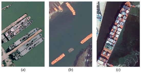
Figure 1.
Main obstacles in ship detection: (a) side-by-side ships; (b) ship-like objects; (c) multi-scale ships.
- Side-by-side ships. In previous works, bounding boxes are produced to cover the area of ships. To avoid repeated bounding boxes on the same ship, researchers apply a non-maximum suppression (NMS) or soft-NMS strategy [22] that prevents bounding boxes from having a large overlap with the most likely box. However, the drawback to this strategy is that if ships are close together, boxes belonging to different ships will be eliminated until down to only one. Therefore, some side-by-side ships will be missed.
- Ship-like objects. Some ship-like objects will be mistaken for ships. This can be attributed to algorithms’ insufficient ability to perform feature extraction, and a lack of negative samples.
- Multi-scale ships. If ships of different sizes gather, the smaller ships are often missed by detectors. Multi-scale outputs are designed to predict ships with different sizes in different modules. This method decreases the number of missed multi-scale ships but does not completely eliminate the possibility of missing them.
We use the CNN algorithm to design a single-shot detector that predicts all bounding boxes and the category at the same time. In our CNN detection method, DLA-34 [23] with deformable convolution layers is used as our backbone. During the detection process, an ORS image is first put into the backbone to create feature maps that contain all the features that the backbone extracts. Then, the feature maps are put into two branches to produce bounding boxes. One branch is the recall-priority branch, which reduces the number of missed side-by-side ships and improves the recall; the other branch distinguishes ship-like objects to increase the precision. In the end, all boxes from the two branches are filtered by priority-based selection (PBS) to obtain boxes with both high recall and high precision. The recall of multi-scale ships is also improved in this process.
Our contributions in this paper include the following:
- A state-of-the-art performance detector is proposed in this paper. Priority branches for CNN ship detectors are specially designed, and PBS is used to filter potential outputs from branches.
- To obtain more samples, we add 360 ORS ship images collected from Google Earth to the HRSC2016 dataset [24]. In our dataset, ships include warcrafts, aircraft carriers, and cargo and passenger ships. We re-annotate the dataset with consistent standards. If a ship is completely displayed in an image, we distinguish whether it is a large ship or a small ship based on whether its bounding box area is larger than 96 × 96 pixels. For those displayed incompletely, we labeled them as incomplete ships. Detecting results of large ships, small ships and incomplete ships are involved in our stricter evaluation metrics.
The code and dataset in this work will be updated to GitHub (https://github.com/Chocolife-96/Priority-Branches-for-Ship-Detection-in-Optical-Remote-Sensing-Images) in the near future.
2. Methodology
The architecture of our proposed priority-based ship detection is shown in Figure 2. It is based on CNN and consists of four parts: a feature fusion backbone; the recall-priority branch, which is an anchor-free module; the precision-priority branch, which is an anchor-based module; and a PBS module. After the ORS image is resized to a resolution of 512 × 512, it goes through the backbone, which integrates the multi-scale feature maps together. Then, the branch functions are performed on the same feature maps produced by the backbone. Finally, boxes from branches are filtered by the PBS to obtain predicted ones.
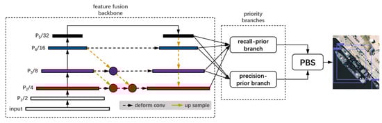
Figure 2.
Our proposed priority-based architecture: DLA-34 using deformable convolution layers is selected as the backbone. Priority branches are used for improving recall rate and precision rate respectively. PBS serves as a bounding box filter which outputs only the accurate boxes we want.
2.1. Feature Fusion Backbone
Our proposed backbone is derived from deep layer aggregation (DLA) and Deformable Convolutional Networks (ConvNets). As an image classification network with hierarchical skip connection [25], DLA has the ability to integrate multi-scale feature maps together. Moreover, deformable convolution derived from Deformable ConvNets v2 is used in up-sample stages, making the convolution process sufficiently robust to work in complex environments.
2.1.1. Deep Layer Aggregation
Aggregation is the combination of different layers throughout a network. Deep layer aggregation (DLA) is when a group of aggregations are compositional and nonlinear, and the earliest layers pass through multiple aggregations. The structure of DLA can be viewed as the connections of blocks which contain several layers. At the same time, blocks are grouped into stages by feature resolution. We select the fully convolutional up-sampling DLA for dense prediction as our backbone, which is a combination of iterative deep aggregation (IDA) and hierarchical deep aggregation (HDA) [23].
The deeper the CNN layers are located, the more semantic they are. However, problems exist. Details would be lost from shallow layers, and as a result the feature maps will be coarse. Unlike the skip connections in previous work, which only integrate the shallowest layers with the deeper layers, IDA aggregates shallower layers with deeper layers at an early stage, then propagates the integrated feature maps deeper to achieve more aggregation. In this way, features from multiple levels can be integrated thoroughly.
In Equation (1) [23], I stands for the IDA function. Layers x1, …, xn are sorted according to their depth in a network, and N is the aggregation node
Although IDA can propagate shallow features sequentially to deep layers, it is impossible to integrate features from all scales. To solve that problem, HDA is created: The tree structure is used to feed back the features from an aggregation node to the next level. This guarantees that features are integrated sufficiently.
The tree structure of HDA is present in Equation (3) [23], where N stands for aggregation node. The functions L and R are defined in Equations (4) and (5), where B is a convolution block.
To achieve a better fusion of local and global information, we chose the fully convolution DLA version, which makes use of interpolation with IDA. It represents a conversion from classic DLA architecture with HDA and IDA. Because of IDA, outputs from all stages are propagated to the outputs at the next stage, which promises aggregations of features from different stages. As can be seen in Figure 3, there are six stages in DLA; however, only stages 3–6 are used to get fully convoluted in this work. The structure of stage connections is depicted in Figure 4.
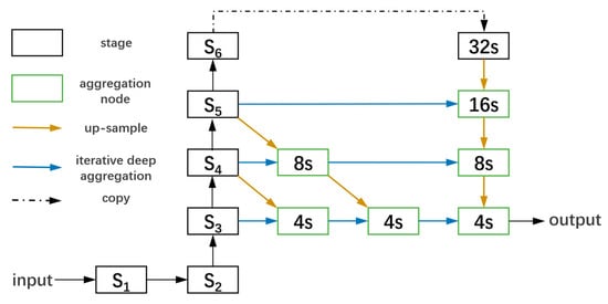
Figure 3.
The full convolution DLA-34 we use. Stages 3–6 are used to go through a further level of iterative deep aggregation. IDA for interpolation is used to project and up-sample nodes by 3 × 3 convolution while other nodes use 1 × 1 convolution.
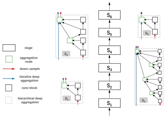
Figure 4.
IDA and HDA work together to fully extract features and fuse them well. A 7 × 7 convolution and a basic block form stage 1. Stage 2 is formed by a basic block. Other stages are combinations of bottleneck blocks and aggregation nodes [23].
2.1.2. Deformable Convolution
Deformable convolution in ConvNets v2 [26] is an optimized version of deformable convolution v1 [27]. It was designed to solve the biggest challenge in object recognition and detection, caused by geometric variations due to scale, pose, viewpoint, and part deformation. In DCNv1, augmented offsets are used to select deformed sampling locations so that the feature scale in convolution layers can be expanded. Nevertheless, the vision scale that DCNv1 produces is not precise enough to cover the area of interest, which is why DCNv2 was created. A learned offset and a learned feature amplitude ensure that DCNv2 has enhanced modeling power.
In this work, we replace convolution layers in up-sampling stages of DLA-34 with DCNv2 layers. They are also used in the recall-priority branch as skip connections to further integrate features.
2.2. Priority Branches
Our experiment results presented in Section 3.5 shows that the low recall rate is mainly caused by missed side-by-side ships and multi-scale ships, while the reduced precision rate is caused by ship-like objects. Although feature fusion in the backbone can improve these phenomena to some extent, the fundamental problems are not resolved. Therefore, we thought of splitting the ship detection task into two branches. Branches are designed to improve recall and precision separately. We use an anchor-free module to work as our recall-priority branch and an anchor-based module to act as the precision-priority branch.
2.2.1. Recall-Priority Branch
Experiment results presented in Section 3.5 show that the low recall rate of side-by-side ships can be attributed to the poor precision of produced center points. Frankly speaking, NMS, as used in previous methods, is just a remedy for the imprecise center points that detections predict. Moreover, the threshold of NMS is difficult to select; while a low threshold cannot effectively curb repeated boxes of the same object, close boxes that belong to different objects may be eliminated to get down to only one bounding box. Furthermore, this problem cannot be eradicated by other improved NMS methods, such as Soft-NMS.
If the center points produced by detections are precise enough, the detecting results will not need to be filtered by NMS. Because CenterNet provides a highly effective way to obtain precise center points, it can guarantee that objects closely abreast can be recalled without using NMS. We next use the feature maps from DLA-34 to produce a center-point map [26] instead of producing the coordinates of center points. C is the number of object types and R is the stride of output. In this paper, we set C to 1. According to Cao et al. [28] and Newell et al. [29], we set the default stride to R = 4, which means it will down-sample the output feature by a factor R. We resize the input image to 512 × 512, and after being processed by the branch, we obtain a heat map with the size of 128 × 128. At each location of output, five predicted parameters are produced: the key point , offset (, ), and size width () and height () of predicted bounding box [25]. means it is a center point of a detected ship, while corresponds to background. At the inference time, when such a feature map is remapped to the original image, it will create errors in accuracy. Therefore, an additional local offset is needed for each center point.
After obtaining the heat map, we extract the peaks of detected ships by finding the top 100 points whose value is greater than (or equal to) the eight neighboring points around it. This task can be performed by applying 3 × 3 max pooling to the heat map. If the center point in a 3 × 3 matrix equals to the 3 × 3 max pooling result of the matrix, it meets the requirement of being a peak point. The of the top 100 points is used to indicate the confidence in potential detecting ships. Meanwhile, the location of bounding boxes is produced by Equation (6) [25], where and are remapped coordinates from the low resolution of heat map to the original resolution.
During training, as proposed by Law et al. [30], we map each true ground center point to the resolution of the heat map by obtaining equivalent . Then, we use to label the down-sampled heat map by using a Gaussian kernel, presented in Equation (7) [30]. is a standard deviation related to the size of targets.
The loss function of this branch can be divided into three parts [25]: : focal loss [31] of heat map; : loss of offset; and : loss of object size. It is defined as
where and are scaling factors to confidence loss, offset loss, and size loss. and are hyperparameters [31] of confidence loss. We use N as the number of ships in an image. In this paper, , , , and [25].
2.2.2. Precision-Priority Branch
The detection results of the recall-priority branch in Section 3.5 show that the recall of side-by-side ships increases sharply, but the number of false alarms is high. This could be ascribed to mistaking ship-like floating objects on the water as ships. Meanwhile, despite the increased recall result, some ships of different sizes are still not detected. Therefore, the precision-priority branch has to make up for the false alarms and the missed ships recall-priority branch causes. Motivated by the output part of YOLOv3 [32], which draws on feature pyramid networks (FPNs) [33] and uses multiple scales to detect targets of different sizes, we use the anchor-based module to detect ships with multi-scale anchors, which can make up for the small ships missed by the recall-priority branch. To reduce the number of false alarms caused by another branch, a more powerful fusion architecture, BiFPN [34], is used to replace the feature pyramid in the YOLO module. We also use the K-means clustering method to obtain anchors based on the training boxes.
The main idea of the YOLO prediction module is to get three modules producing feature maps with different sizes after feature fusion. Using the output strides (32,16, 8) in YOLOv3 [32], we choose 16 × 16, 32 × 32, and 64 × 64 the sizes of the feature maps. For each feature map, three anchor priors are chosen. In order to select anchors based on the ship dataset, we apply the K-means algorithm to the annotated bounding boxes in the training dataset to obtain suitable priors [35]. In our dataset, the nine clusters are: (10, 14), (26, 22), (15, 49), (65, 30), (35, 59), (23, 149), (109, 74), (61, 151), and (143, 177). The first three clusters belong to module 1 (64 × 64), while the second and third three are the size of anchors belonging to modules 2 and 3, respectively.
For each location in an output feature map, the module produces three groups of data. Each group contains four coordinates () for each bounding box and its confidence value [32]. Therefore, the dimension of each module output is S × S × N, where S = 16, 32, 64; N = B × (5+C). In this paper, B, N= 3, 1.
As shown in Figure 5, and can be transformed to the coordinates of the center point relative to the upper left corner of the grid cells. and are parameters related to the width and height , of the bounding box priors. The predictions correspond to
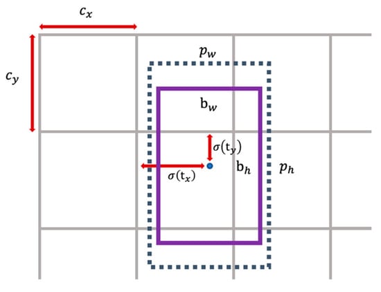
Figure 5.
To be the center location of predicted bounding box, and should go through sigmoid function , which will map the value of them to the range of 0 to 1. () stands for the offset to the upper left corner of the grid cells. () denotes the shape of anchor priors.
Following the method of YOLOv3, the loss of this branch is the sum of three parts [28]: loss of class (), loss of location (), and loss of confidence (). is based on sum of error loss, while and are realized with binary cross-entropy. The overall function is
where V in formulation (15) is a vector (), , P are confidence of bounding box and classification probability. The value of corresponds to whether the anchor box is responsible for the detected ship, while means the anchor box is out of business. and are scaling factors to weigh the loss. In this experiment, , and [32].
To decrease the number of false alarms in the detection results of recall-priority branch, we replace the feature pyramid in the YOLO module with BiFPN. This is a combination of efficient bidirectional cross-scale connections and weighted feature fusion [34]. Such connections are improved from PANet [36]. However, unlike PANet, nodes with only one input are removed. In addition, extra connections are added on each level from original input to output node, and each bidirectional path is treated as a feature layer in BiFPN. More high-level feature fusion is ensured by repeating the same layer multiple times. Fast normalized fusion is selected as weighted feature fusion, whose function is . In this function, , and is a value to keep stability. Such fusion is much more efficient than softmax-based fusion. The structure of precision-priority branch is shown in Figure 6.
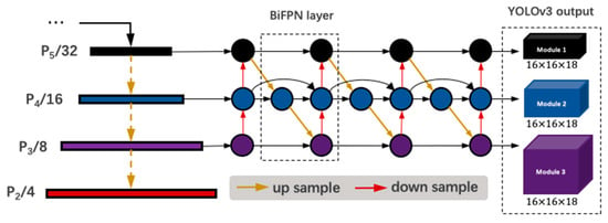
Figure 6.
The feature map produced by the backbone first go through BiFPN layers to integrate features further. Finally, the output modules from YOLOv3 give the predicted boxes based on anchor priors.
2.3. Priority-Based Selection
Priority-based selection serves as a filter to distinguish accurate boxes from the boxes from precision-priority branch () and the boxes from recall-priority branch ().
The strategy to filter boxes changes with whether they overlap:
- If has a high overlap with , we reserve .
- If a box has low or no overlap with all boxes from the other branch, and its confidence is higher than the threshold (the threshold is less strict for precision-priority branch), we reserve it.
Strategy (1) works in the area where and reach a consensus that ships exist, but they produce different boxes. At this time, is selected because the boxes from recall-priority can promise the recall for side-by-side ships. Strategy (2) deals with disagreements between the two branches. Boxes with low confidence are filtered and more boxes from the precision-priority branch are reserved because it is less likely to sound false alarms. Strategy (2) not only reduces the number of false alarms, but also keeps high potential boxes. This selection algorithm is shown in Figure 7.
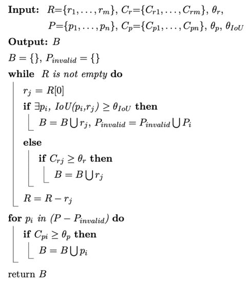
Figure 7.
and are the list of detection boxes produced by the two branches. and contain corresponding detection confidence. If boxes have overlap higher than , the box from the precision-priority branch will be eliminated. The confidence thresholds for the two branches are defined in the form of . The accuracy of detection results is the highest by setting , , and in our work.
PBS works as an efficient arbiter, ensuring high-quality boxes. The experiments described in the next section show that it leads to noticeable improvement compared with detection results from each branch.
3. Experiments and Results
To evaluate the performance of our proposed single-shot ship detection method, we compared it with other methods. The settings of the experiments introduced in this section include datasets, evaluation metrics, and compared methods. The efficiency of our method will also be presented.
3.1. Dataset
The HRSC2016 dataset contains images from two scenarios, including ships at sea and ships near the shore [24]. These 1061 images, including 2976 samples, were selected from Google Earth, and consist of images from six famous ports: Murmansk, Everett, Newport, Rhode Island, Mayport Naval Base, Norfolk Naval Base, and San Diego Naval Base. Their sizes range from 300 × 300 and 1500 × 900, while the resolutions vary from 2 m to 0.4 m. However, by studying the official images and annotations, the standard for annotations was found to be inconsistent. The two aspects to the problem are small ships and incomplete ships. In some images, they are annotated, but most are ignored by the author. Sample images and official annotated boxes are shown in Figure 8.
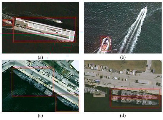
Figure 8.
Sample images and official annotated boxes. The inconsistent standards for small ships and incomplete ships are very noticeable.
To improve the dataset, we selected 360 more images from Google Earth to augment it and re-annotated these images. The resolutions of the images were between 0.27 m to 2.15 m. Their sizes range from 450 × 350 to 1200 × 850, and most of them are smaller than 1000 × 600. Like the original images in HRSC2016, most of the added samples are on the sea or near the shore. Sample images in our dataset are shown in Figure 9.
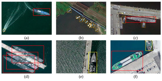
Figure 9.
Samples of augmented images and their new annotations based on levels. Red boxes represent large ships, orange boxes represent small ships, and yellow boxes represent incomplete ships.
We divided all the samples into large, small, and incomplete. Varying from the method of Lin et al. [37], we labeled complete ships with bounding box area larger than 96 × 96 pixels as large ships, and other complete ones as small ships. The improved dataset includes a total of 1421 images and 5058 samples, as shown in Table 1.

Table 1.
Number of samples in three sets
3.2. Evaluation Metrics
To measure the performance of our proposed methods quantitatively, we adopted precision, recall, and the precision–recall curve (PRC). The value of recall and precision can be calculated by TPs (true positives), FPs (false positives), and FNs (false negatives). If the IoU between a predicted box and ground truth is higher than 0.5, it is defined as TP. If the IoU is lower than 0.5, it is defined as FP. An actual object missed by detection is called an FN. Precision stands for the ratio of correct boxes and all predicted ones, and recall is the proportion of predicted correct boxes in all ground truth. AP, which is the area under PRC, is a comprehensive metric for avoiding the situation where recall and precision are unbalanced. The value of AP is between 0 and 1. The calculation methods are
3.3. Compared Methods
The detections we compare with consist of one-stage and two-stage frameworks. One-stage detections include YOLOv3 [32], RetinaNet [31], and FSAF [38]. Faster R-CNN [19] is the two-stage framework we use.
YOLOv3 is known for its efficiency. Referring to the feature pyramid structure and forming a multi-scale detection, it is good at detecting small objects. For better performance, we use darknet-53 with official pretrained weights as the backbone.
Using focal loss, RetinaNet is able to challenge the accuracy of two-stage detections after overcoming the problem of category imbalance. Images with a size of 640 × 640 go through ResNet-50 for feature extraction.
Like our proposed methods, FSAF also has an anchor-based branch and an anchor-free one. The best feature map is selected automatically by feature levels. Finally, predicted boxes produced by the two branches need to go through NMS. The base network of FSAF is also ResNet-50.
As a two-stage framework, Faster R-CNN applies a region proposal network to obtain candidate regions containing objects. The Fast R-CNN detector then classifies these regions. They share ResNet-50 as the backbone. Faster R-CNN is a popular method because of its high accuracy in detection tasks.
We adopted pretrained ResNet-50 on the Microsoft COCO dataset for RetinaNet, FSAF, and Faster R-CNN. For all methods, we used the Adam [39] optimization algorithm during 200 epochs of training. The initial learning rate remains 10−4 for the first 80 epochs and decays to 10−5 and 10−6 at epoch 80 and epoch 150. All networks are trained and tested in our dataset.
Considering that they all use NMS to merge results, networks with soft-NMS are also used.
3.4. Implementation Details
Data augmentation was applied before training the proposed network and the compared methods. It includes random flip respect to x-axis, shift augmentation, rescale 0.5, and rotate 90, 180, 270. In addition, more negative samples were added artificially to some images to improve the balance of positive and negative samples.
In the proposed single-shot detector, input images were resized to 512 × 512. Since NMS is not applied in the anchor-free recall-priority branch, boxes are selected if the confidence is higher than 0.3. The threshold of NMS in our anchor-based branch is 0.4. During training, the backbone is initialized by the weights of pretrained DLA-34 on the ImageNet database [40]. We follow Zhu et al. [38] to use as total optimization loss. The entire training process lasts for 200 epochs. The learning rate is set to 1.25 × 10⁻⁴ for the first 90 epochs and becomes 10 times smaller at epoch 90 and 150. The Adam optimizer is also used during the training. Our detector performs best after we trained it in this way. Our proposed method is implemented on the PyTorch framework and employs an Nvidia GeForce RTX 2080 Ti GPU with 11 GB memory for training.
3.5. Results
The comparison between our proposed network and other methods is presented both visually and quantitatively. The PRCs of five networks are shown in Figure 10, and the specific values of AP are compared in Table 2.
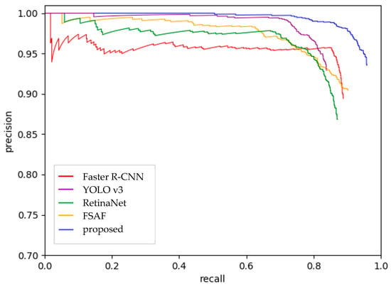
Figure 10.
PRC of different methods. The proposed network shows significant improvement in both precision and recall.
Table 2.
Recall, precision, and AP values of methods on the same dataset
From Figure 10, it is obvious that our method transcends all other networks in both precision and recall. Specifically, the recall is much higher than others. As a two-stage detector, Faster R-CNN achieves good results in recall because the region proposal network produces proper boxes for candidate ships. YOLOv3 has the best performance in precision but has the lowest recall of ships of the compared methods. By observing the visual outputs of YOLOv3, we find that some ships are selected by bounding boxes, but the size and location of boxes are not precise enough, thereby making recall the lowest. In contrast, the recall of RetinaNet is high but the precision is unsatisfactory. FSAF has the steadiest performance.
Table 2 shows that our method achieves the best AP value. In addition to its nearly 100% AP of large ships, it makes strong progress in detecting small ships and ships with incomplete forms. Among all compared networks, the AP of FSAF is closest to our performance, especially in detecting small ships. Using the same pretrained weights with Faster R-CNN and RetinaNet, we can speculate that the combination of anchor-free and anchor-based modules works well in the task of detecting ships. Compared with FSAF, the heat map method in our anchor-free module and the feature extraction architecture in the anchor-based module achieve 5.86%, 3.30%, 6.91%, and 25.19% performance gains in AP, APL, APS, and APIn respectively. The other three networks perform well in detecting large ships but are poor at detecting small ships and those with incomplete forms.
To further show the advantages of our proposed method, we list the number of false alarms and missed ships in Table 3. Surprisingly, YOLOv3 produces the same number of false alarms as the proposed network, despite the fact that it misses many more ships. At the early stages of our experiment, we found that YOLOv3 is good at accurate detection, so we used the YOLO output part as the main module in our precision-priority branch. From our observation of all the missed ships, we found that ships with different sizes were responsible for the most obstacles for improving recall value. By further fusing features, our method significantly reduced the number of obstacles. Meanwhile, our method was highly efficient in detecting side-by-side ships, reducing the number to zero, compared to tens of missed ships by other methods. Figure 11 shows the number of missed side-by-side ships after replacing NMS with soft-NMS in compared networks. Although soft-NMS is reported to significantly improve NMS [22], the number is only reduced by a small amount. Therefore, we believe that the key to solving this problem is to find center points more precisely instead of improving the performance of NMS. It is by this particular method that we can solve the problem so completely.
Table 3.
Number of missed ships and false alarms of methods
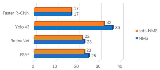
Figure 11.
Number of missed side-by-side ships. Soft-NMS improves a small degree when conducting this task.
The good performance of our detection method in both precision and recall can be attributed to PBS combining outputs from two branches. Table 4 clearly shows that the recall-priority branch is good at getting high recall while the other branch produces bounding boxes much more accurately. Because of PBS, the recall rises little compared to the recall-priority branch and the precision of the filtered results nearly reaches that of the precision-priority branch. It is easy to explain why the recall gets higher: more boxes mean more chances to hit the targets. Since we keep some results from the recall-priority branch, it is inevitable that more false alarms will occur and produce a lower precision. To attain higher precision, a recall-priority branch with better precision is needed. This is one of the goals of our future work.
Table 4.
Change of recall and precision after being filtered by PBS
Qualitative comparisons to other methods are shown in Figure 12. Compared with other methods, our networks achieve more robust detection of ship-like objects, side-by-side ships, and multi-scale ships. Our detector also shows favorable performance for incomplete ships.
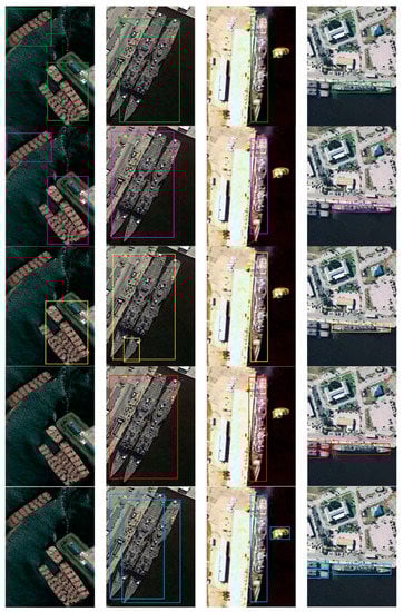
Figure 12.
Visual comparisons of detection results in different methods. From top to bottom, each row is Faster R-CNN, YOLOv3, RetinaNet, FSAF, and the proposed method, respectively.
The final efficiency analysis of networks is shown in Table 5. The inference speed of the proposed method is second only to YOLOv3. Considering that it is much better in precision and recall values, ranking second in speed is acceptable.
Table 5.
Average inference time of all methods
4. Conclusions
In this paper, we find that many of the obstacles of ship detection are caused by side-by-side ships, shape-like objects, and multi-scale ships. First, to reduce the number of false alarms and missed ships, we split the task into two branches: the recall-priority branch without NMS, which improves recall; and the precision-priority branch, which is good at detecting ships precisely. The final bounding boxes are selected from the results of two branches by PBS. Next, we constructed a dataset based on HRSC2016 with more samples and stricter annotation standards.
Through experiments on our dataset, we can make three conclusions. (1) The bottle neck to reducing the number of times side-by-side ships were missed is not the quality of the suppression algorithm, but the accuracy of detected center points of ships. Accordingly, the recall-priority branch improves recall to a high level. In addition, false alarms can be avoided to an extent by better fusion of features in our precision-priority branch. (2) Through the use of PBS, the combination of different branches works well, and the AP values increase sharply compared to other networks. (3) The inference time of our proposed method is short enough to meet the requirements of real-time detection (above 30 fps). In the future, we aim to simplify the network and put it on an ASIC chip.
Author Contributions
Conceptualization, Q.W.; Methodology, Y.Z.; Dataset, W.S. and J.J.; Software, Y.Z.; Validation, Q.W. and N.J.; Formal Analysis, J.J. and W.S.; Writing—Original Draft Preparation, Y.Z.; Writing—Review and Editing, N.J. and Q.W.; Supervision, Z.M.; Funding acquisition, Z.M. All authors have read and agreed to the published version of the manuscript.
Funding
This research was funded by National Natural Science Foundation of China (61176037).
Acknowledgments
The authors sincerely thank Dong G. C. and Shen F. Y. for their suggestions. The authors also want to thank You Y.L. and LetPub for their language polish of the writing.
Conflicts of Interest
The authors declare no conflict of interest.
References
- Li, Y.; Martinis, S.; Wieland, M. Urban flood mapping with an active self-learning convolutional neural network based on TerraSAR-X intensity and interferometric coherence. ISPRS J. Photogramm. Remote Sens. 2019, 152, 178–191. [Google Scholar] [CrossRef]
- Sun, S.; Li, C.; Chee, P.W.; Paterson, A.H.; Jiang, Y.; Xu, R.; Shehzad, T. Three-dimensional photogrammetric mapping of cotton bolls in situ based on point cloud segmentation and clustering. ISPRS J. Photogramm. Remote Sens. 2020, 160, 195–207. [Google Scholar] [CrossRef]
- Dong, C.; Liu, J.; Xu, F. Ship detection in optical remote sensing images based on saliency and a rotation-invariant descriptor. Remote Sens. 2018, 10, 400. [Google Scholar] [CrossRef]
- Barnum, J. Ship detection with high-resolution HF skywave radar. IEEE J. Ocean. Eng. 1986, 11, 196–209. [Google Scholar] [CrossRef]
- Tian, Y.; Wang, C.; Zhang, H. Spaceborne SAR Ship Detection and its Application on Marine fisheries monitoring. Remote Technol. Appl. 2007, 22, 503–512. [Google Scholar]
- Novak, L.M.; Halversen, S.D.; Owirka, G.; Hiett, M. Effects of polarization and resolution on SAR ATR. IEEE Trans. Aerosp. Electron. Syst. 1997, 33, 102–116. [Google Scholar] [CrossRef]
- Vachon, P.W.; Adlakha, P.; Edel, H.; Henschel, M.; Ramsay, B.; Flett, D.; Thomas, S. Canadian progress toward marine and coastal applications of synthetic aperture radar. Johns Hopkins APL Tech. Digest. 2000, 21, 33–40. [Google Scholar]
- Kaplan, L.M. Improved SAR target detection via extended fractal features. IEEE Trans. Aerosp. Electron. Syst. 2001, 37, 436–451. [Google Scholar] [CrossRef]
- Copeland, A.C.; Ravichandran, G.; Trivedi, M.M. Localized Radon transform-based detection of ship wakes in SAR images. IEEE Trans. Geosci. Remote Sens. 1995, 33, 35–45. [Google Scholar] [CrossRef]
- Proia, N.; Pagé, V. Characterization of a Bayesian ship detection method in optical satellite images. IEEE Geosci. Remote Sens. Lett. 2009, 7, 226–230. [Google Scholar] [CrossRef]
- Shu, C.; Ding, X.; Fang, C. Histogram of the oriented gradient for face recognition. Tsinghua Sci. Technol. 2011, 16, 216–224. [Google Scholar] [CrossRef]
- Liu, G.; Zhang, Y.; Zheng, X.; Sun, X.; Fu, K.; Wang, H. A new method on inshore ship detection in high-resolution satellite images using shape and context information. IEEE Geosci. Remote. Sens. Lett. 2013, 11, 617–621. [Google Scholar] [CrossRef]
- Yu, Y.; Guan, H.; Li, D.; Gu, T.; Tang, E.; Li, A. Orientation guided anchoring for geospatial object detection from remote sensing imagery. ISPRS J. Photogramm. Remote. Sens. 2020, 160, 67–82. [Google Scholar] [CrossRef]
- Lin, H.; Shi, Z.; Zou, Z. Fully convolutional network with task partitioning for inshore ship detection in optical remote sensing images. IEEE Geosci. Remote. Sens. Lett. 2017, 14, 1665–1669. [Google Scholar] [CrossRef]
- Xie, X.; Li, B.; Wei, X. Ship Detection in Multispectral Satellite Images Under Complex Environment. Remote Sens. 2020, 12, 792. [Google Scholar] [CrossRef]
- Chen, Y.; Li, Y.; Wang, J.; Chen, W.; Zhang, X. Remote Sensing Image Ship Detection under Complex Sea Conditions Based on Deep Semantic Segmentation. Remote Sens. 2020, 12, 625. [Google Scholar] [CrossRef]
- Dechesne, C.; Lefèvre, S.; Vadaine, R.; Hajduch, G.; Fablet, R. Ship Identification and Characterization in Sentinel-1 SAR Images with Multi-Task Deep Learning. Remote Sens. 2019, 11, 2997. [Google Scholar] [CrossRef]
- Rostami, M.; Kolouri, S.; Eaton, E.; Kim, K. Deep Transfer Learning for Few-Shot SAR Image Classification. Remote Sens. 2019, 11, 1374. [Google Scholar] [CrossRef]
- Ren, S.; He, K.; Girshick, R.; Sun, J. Faster r-cnn: Towards real-time object detection with region proposal networks. IEEE Trans. Pattern Anal. Mach. Intell. 2017, 39, 1137–1149. [Google Scholar] [CrossRef]
- Zhang, S.; Wu, R.; Xu, K.; Wang, J.; Sun, W. R-CNN-based ship detection from high resolution remote sensing imagery. Remote Sens. 2019, 11, 631. [Google Scholar] [CrossRef]
- Zhang, Z.; Guo, W.; Zhu, S.; Yu, W. Toward arbitrary-oriented ship detection with rotated region proposal and discrimination networks. IEEE Geosci. Remote Sens. Lett. 2018, 15, 1745–1749. [Google Scholar] [CrossRef]
- Bodla, N.; Singh, B.; Chellappa, R.; Davis, L.S. Soft-NMS--improving object detection with one line of code. In Proceedings of the 2017 IEEE International Conference on Computer Vision, Venice, Italy, 22–29 October 2017; pp. 5561–5569. [Google Scholar]
- Yu, F.; Wang, D.; Shelhamer, E.; Darrell, T. Deep layer aggregation. In Proceedings of the 2018 IEEE Conference on Computer Vision and Pattern Recognition, Salt Lake City, UT, USA, 18–23 June 2018; pp. 2403–2412. [Google Scholar]
- LB, W. A high resolution optical satellite image dataset for ship recognition and some new baselines. In Proceedings of the 6th International Conference on Pattern Recognition Applications and Methods, Porto, Portugal, 24–26 February 2017. [Google Scholar]
- Zhou, X.; Wang, D.; Krähenbühl, P. Objects as Points. arXiv 2019, arXiv:1904.07850. [Google Scholar]
- Zhu, X.; Hu, H.; Lin, S.; Dai, J. Deformable convnets v2: More deformable, better results. In Proceedings of the 2019 IEEE Conference on Computer Vision and Pattern Recognition, Long Beach, CA, USA, 15–20 June 2019; pp. 9308–9316. [Google Scholar]
- Dai, J.; Qi, H.; Xiong, Y.; Li, Y.; Zhang, G.; Hu, H.; Wei, Y. Deformable convolutional networks. In Proceedings of the 2017 IEEE International Conference on Computer Vision, Venice, Italy, 22–29 October 2017; pp. 764–773. [Google Scholar]
- Cao, Z.; Simon, T.; Wei, S.E.; Sheikh, Y. Realtime multi-person 2d pose estimation using part affinity fields. In Proceedings of the 2017 IEEE Conference on Computer Vision and Pattern Recognition, Honolulu, HI, USA, 21–26 July 2017; pp. 7291–7299. [Google Scholar]
- Newell, A.; Yang, K.; Deng, J. Stacked hourglass networks for human pose estimation. In Proceedings of the 2016 European Conference on Computer Vision, Amsterdam, The Netherlands, 8–16 October 2016; pp. 483–499. [Google Scholar]
- Law, H.; Deng, J. Cornernet: Detecting objects as paired keypoints. In Proceedings of the 2018 European Conference on Computer Vision, Munich, Germany, 8–14 September 2018; pp. 734–750. [Google Scholar]
- Lin, T.Y.; Goyal, P.; Girshick, R.; He, K.; Dollár, P. Focal loss for dense object detection. In Proceedings of the 2017 IEEE International Conference on Computer Vision, Venice, Italy, 22–29 October 2017; pp. 2980–2988. [Google Scholar]
- Redmon, J.; Farhadi, A. Yolov3: An Incremental Improvement. arXiv 2018, arXiv:1804.02767. [Google Scholar]
- Lin, T.Y.; Dollár, P.; Girshick, R.; He, K.; Hariharan, B.; Belongie, S. Feature pyramid networks for object detection. In Proceedings of the 2017 IEEE Conference on Computer Vision and Pattern Recognition, Honolulu, HI, USA, 21–26 July 2017; pp. 2117–2125. [Google Scholar]
- Tan, M.; Pang, R.; Le, Q.V. Efficientdet: Scalable and Efficient Object Detection. arXiv 2019, arXiv:1911.09070. [Google Scholar]
- Zhuang, S.; Wang, P.; Jiang, B.; Wang, G.; Wang, C. A Single Shot Framework with Multi-Scale Feature Fusion for Geospatial Object Detection. Remote Sens. 2019, 11, 594. [Google Scholar] [CrossRef]
- Liu, S.; Qi, L.; Qin, H.; Shi, J.; Jia, J. Path aggregation network for instance segmentation. In Proceedings of the 2018 IEEE Conference on Computer Vision and Pattern Recognition, Salt Lake City, UT, USA, 18–23 June 2018; pp. 8759–8768. [Google Scholar]
- Lin, T.Y.; Maire, M.; Belongie, S.; Hays, J.; Perona, P.; Ramanan, D.; Zitnick, C.L. Microsoft coco: Common objects in context. In Proceedings of the 2014 European Conference on Computer Vision, Zurich, Switzerland, 6–12 September 2014; pp. 740–755. [Google Scholar]
- Zhu, C.; He, Y.; Savvides, M. Feature selective anchor-free module for single-shot object detection. In Proceedings of the 2019 IEEE Conference on Computer Vision and Pattern Recognition, Long Beach, CA, USA, 15–20 June 2019; pp. 840–849. [Google Scholar]
- Kingma, D.P.; Ba, J. Adam: A Method for Stochastic Optimization. arXiv 2014, arXiv:1412.6980. [Google Scholar]
- Deng, J.; Dong, W.; Socher, R.; Li, L.J.; Li, K.; Fei-Fei, L. Imagenet: A large-scale hierarchical image database. In Proceedings of the 2009 IEEE Conference on Computer Vision and Pattern Recognition, Miami Beach, FL, USA, 20–25 June 2009; pp. 248–255. [Google Scholar]


© 2020 by the authors. Licensee MDPI, Basel, Switzerland. This article is an open access article distributed under the terms and conditions of the Creative Commons Attribution (CC BY) license (http://creativecommons.org/licenses/by/4.0/).