Uncertainty in Measured Raindrop Size Distributions from Four Types of Collocated Instruments

 ,
,  and
and
Abstract
1. Introduction
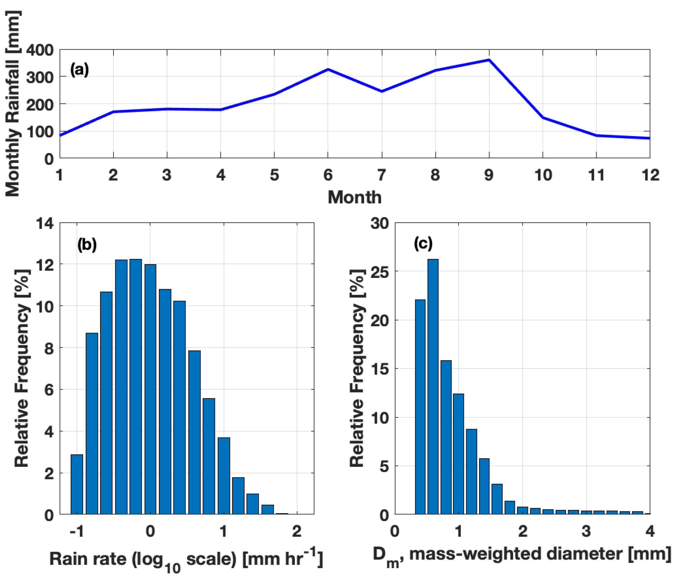
2. Data
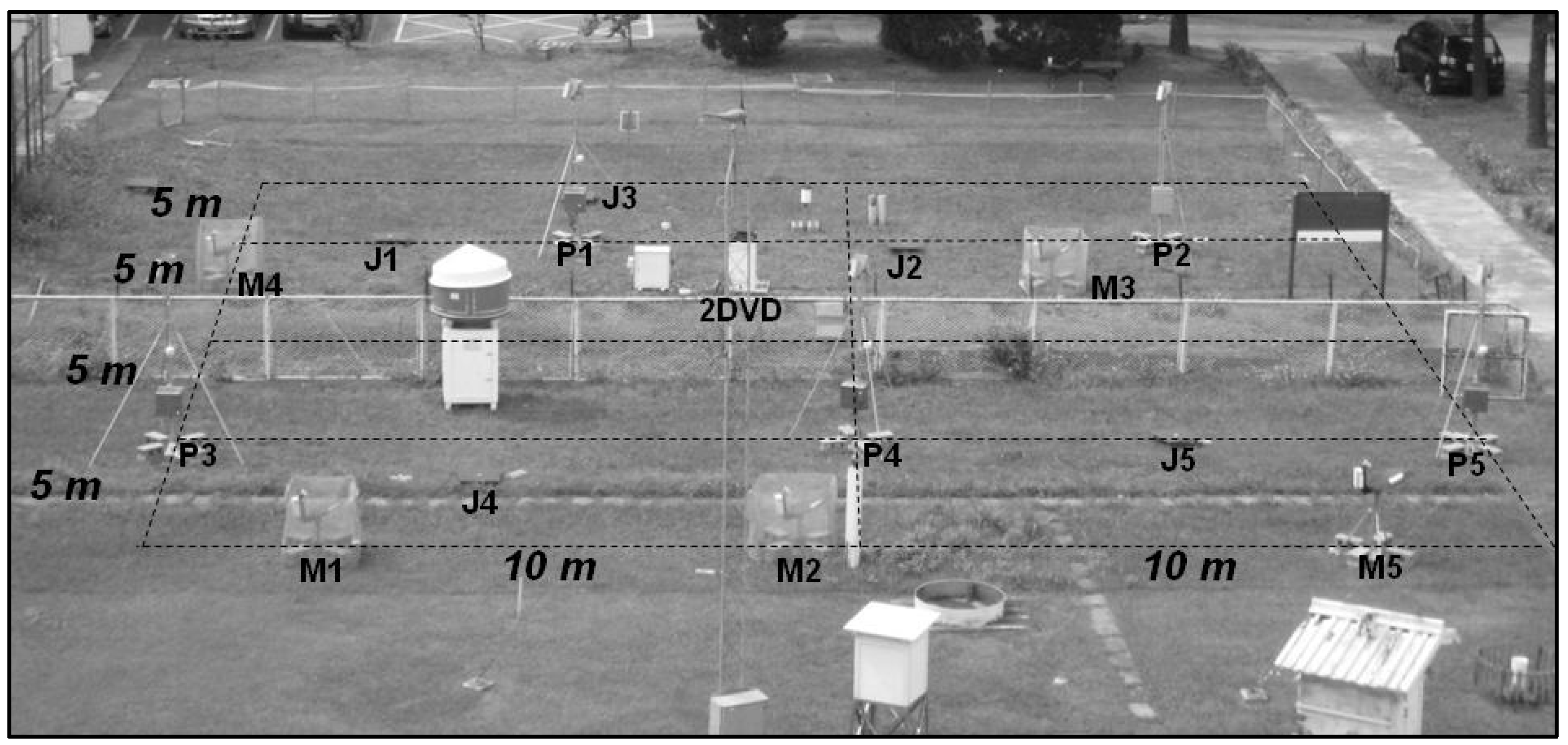
2.1. Instrumentations
2.2. Preprocessing of Disdrometer Data
3. Methodology of Estimating Measurement Bias and Uncertainty
3.1. Bias Estimation and Correction
3.2. Estimation of Measurement Noise
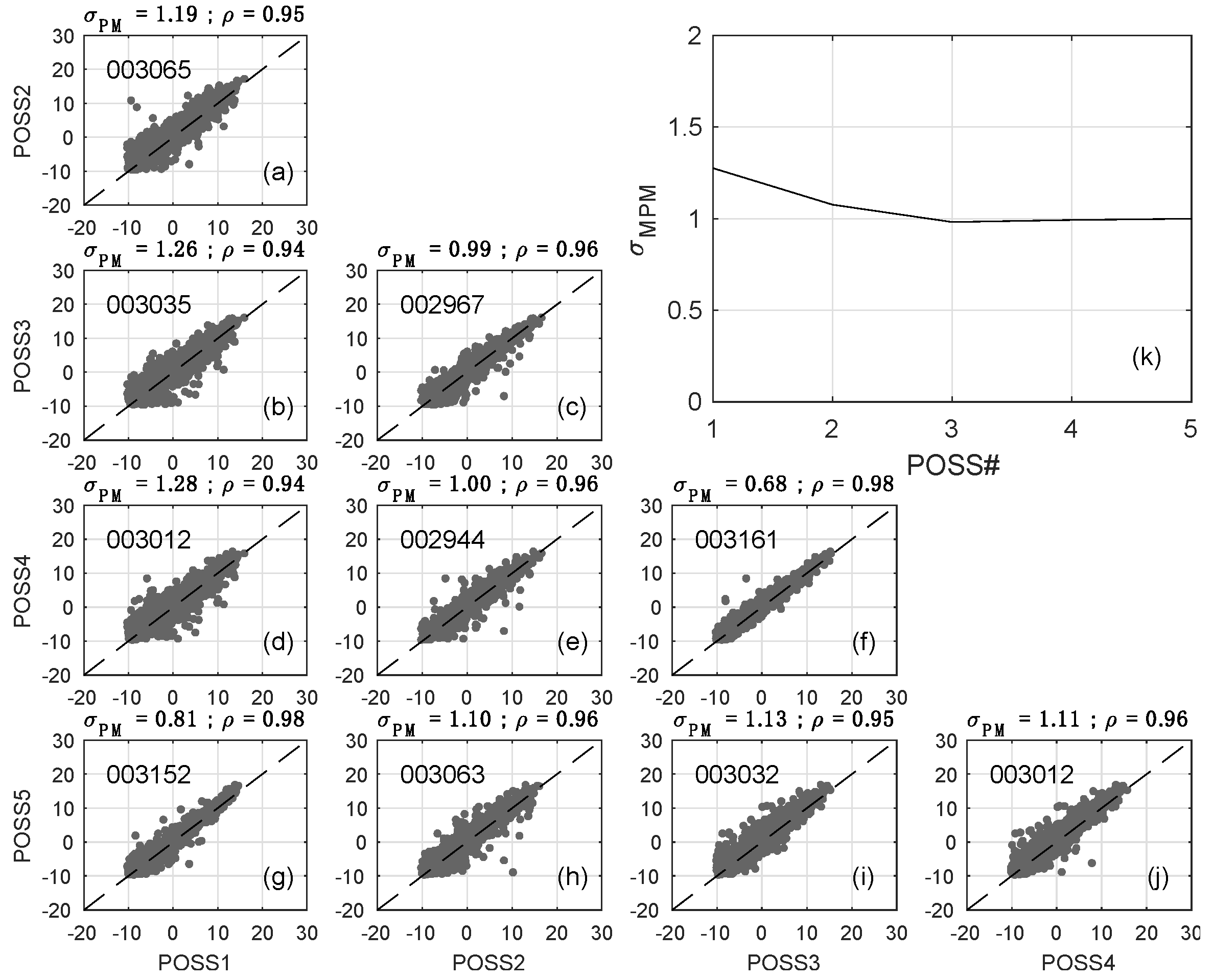
3.2.1. Standard Deviation of Measurement Noise Estimated from Paired Measurements ()
3.2.2. Standard Deviation of Measurement Noise Estimated from Multiple Paired Measurements ()
3.2.3. Standard Deviation of Measurement Noise from Paired Cross-Type Measurements ()
4. Results
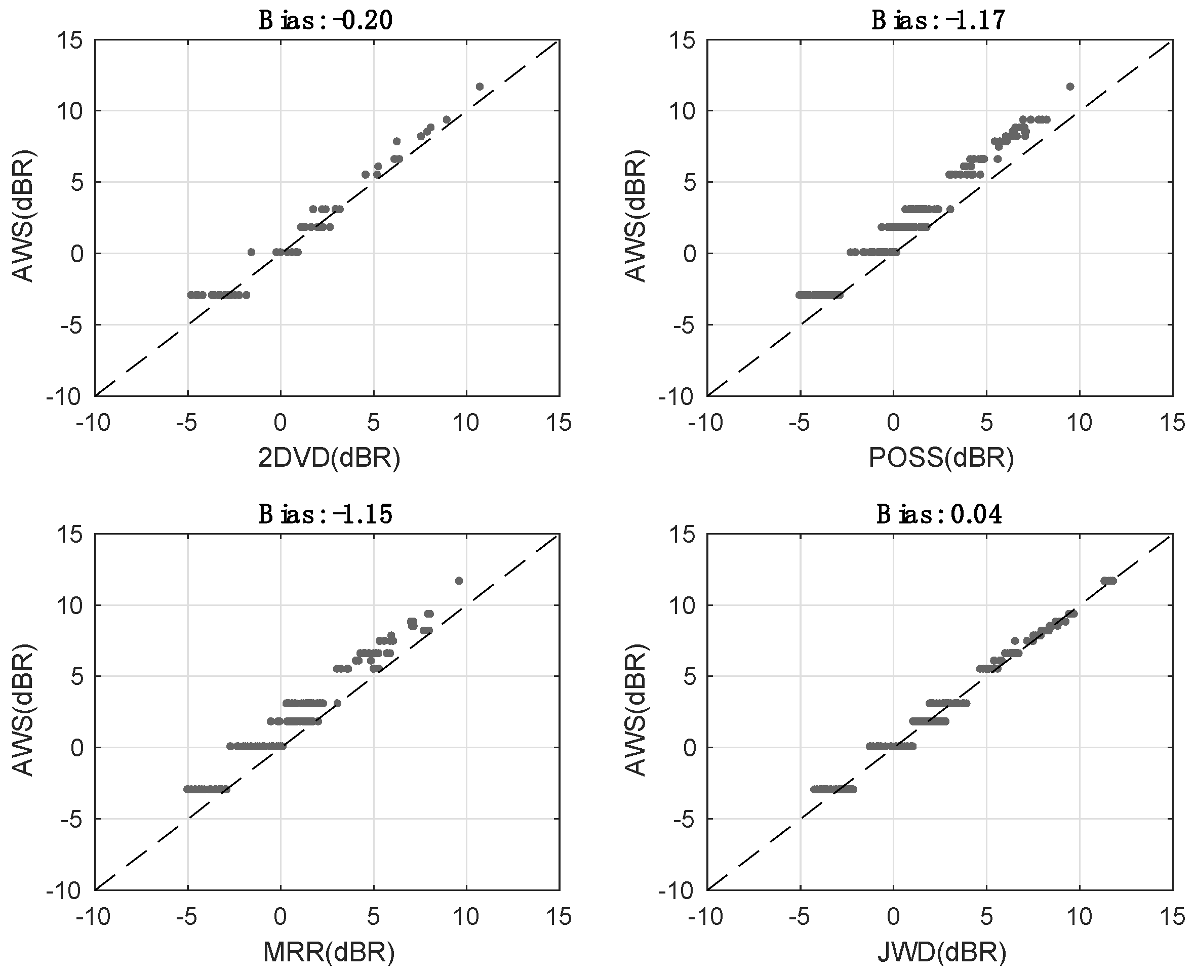
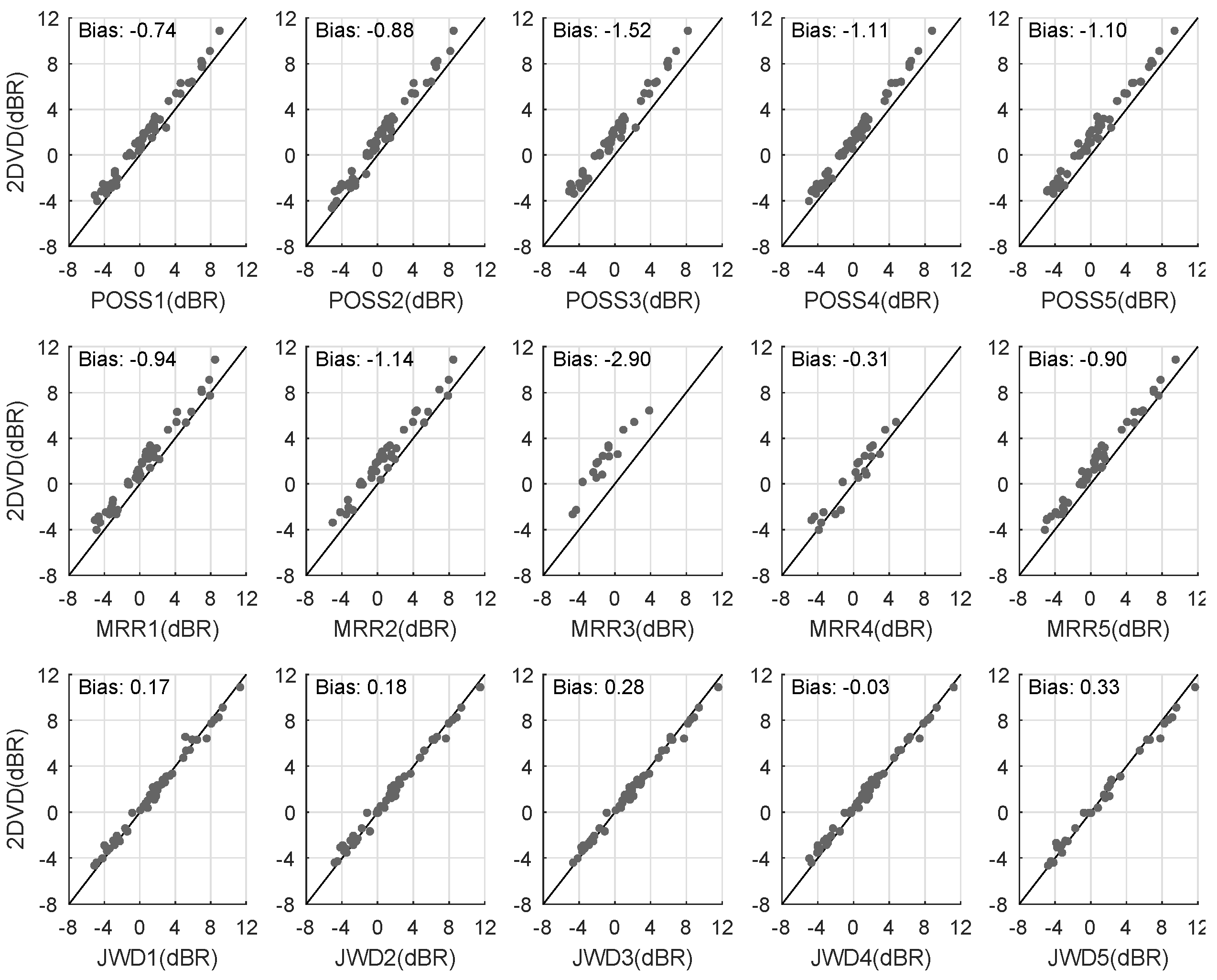
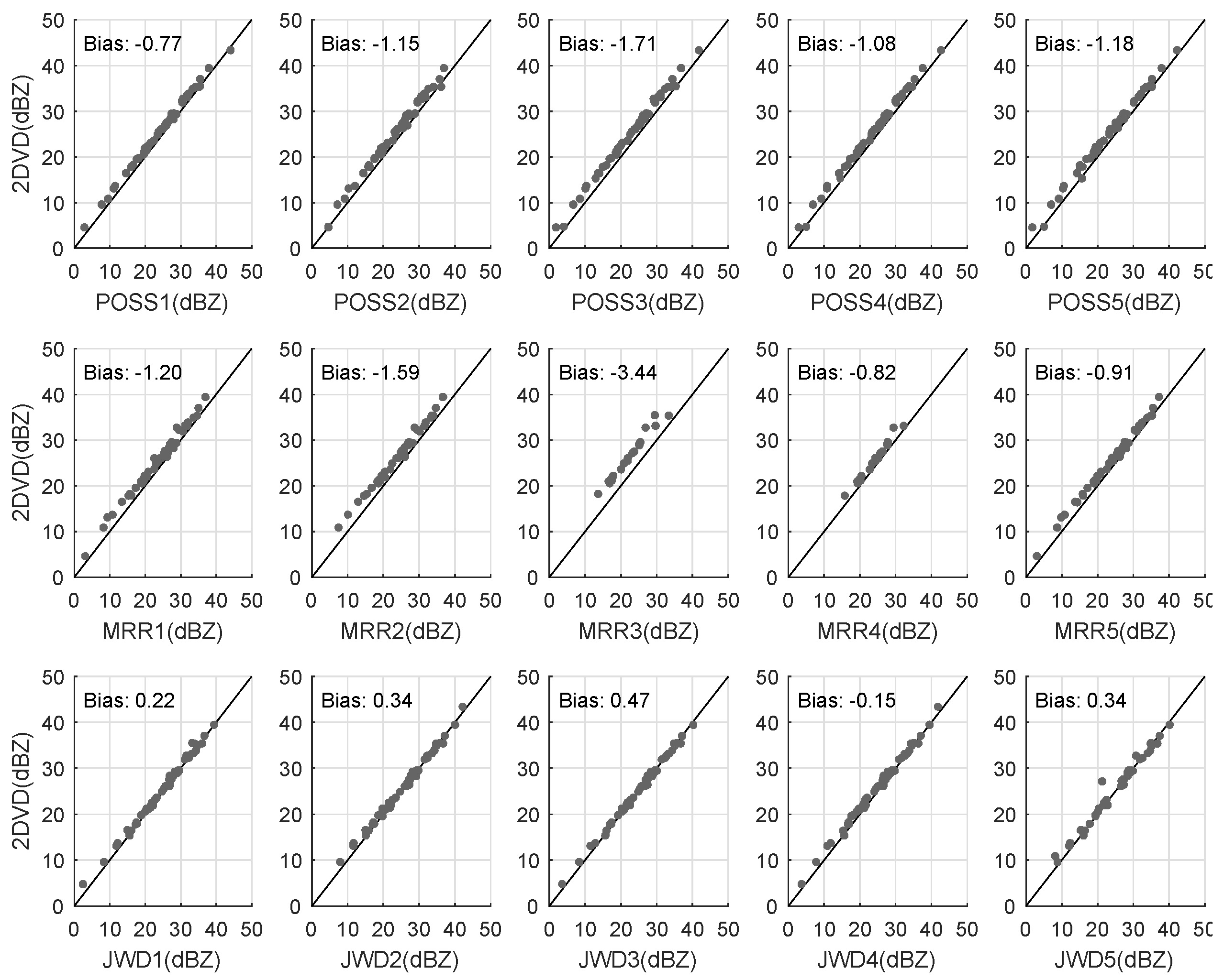
4.1. Measurement Bias of Individual Disdrometer
4.1.1. Comparison of R and Z
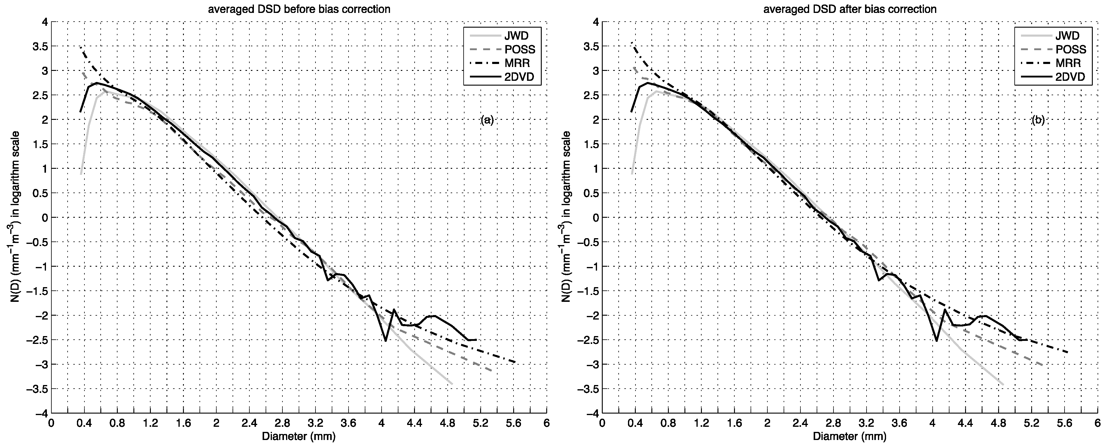
4.1.2. Averaged DSD
4.1.3. Bias Correction
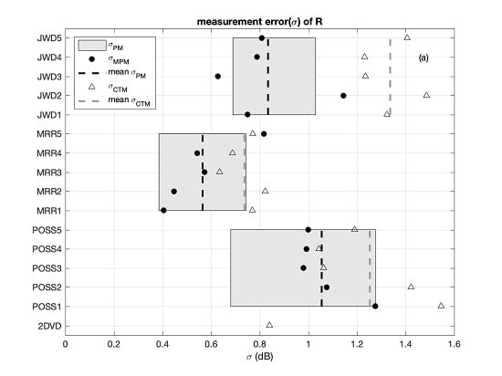
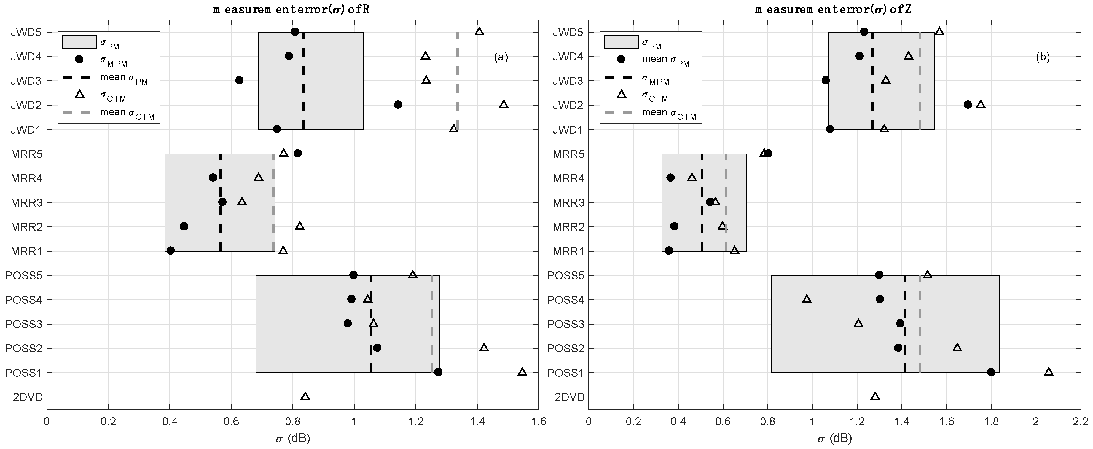
4.2. Measurement Uncertainty
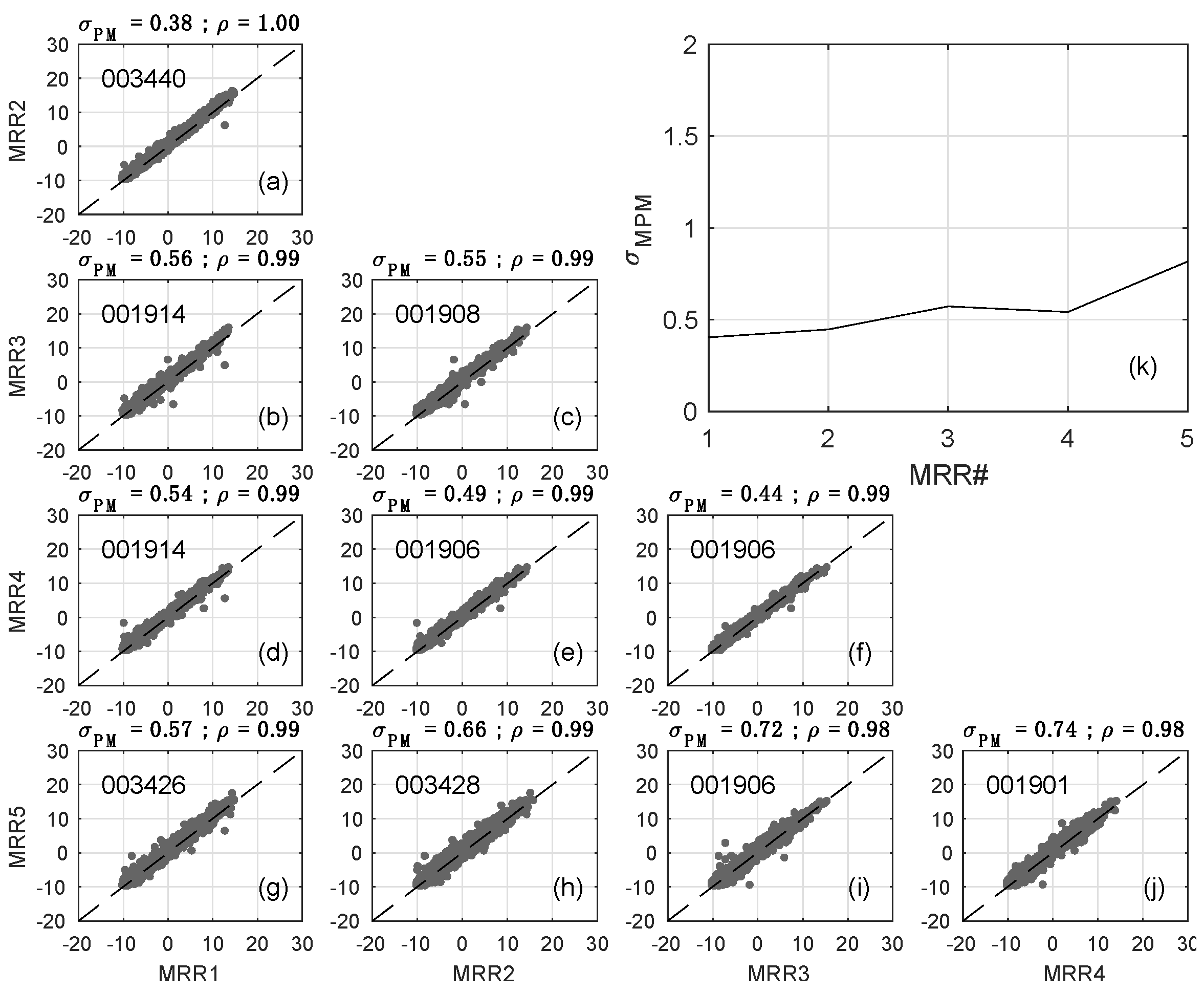
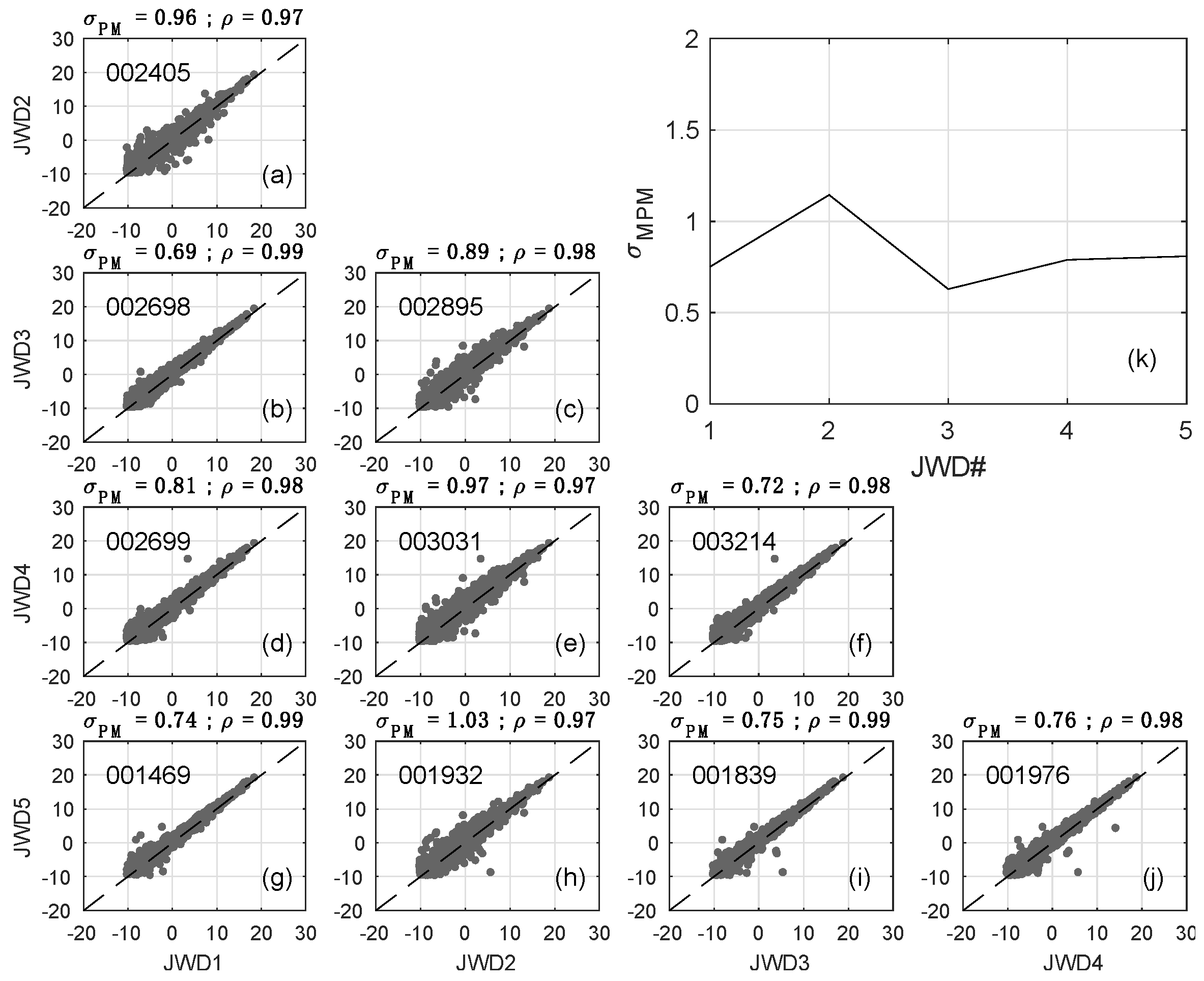
4.2.1. Measurement Uncertainties of R and Z from Paired Measurements () and Multiple Paired Measurements ()
4.2.2. Measurement Uncertainties of R and Z from Paired “Cross-Type” Disdrometer Measurements ()
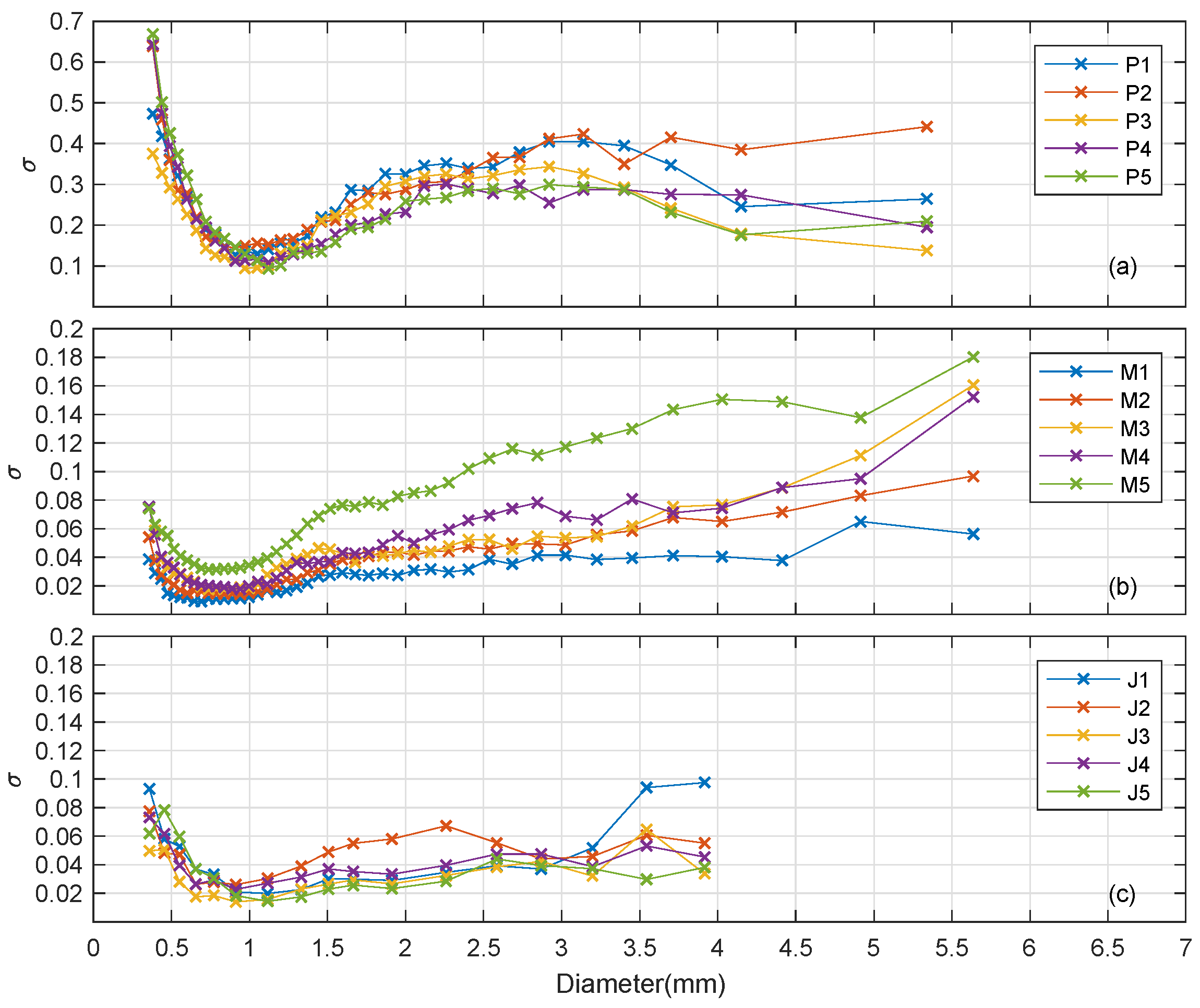
4.2.3. Measurement Errors of Raindrop Concentration (N(D))
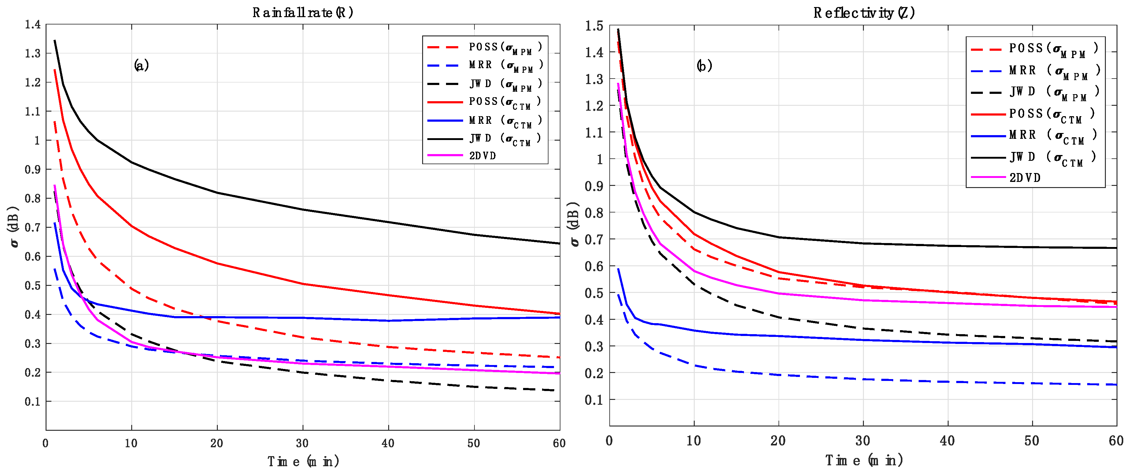
4.3. Measurement Uncertainty as a Function of Temporal Integration
5. Discussion
6. Conclusions
Author Contributions
Funding
Acknowledgments
Conflicts of Interest
References
- Lee, G.W. Sources of errors in rainfall measurements by polarimetric radar: Variability of drop size distributions, observational noise, and variation of relationships between R and polarimetric parameters. J. Atmos. Ocean. Technol. 2006, 23, 1005–1028. [Google Scholar] [CrossRef]
- Chang, W.-Y.; Wang, T.-C.C.; Lin, P.-L. Characteristics of the raindrop size distribution and drop shape relation in typhoon systems in the western pacific from the 2D video disdrometer and NCU C-band polarimetric radar. J. Atmos. Ocean. Technol. 2009, 26, 1973–1993. [Google Scholar] [CrossRef]
- Tapiador, F.J.; Checa, R.; De Castro, M. An experiment to measure the spatial variability of rain drop size distribution using sixteen laser disdrometers. Geophys. Res. Lett. 2010. [Google Scholar] [CrossRef]
- Jaffrain, J.; Berne, A. Experimental quantification of the sampling uncertainty associated with measurements from PARSIVEL disdrometers. J. Hydrometeor. 2011, 12, 352–370. [Google Scholar] [CrossRef]
- Jaffrain, J.; Berne, A. Quantification of the small-scale spatial structure of the raindrop size distribution from a network of disdrometers. J. Appl. Meteorol. Climatol. 2012, 51, 941–953. [Google Scholar] [CrossRef]
- Jaffrain, J.; Studzinski, A.; Berne, A. A network of disdrometers to quantify the small-scale variability of the raindrop size distribution. Water Resour. Res. 2011, 47, W00H06. [Google Scholar] [CrossRef]
- Chang, W.Y.; Vivekanandan, J.; Ikeda, K.; Lin, P.L. Quantitative precipitation estimation of the epic 2013 Colorado flood event: Polarization radar-based variational scheme. J. Appl. Meteorol. Climatol. 2016, 55, 1477–1495. [Google Scholar] [CrossRef]
- Zawadzki, L. On radar–raingage comparison. J. Appl. Meteorol. 1975, 14, 1430–1436. [Google Scholar] [CrossRef]
- Bringi, V.N.; Chandrasekar, V. Polarimetric Doppler Weather Radar: Principles and Applications; Cambridge University Press: Cambridge, MA, USA, 2011; p. 636. [Google Scholar]
- Lee, G.W.; Zawadzki, L. Variability of drop size distributions: Time-scale dependence of the variability and its effects on rain estimation. J. Appl. Meteorol. 2005, 44, 241–255. [Google Scholar] [CrossRef]
- Bringi, V.N.; Chandrasekar, V.; Hubbert, J.; Gorgucci, E.; Randeu, W.Y.; Schoenhuber, M. Raindrop size distribution in different climatic regimes from disdrometer and dual-polarized radar analysis. J. Atmos. Sci. 2003, 60, 354–365. [Google Scholar] [CrossRef]
- Cao, Q.; Zhang, G.; Brandes, E.; Schuur, T.; Ryzhkov, A.; Ikeda, K. Analysis of video disdrometer and polarimetric radar data to characterize rain microphysics in oklahoma. J. Appl. Meteorol. Climatol. 2008, 47, 2238–2255. [Google Scholar] [CrossRef]
- Chang, W.Y.; Lee, W.C.; Liou, Y.C. The kinematic and microphysical characteristics and associated precipitation efficiency of subtropical convection during SoWMEX/TiMREX. Mon. Weather Rev. 2015, 143, 317–340. [Google Scholar] [CrossRef]
- Thurai, M.; Gatlin, P.; Bringi, V.N.; Petersen, W.; Kennedy, P.; Notaroš, B.; Carey, L. Toward completing the raindrop size spectrum: Case studies involving 2D-video disdrometer, droplet spectrometer, and polarimetric radar measurements. J. Appl. Meteorol. Clim. 2017, 56, 877–896. [Google Scholar] [CrossRef]
- Thompson, E.J.; Rutledge, S.A.; Dolan, B.; Thurai, M. Drop size distributions and radar observations of convective and stratiform rain over the equatorial indian and west pacific oceans. J. Atmos. Sci. 2015, 72, 4091–4125. [Google Scholar] [CrossRef]
- Raupach, T.H.; Berne, A. Small-scale variability of the raindrop size distribution and its effect on areal rainfall retrieval. J. Hydrometeor. 2016, 17, 2077–2104. [Google Scholar] [CrossRef]
- Lee, M.T.; Lin, P.L.; Chang, W.Y.; Seela, B.K.; Janapati, J. Microphysical characteristics and types of precipitation for different seasons over North Taiwan. J. Meteorol. Soc. Jpn. Ser. II 2019. [Google Scholar] [CrossRef]
- Larsen, M.L.; Teves, J.B. Identifying individual rain events with a dense disdrometer network. Adv. Meteorol. 2015. [Google Scholar] [CrossRef]
- Jameson, A.R.; Larsen, M.L. Estimates of the statistical two-dimensional spatial structure in rain over a small network of disdrometers. Meteorol. Atmos. Phys. 2016, 125, 401–413. [Google Scholar] [CrossRef]
- Tokay, A.; D’Adderio, L.P.; Wolff, D.B.; Petersen, W.A. A field study of pixel-scale variability of raindrop size distribution in the mid-Atlantic region. J. Hydrometeorol. 2016, 17, 1855–1868. [Google Scholar] [CrossRef]
- Tokay, A.; D’Adderio, L.P.; Porcù, F.; Wolff, D.B.; Petersen, W.A. A field study of footprint-scale variability of raindrop size distribution. J. Hydrometeorol. 2017, 18, 3165–3179. [Google Scholar] [CrossRef]
- Joss, J.; Waldvogel, A. Raindrop size distribution and sampling size errors. J. Atmos. Sci. 1969, 26, 566–569. [Google Scholar] [CrossRef]
- Lee, G.W.; Zawadzki, L. Variability of drop size distributions: Noise and noise filtering in disdrometric data. J. Appl. Meteorol. 2005, 44, 634–652. [Google Scholar] [CrossRef]
- Tokay, A.; Bashor, P.G.; Wolff, K.R. Error characteristics of rainfall measurements by collocated Joss–Waldvogel disdrometers. J. Atmos. Ocean. Technol. 2005, 22, 513–527. [Google Scholar] [CrossRef]
- Tokay, A.; Petersen, W.A.; Gatlin, P.; Wingo, M. Comparison of raindrop size distribution measurements by collocated disdrometers. J. Atmos. Ocean. Technol. 2013, 30, 1672–1690. [Google Scholar] [CrossRef]
- Miriovsky, B.J. An experimental study of small-scale variability of radar reflectivity using disdrometer observations. J. Appl. Meteorol. 2004, 43, 106–118. [Google Scholar] [CrossRef]
- Krajewski, W.F.; Kruger, A.; Caracciolo, C.; Golé, P.; Barthes, L.; Creutin, J.-D.; Vinson, J.-P. DEVEX-disdrometer evaluation experiment: Basic results and implications for hydrologic studies. Adv. Water Resour. 2006, 29, 311–325. [Google Scholar] [CrossRef]
- Schönhuber, M.; Urabn, H.E.; Poiares Baptista, J.P.V.; Randeu, W.L.; Riedler, W. Weather radar versus 2D-video-distrometer data. In Weather Radar Technology for Water Resources Management; Braga, B., Jr., Massambani, O., Eds.; UNESCO: Paris, France, 1997; pp. 159–171. [Google Scholar]
- Löffler-Mang, M.; Joss, J. An optical disdrometer for measuring size and velocity of hydrometeors. J. Atmos. Ocean. Technol. 2000, 17, 130–139. [Google Scholar] [CrossRef]
- Tokay, A.; Kruger, A.; Krajewski, W.F. Comparison of drop size distribution measurements by impact and optical disdrometers. J. Appl. Meteorol. 2001, 40, 2083–2097. [Google Scholar] [CrossRef]
- Sheppard, B.E.; Joe, P.I. Comparison of raindrop size distribution measurements by a Joss–Waldvogel disdrometer, a PMS 2DG spectrometer, and a POSS Doppler radar. J. Atmos. Ocean. Technol. 1994, 11, 874–887. [Google Scholar] [CrossRef]
- Sheppard, B.E. Measurement of raindrop size distribution using a small Doppler radar. J. Atmos. Ocean. Technol. 1990, 7, 255–268. [Google Scholar] [CrossRef]
- Jou, B.J.-D.; Lee, W.-C.; Johnson, R.H. An overview of SoWMEX/TiMREX and its operation. In The Global Monsoon System: Research and Forecast, 2nd ed.; Chang, C.-P., Ed.; World Scientific: Singapore, 2011; pp. 303–318. [Google Scholar]
- Chen, C.S.; Chen, Y.L. The rainfall characteristics of Taiwan. Mon. Weather Rev. 2003, 131, 1323–1341. [Google Scholar] [CrossRef]
- Campos, E.; Zawadzki, L. Instrumental uncertainties in Z–R relations. J. Appl. Meteorol. 2000, 39, 1088–1102. [Google Scholar] [CrossRef]
- Löffler-Mang, M.; Kunz, M.; Schmid, W. On the performance of a low-cost K-band Doppler radar for quantitative rain measurement. J. Atmos. Ocean. Technol. 1999, 16, 379–387. [Google Scholar] [CrossRef]
- Atlas, D.; Srivastava, R.C.; Sekhon, R.S. Doppler radar characteristics of precipitation at vertical incidence. Rev. Geophys. 1973, 11, 1–35. [Google Scholar] [CrossRef]
- Gunn, R.; Kinzer, G.D. The terminal velocity of fall for water droplets in stagnant air. J. Atmos. Sci. 1949, 6, 243–248. [Google Scholar] [CrossRef]
- Sheppard, B.E. Effect of irregularities in the diameter classification of raindrop by Joss–Waldvogel disdrometer. J. Atmos. Ocean. Technol. 1990, 7, 180–183. [Google Scholar] [CrossRef]
- Barthazy, E.J.; Göke, S.; Schefold, R.; Högl, D. An optical array instrument for shape and fall velocity measurements of hydrometeors. J. Atmos. Ocean. Technol. 2004, 21, 1400–1416. [Google Scholar] [CrossRef]
- Nešpor, V.; Krajewski, W.F.; Kruger, A. Wind-induced error of raindrop size distribution measurement using a two-dimensional video disdrometer. J. Atmos. Ocean. Technol. 2000, 17, 1483–1492. [Google Scholar] [CrossRef]
- Kruger, A.; Krajewski, W.F. Two-dimensional video disdrometer: A description. J. Atmos. Ocean. Technol. 2002, 19, 602–617. [Google Scholar] [CrossRef]
- Brandes, E.A.; Zhang, G.; Vivekanandan, J. Experiments in rainfall estimation with a polarimetric radar in a subtropical environment. J. Appl. Meteorol. 2002, 41, 674–685. [Google Scholar] [CrossRef]
- Thurai, M.; Bringi, V.N. Drop axis ratios from 2D video disdrometer. J. Atmos. Ocean. Technol. 2005, 22, 966–978. [Google Scholar] [CrossRef]
- Williams, C.R.; Kruger, A.; Gage, K.S.; Tokay, A.; Cifelli, R.; Krajewski, W.F.; Kummerow, C. Comparison of simultaneous rain drop size distributions estimated from two surface disdrometers and a UHF profiler. Geophys. Res. Lett. 2000, 27, 1763–1766. [Google Scholar] [CrossRef]
- Tokay, A.; Kruger, A.; Krajewski, W.F.; Kucera, P.A.; Filho, A.J.P. Measurements of drop size distribution in the southwestern Amazon basin. J. Geophys. Res. 2002, 107, 8052. [Google Scholar] [CrossRef]
- Ciach, G.J. Local random errors in tipping-bucket rain gauge measurements. J. Atmos. Ocean. Technol. 2003, 20, 752–759. [Google Scholar] [CrossRef]
- Maahn, M.; Kollias, P. Improved micro rain radar snow measurements using Doppler spectra post-processing. Atmos. Meas. Tech. Discuss. 2012, 5, 4771–4808. [Google Scholar] [CrossRef]
- Chandrasekar, V.; Gori, E.G. Multiple disdrometer observations of rainfall. J. Appl. Meteorol. 1991, 30, 1514–1520. [Google Scholar] [CrossRef][Green Version]
- Gage, K.S.; Clark, W.L.; Williams, C.R.; Tokay, A. Determining reflectivity measurement error from serial measurements using paired disdrometers and profilers. Geophys. Res. Lett. 2004, 31, L23107. [Google Scholar] [CrossRef]
- Berne, A.; Uijlenhoet, R. Quantification of the radar reflectivity sampling error in non-stationary rain using paired disdrometers. Geophys. Res. Lett. 2005, 32, L19813. [Google Scholar] [CrossRef]
- Tokay, A.; Wolff, D.B.; Petersen, W.A. Evaluation of the new version of the laser-optical disdrometer, OTT Parsivel2. J. Atmos. Ocean. Technol. 2014, 31, 1276–1288. [Google Scholar] [CrossRef]
- Tapiador, F.J.; Navarro, A.; Moreno, R.; Jiménez-Alcázar, A.; Marcos, C.; Tokay, A.; Durán, L.; Bodoque, J.M.; Martín, R.; Petersen, W.; et al. On the optimal measuring area for pointwise rainfall estimation: A dedicated experiment with 14 laser disdrometers. J. Hydrometeorol. 2017, 18, 753–760. [Google Scholar] [CrossRef]
- Joss, J.; Gori, E.G. Shapes of raindrop size distribution. J. Appl. Meteorol. 1978, 17, 1054–1061. [Google Scholar] [CrossRef]


| ID | Type (Affiliation, Code Name) | Rainy Minutes | Time Lag (min) | Correlation Coefficient after Applying Time Lag (before Applying Time Lag) |
|---|---|---|---|---|
| 0 | 2DVD (NCU, 2DVD) | 2985 | - | |
| 1 | POSS (McGill, P1) | 3624 | 1 | 0.961(0.939) |
| 2 | POSS (PKNU, P2) | 3128 | 1 | 0.949(0.898) |
| 3 | POSS (ECCC, P3) | 3241 | 0 | 0.958 |
| 4 | POSS (ECCC, P4) | 3217 | 0 | 0.957 |
| 5 | POSS (ECCC, P5) | 3213 | 1 | 0.969(0.915) |
| 6 | MRR (CCU, M1) | 3499 | 1 | 0.957(0.886) |
| 7 | MRR (CCU, M2) | 3501 | 1 | 0.959(0.883) |
| 8 | MRR (CCU, M3) | 1949 | 1 | 0.948(0.847) |
| 9 | MRR (CCU, M4) | 1943 | 1 | 0.923(0.862) |
| 10 | MRR (KNU, M5) | 3496 | 1 | 0.961(0.898) |
| 11 | JWD (NCU, J1) | 2762 | 0 | 0.969 |
| 12 | JWD (CCU, J2) | 3098 | 0 | 0.958 |
| 13 | JWD (NCU, J3) | 3288 | 0 | 0.968 |
| 14 | JWD (NCU, J4) | 3457 | 0 | 0.965 |
| 15 | JWD (NCU, J5) | 2019 | 0 | 0.967 |
| Channel, i | Di (mm) | νi (m s−1) | Vi (m3 s−1) | Channel, i | Di (mm) | νi (m s−1) | Vi (m3 s−1) | ||
|---|---|---|---|---|---|---|---|---|---|
| 1 | 0.34 | 0.05 | 1.350 | 0.32 | 18 | 1.46 | 0.09 | 5.314 | 0.11 × 10² |
| 2 | 0.38 | 0.05 | 1.530 | 0.44 | 19 | 1.55 | 0.10 | 5.530 | 0.11 × 10² |
| 3 | 0.44 | 0.05 | 1.796 | 0.71 | 20 | 1.65 | 0.10 | 5.760 | 0.15 × 10² |
| 4 | 0.49 | 0.05 | 2.016 | 0.78 | 21 | 1.76 | 0.11 | 6.002 | 0.18 × 10² |
| 5 | 0.54 | 0.06 | 2.224 | 0.10 × 101 | 22 | 1.87 | 0.12 | 6.230 | 0.21 × 10² |
| 6 | 0.60 | 0.06 | 2.470 | 0.13 × 101 | 23 | 2.00 | 0.12 | 6.490 | 0.26 × 10² |
| 7 | 0.66 | 0.06 | 2.710 | 0.19 × 101 | 24 | 2.12 | 0.13 | 6.736 | 0.30 × 10² |
| 8 | 0.72 | 0.06 | 2.950 | 0.24 × 101 | 25 | 2.26 | 0.14 | 7.011 | 0.36 × 10² |
| 9 | 0.78 | 0.06 | 3.190 | 0.29 × 101 | 26 | 2.40 | 0.15 | 7.270 | 0.41 × 10² |
| 10 | 0.84 | 0.06 | 3.430 | 0.37 × 101 | 27 | 2.56 | 0.17 | 7.510 | 0.49 × 10² |
| 11 | 0.91 | 0.07 | 3.706 | 0.43 × 101 | 28 | 2.73 | 0.18 | 7.765 | 0.58 × 10² |
| 12 | 0.97 | 0.07 | 3.922 | 0.52 × 101 | 29 | 2.92 | 0.20 | 7.964 | 0.73 × 10² |
| 13 | 1.05 | 0.07 | 4.183 | 0.58 × 101 | 30 | 3.14 | 0.23 | 8.200 | 0.92 × 10² |
| 14 | 1.12 | 0.08 | 4.396 | 0.69 × 101 | 31 | 3.40 | 0.28 | 8.440 | 0.11 × 10³ |
| 15 | 1.20 | 0.08 | 4.640 | 0.79 × 101 | 32 | 3.70 | 0.36 | 8.660 | 0.11 × 10³ |
| 16 | 1.28 | 0.08 | 4.852 | 0.86 × 101 | 33 | 4.15 | 0.56 | 8.898 | 0.15 × 10³ |
| 17 | 1.37 | 0.09 | 5.091 | 0.10 × 10² | 34 | 5.34 | 1.84 | 9.134 | 0.19 × 10³ |
| Channel, i | Di (mm) | (mm) | νi (m s−1) | Vi (m3 s−1) | Channel, i | Di (mm) | νi (m s−1) | Vi (m3 s−1) | |
|---|---|---|---|---|---|---|---|---|---|
| 1 | 0.36 | 0.09 | 1.44 | 0.006 | 11 | 1.91 | 0.33 | 6.32 | 0.032 |
| 2 | 0.46 | 0.10 | 1.86 | 0.010 | 12 | 2.26 | 0.36 | 7.01 | 0.035 |
| 3 | 0.55 | 0.09 | 2.27 | 0.012 | 13 | 2.58 | 0.29 | 7.55 | 0.037 |
| 4 | 0.66 | 0.12 | 2.69 | 0.014 | 14 | 2.87 | 0.28 | 7.90 | 0.039 |
| 5 | 0.77 | 0.11 | 3.15 | 0.016 | 15 | 3.20 | 0.37 | 8.26 | 0.040 |
| 6 | 0.91 | 0.17 | 3.72 | 0.018 | 16 | 3.54 | 0.32 | 8.56 | 0.042 |
| 7 | 1.12 | 0.23 | 4.38 | 0.022 | 17 | 3.92 | 0.42 | 8.78 | 0.043 |
| 8 | 1.33 | 0.20 | 4.99 | 0.025 | 18 | 4.35 | 0.45 | 8.97 | 0.044 |
| 9 | 1.51 | 0.15 | 5.42 | 0.027 | 19 | 4.86 | 0.57 | 9.08 | 0.045 |
| 10 | 1.67 | 0.17 | 5.79 | 0.029 | 20 | 5.37 | 0.46 | 9.14 | 0.046 |
| Code Name | Bias in Hourly R (dBR) | Bias in Hourly Z (dB) | Bias in One-Minute R (dBR) | Bias in One-Minute Z (dB) | Mean of Biases (dB) |
|---|---|---|---|---|---|
| P1 | −0.74 | −0.77 | −0.63 | −0.82 | −0.74 |
| P2 | −0.88 | −1.15 | −0.57 | −1.00 | −0.90 |
| P3 | −1.52 | −1.71 | −1.38 | −1.55 | −1.54 |
| P4 | −1.11 | −1.08 | −0.97 | −1.01 | −1.04 |
| P5 | −1.10 | −1.18 | −1.16 | −1.34 | −1.19 |
| M1 | −0.94 | −1.20 | −1.10 | −1.30 | −1.14 |
| M2 | −1.14 | −1.59 | −1.40 | −1.81 | −1.49 |
| M3 | −2.90 | −3.44 | −3.24 | −3.52 | −3.28 |
| M4 | −0.31 | −0.82 | −0.57 | −0.93 | −0.66 |
| M5 | −0.90 | −0.91 | −1.19 | −1.26 | −1.06 |
| J1 | 0.17 | 0.22 | −0.42 | 0.07 | 0.01 |
| J2 | 0.18 | 0.34 | −0.44 | 0.03 | 0.03 |
| J3 | 0.28 | 0.47 | −0.29 | 0.14 | 0.15 |
| J4 | −0.03 | −0.15 | −0.49 | −0.36 | −0.26 |
| J5 | 0.33 | 0.34 | −0.16 | 0.29 | 0.20 |
| Code Name | of Rainfall Rate (dB) | of Reflectivity (dB) | of Rainfall Rate (dB) | of Reflectivity (dB) |
|---|---|---|---|---|
| 2DVD | - | - | 0.85 | 1.28 |
| P1 | 1.28 | 1.80 | 1.50 | 2.03 |
| P2 | 1.08 | 1.39 | 1.42 | 1.65 |
| P3 | 0.98 | 1.39 | 1.06 | 1.20 |
| P4 | 0.99 | 1.30 | 1.04 | 0.98 |
| P5 | 1.00 | 1.30 | 1.19 | 1.52 |
| M1 | 0.40 | 0.36 | 0.77 | 0.70 |
| M2 | 0.45 | 0.38 | 0.83 | 0.66 |
| M3 | 0.57 | 0.55 | 0.59 | 0.50 |
| M4 | 0.54 | 0.37 | 0.65 | 0.37 |
| M5 | 0.82 | 0.81 | 0.74 | 0.72 |
| J1 | 0.75 | 1.08 | 1.33 | 1.33 |
| J2 | 1.14 | 1.70 | 1.49 | 1.76 |
| J3 | 0.63 | 1.06 | 1.24 | 1.34 |
| J4 | 0.79 | 1.21 | 1.24 | 1.44 |
| J5 | 0.81 | 1.23 | 1.42 | 1.57 |
| POSS1 | POSS2 | POSS3 | POSS4 | |||||
| ρ | ρ | ρ | ρ | |||||
| POSS2 | 1.64 | 0.95 | - | - | - | - | - | - |
| POSS3 | 1.84 | 0.94 | 1.28 | 0.97 | - | - | - | - |
| POSS4 | 1.78 | 0.95 | 1.30 | 0.97 | 0.81 | 0.99 | - | - |
| POSS5 | 0.94 | 0.99 | 1.46 | 0.96 | 1.58 | 0.96 | 1.51 | 0.96 |
| MRR1 | MRR2 | MRR3 | MRR4 | |||||
| ρ | ρ | ρ | ρ | |||||
| MRR2 | 0.33 | 1.00 | - | - | - | - | - | - |
| MRR3 | 0.49 | 1.00 | 0.49 | 1.00 | - | - | - | - |
| MRR4 | 0.43 | 1.00 | 0.39 | 1.00 | 0.38 | 1.00 | - | - |
| MRR5 | 0.58 | 0.99 | 0.64 | 0.99 | 0.71 | 0.99 | 0.64 | 0.99 |
| JWD1 | JWD2 | JWD3 | JWD4 | |||||
| ρ | ρ | ρ | ρ | |||||
| JWD2 | 1.43 | 0.97 | - | - | - | - | - | - |
| JWD3 | 1.10 | 0.98 | 1.35 | 0.97 | - | - | - | - |
| JWD4 | 1.20 | 0.98 | 1.46 | 0.97 | 1.15 | 0.98 | - | - |
| JWD5 | 1.07 | 0.98 | 1.54 | 0.96 | 1.20 | 0.98 | 1.19 | 0.98 |
© 2020 by the authors. Licensee MDPI, Basel, Switzerland. This article is an open access article distributed under the terms and conditions of the Creative Commons Attribution (CC BY) license (http://creativecommons.org/licenses/by/4.0/).
Share and Cite
Chang, W.-Y.; Lee, G.; Jou, B.J.-D.; Lee, W.-C.; Lin, P.-L.; Yu, C.-K. Uncertainty in Measured Raindrop Size Distributions from Four Types of Collocated Instruments. Remote Sens. 2020, 12, 1167. https://doi.org/10.3390/rs12071167
Chang W-Y, Lee G, Jou BJ-D, Lee W-C, Lin P-L, Yu C-K. Uncertainty in Measured Raindrop Size Distributions from Four Types of Collocated Instruments. Remote Sensing. 2020; 12(7):1167. https://doi.org/10.3390/rs12071167
Chicago/Turabian StyleChang, Wei-Yu, GyuWon Lee, Ben Jong-Dao Jou, Wen-Chau Lee, Pay-Liam Lin, and Cheng-Ku Yu. 2020. "Uncertainty in Measured Raindrop Size Distributions from Four Types of Collocated Instruments" Remote Sensing 12, no. 7: 1167. https://doi.org/10.3390/rs12071167
APA StyleChang, W.-Y., Lee, G., Jou, B. J.-D., Lee, W.-C., Lin, P.-L., & Yu, C.-K. (2020). Uncertainty in Measured Raindrop Size Distributions from Four Types of Collocated Instruments. Remote Sensing, 12(7), 1167. https://doi.org/10.3390/rs12071167