Low-Rank Hypergraph Hashing for Large-Scale Remote Sensing Image Retrieval

Abstract

As remote sensing (RS) images increase dramatically, the demand for remote sensing image retrieval (RSIR) is growing, and has received more and more attention. The characteristics of RS images, e.g., large volume, diversity and high complexity, make RSIR more challenging in terms of speed and accuracy. To reduce the retrieval complexity of RSIR, a hashing technique has been widely used for RSIR, mapping high-dimensional data into a low-dimensional Hamming space while preserving the similarity structure of data. In order to improve hashing performance, we propose a new hash learning method, named low-rank hypergraph hashing (LHH), to accomplish for the large-scale RSIR task. First, LHH employs a l_2-1 norm to constrain the projection matrix to reduce the noise and redundancy among features. In addition, low-rankness is also imposed on the projection matrix to exploit its global structure. Second, LHH uses hypergraphs to capture the high-order relationship among data, and is very suitable to explore the complex structure of RS images. Finally, an iterative algorithm is developed to generate high-quality hash codes and efficiently solve the proposed optimization problem with a theoretical convergence guarantee. Extensive experiments are conducted on three RS image datasets and one natural image dataset that are publicly available. The experimental results demonstrate that the proposed LHH outperforms the existing hashing learning in RSIR tasks.

1. Introduction

With the development of satellite technology, the quality of remote sensing (RS) images increases dramatically. Retrieving similar RS images from large-scale RS datasets is very important and demanding [1,2,3]. Interestingly, content-based image retrieval (CBIR) [4,5,6] is widely involved in many real-world tasks, such as natural image retrieval and network searches. Nevertheless, large variations are usually contained in the RS images due to their large data volume, small object size and rich background [7,8], and thus how to extract valuable information and further adapt existing CBIR methods to remote sensing image retrieval (RSIR) is considered a key issue [9,10].

Hashing learning has become more and more important for large-scale retrieval, due to its superiority in terms of computation and storage [11,12,13]. In recent years, several hashing-based methods have been proposed for large-scale RSIR tasks [14,15,16,17,18]. Partial randomness hashing (PRH) [14] is proposed to employ random projections to map images to a low-dimensional Hamming space, and trains a linear model for mapping from the Hamming space back to the original space. Demir et al. introduces two kernel-based methods to learn distinctive hash functions in the kernel space [15]. Liu et al. proposes a deep supervised hashing (DSH) method to learn compact binary code by fully employing deep learning and hashing learning [16]. To introduce deep neural networks (DHNNs) into large-scale RSIR tasks, Li et al. conducts a comprehensive study of DHNN systems [17]. To capture intra-class distribution and inter-class ranking, Fan et al. proposes a distribution consistency loss (DCL) to extract informative data and build a more informative structure [18]. These approaches only utilize the pairwise similarity to capture the relationships among data, although the relationships among RS images are more complex and high-order.

A natural way of capturing the complex structure among RS images is a hypergraph. Hypergraphs [19] generalize conventional graphs, where one edge can connect more than two vertices. Therefore, hypergraphs can capture complex and high-order relationships, and have been used in image annotation, image ranking and feature selection [19,20]. Recently, hypergraph spectral hashing (HSH) methods [21,22,23] have received considerable attention. For example, hypergraph spectral learning [21] is proposed for multi-label classification. To further exploit the correlation information, [22] introduces a transductive learning framework based on a probabilistic hypergraph. [23] applies a hypergraph in conventional spectral hashing for searching social images. Although these methods improve the performance with hypergraphs, all of them process with no label information. In addition, the noise of features and sample are ignored in these methods.

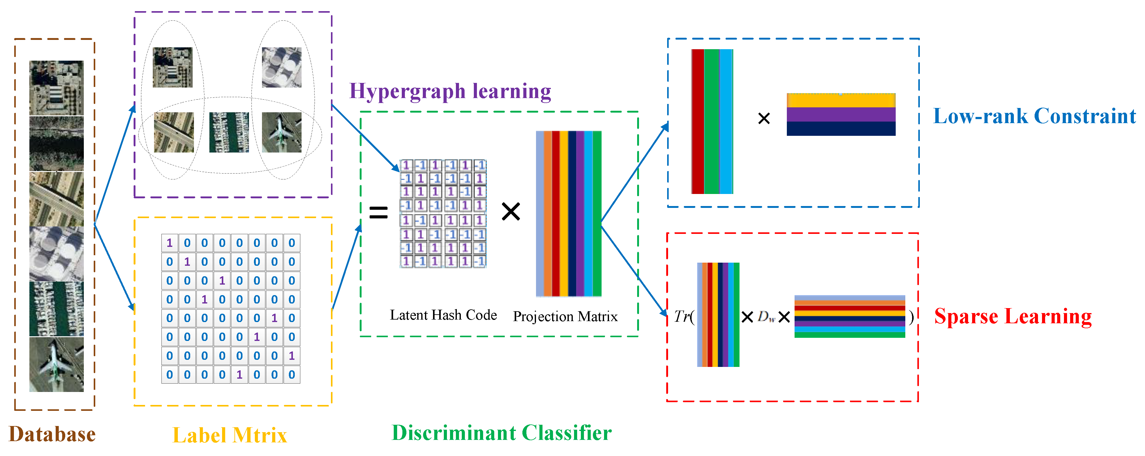
To address the aforementioned problems, new LHH is proposed to deal with large-scale RSIR tasks. The flowchart of the proposed LHH is shown in Figure 1, where we see that the proposed LHH is a shallow model, although its key components can also be easily considered in deep extensions of LHH. The main contributions of the proposed LHH are summarized as follows:

Figure 1. Illustration of the proposed low-rank hypergraph hashing (LHH).

(1)

The LHH employs a l_2-1 norm to constrain the projection matrix to reduce the noise and redundancy among features. In addition, low-rankness is also imposed on the projection matrix to exploit its global structure.

(2)

The LHH exploits the hypergraph to capture the high-order relationship among data, and is very suitable to explore the complex structure of RS images.

(3)

Finally, the proposed LHH is evaluated on three large-scale remote sensing datasets and one natural image dataset. The experimental results show that the proposed LHH outperforms some existing hashing methods in large-scale RSIR tasks.

The rest of the paper is organized as follows. The notation and related work are presented in Section 2. The proposed method is discussed in Section 3. The extensive experimental evaluations are presented in Section 4. Finally, a conclusion is given in Section 5.

2. Notation and Related Work

The notation of the paper and the recent advances of hashing techniques, low-rank analysis and hypergraph learning are reviewed in this section.

2.1. Notation

In this paper, we represent matrix and vector as a boldface italic letter, and scalar as a normal italic letter. For a matrix X = [x_ij], its i-th row and j-th column are denoted as xⁱ and x_j, respectively. We represent the transpose operator, the inverse and the trace operator of X as X^T, X^-1 and tr(X), respectively. We represent the Frobenius norm and l_2,1-norm of X, respectively. The important notations in the paper are summarized in Table 1.

Table 1. Important notation used in this paper.

Notation	Description
X	Data matrix
Y	Label matrix
W	Projection matrix
A	Hash code basis matrix
B	Hash code matrix
C	Hash code coefficient matrix
H	Hypergraph similarity matrix
L	Hypergraph Laplace matrix
M	Data basis matrix
N	Data coefficient matrix
n	Sample number
m	Sample dimensionality
n	Class number
l	Hash code length
r	Rank of projection matrix
k	Hyperedge number
t	Iteration number
λ1	Sparse regularization parameter
λ2	Hypergraph regularization parameter

2.2. Hashing Learning

Hashing has been a key step to facilitate large-scale image retrieval [24]. Essentially, hashing maps the high-dimensional data into a low-dimensional Hamming space while preserving similarity structure among data. The representative hashing methods include local sensitive hashing (LSH) [25], spectral hashing (SH) [26], partial randomness hashing (PRH) [14], supervised hashing with kernels (KSH) [27] and supervised discrete hashing (SDH) [12]. LSH [25] obtains hash functions via random projections. Original metrics are theoretically guaranteed to be preserved in the Hamming space, and LSH often requires long code length to get high precision. The SH [26] preserves the similarity distribution among data and the binary codes are imposed to be balanced and uncorrelated. PRH [14] establishes a partial stochastic strategy to enable good approximation and fast learning to construct hashing functions. KSH [27] maps the data into binary codes whose Hamming distance are minimized on similar pairs and maximized on dissimilar pairs. Based on the equivalence between optimizing the code inner product and Hamming distance, KSH can train the hash function efficiently. SDH [12] aims to learn the hash codes that are good for classification. To deal with the non-deterministic polynomial hard (NP-hard) binary constraint, the SDH develops a cyclic coordinate descent to generate good hash codes, which admits an analytical solution.

2.3. Low-Rankness Analysis

The low-rankness property is attracting more and more attention, since it enables the finding of low-rank structures from high-dimensional data that is corrupted with noise and outliers [28,29]. With low-rank constraints, the computational complexity can be greatly reduced. [30] has proved that low-rank regression equals regression in the subspace generated by linear discriminant analysis (LDA). Low-rank representation (LRR) [31] seeks to find the lowest rank representation where data can be represented by linear combinations of the basis in a given dictionary. To further enhance LRR, latent low-rank representation (LatLRR) [32,33] is proposed to recover the unobserved data in LRR.

Since low-rank optimization problem is a NP-hard problem, we instead solve the nuclear norm minimization problem via alternating direction method of multipliers (ADMM) [34]. Low-rank can be used in matrix decomposition due to its advantage in "de-correlation". Specifically, given a matrix X with the rank r, low-rank decomposition solves the following optimization problems:

$$\begin{array}{c}\underset{M,N}{\mathrm{argmin}}\mathit{X}\approx \mathit{M}\mathit{N}\\ \mathrm{s}.\mathrm{t}. r<\min \left\{m,n\right\},\mathit{X}\in {ℝ}_{m\times n},\mathit{M}\in {ℝ}_{m\times r}, \mathit{N}\in {ℝ}_{r\times n} \end{array}$$

(1)

It is evident that the size of X is larger than the sum of those of M and N. Therefore, the low rank matrix decomposition can remove the correlation among data, thereafter reducing the storage.

2.4. Hypergraph Learning

Since conventional graphs fail to exploit the relationships among data, the hypergraph has been widely used to characterize the complex relationships among complex data [22,23]. Specifically, a hypergraph generalizes the conventional graph where one edge can connect more than two vertices and capture high-order information. Different from simple graphs, hypergraphs contain local grouping information that is beneficial to clustering. In [35], Huang et al. construct hyperedges among images based on shape and appearance features in their region of interests (ROI), and perform spectral clustering for unsupervised image categorization. In [14], a transductive learning framework is introduced to further explore the correlations. This approach constructs a probabilistic hypergraph, and hypergraph ranking is further employed. To accelerate similarity search, the authors in [23] extend the traditional unsupervised hashing method to a hypergraph to capture the high-order information for social images. Besides, Bu et al. have modeled the relationship of different entities using the hypergraph for recommendation in the social-media community [36].

3. Proposed Low-Rank Hypergraph Hashing (LHH) Method

This section first introduces the proposed LHH. Then, Section 3.1 gives the notation and problem statement. The details of the proposed LHH are presented in Section 3.2. After this, Section 3.3 presents the optimization of the proposed LHH. Moreover, Section 3.4 introduces learning the hashing function. Finally, Section 3.5 presents the convergence analysis.

3.1. Problem Statement

Suppose that $\mathit{O}={\left\{{\mathit{o}}_i\right\}}_{i=1}^n$ is a set of images, and we are given its feature $\mathit{X}=\left[{\mathit{x}}^1;\dots ;{\mathit{x}}^n\right]\in {ℝ}_{n\times m}$, where m is the dimensionality and n is the number of the images. We represent the hash code matrix $\mathit{B}=\left[{\mathit{b}}^1;\dots ;{\mathit{b}}^n\right]\in {\left\{-1,1\right\}}^{n\times l}$, where ${\mathit{b}}^i\in {\left\{-1,1\right\}}^{1\times l}$ is the hash code of ${\mathit{o}}_i$ and l is the code length. The hash function HF(x) =sgn(F(x)) encodes x by l-bit hash code, where sgn (·) is the sign function, which outputs +1 for positive numbers and −1 otherwise. The LHH aims to learn B and the hash function HF to preserve the similarity structure of the images.

3.2. Low-Rank Hypergraph Hashing

To consider the supervised information, we regard learning the binary codes in the context of classification. We enable the binary codes to be optimal for the jointly learned classifier. Thus, the good binary codes are ideal for the classification.

Given binary code b, we adopt the following multi-class classification formulation

$$\mathit{y}=\mathit{G}\left(\mathit{b}\right)=\mathit{b}\mathit{W}=\left[\mathit{b}{\mathit{w}}_1,\dots , \mathit{b}{\mathit{w}}_c\right]$$

(2)

where $\mathit{W}=\left[{\mathit{w}}_1,\dots , {\mathit{w}}_c\right]\in {ℝ}^{l\times c}$, ${\mathit{w}}_k\in {ℝ}^{l\times 1}, k=1,\dots , c$ is the projection for class k and $\mathit{y}\in {ℝ}^{1\times c}$ is the label vector, and the maximum value indicates the assigned class of x.

We choose to optimize the following problem

$$\begin{array}{l}\underset{\mathit{B},\mathit{W}}{\min }{\displaystyle \sum }_{i=1}^n\mathit{L}\left({\mathit{y}}_{\mathit{i}}-{\mathit{b}}_{\mathit{i}}\mathit{W}\right)+{\lambda }_1\mathit{R}\left(\mathit{W}\right)\hfill \\ s.t. {\mathit{b}}_i\in {\left\{-1,1\right\}}^{1\times l},i=1,\dots ,n\hfill \end{array}$$

(3)

where L(·) is the loss function, R(W) is a regularizer and ${\lambda }_1$ is a regularization parameter. $\mathit{Y}={\left\{{\mathit{y}}_i\right\}}_{i=1}^n\in {ℝ}^{n\times c}$ is the ground truth label matrix, where $y_{ik}$=1 if x_i belongs to class k and 0 otherwise.

Equation (3) is flexible, and we can define any loss function for L(·). For simplicity, we can choose the simple l₂ loss, which minimizes the difference between the label Y and prediction G(b). The problem in Equation (3) can be transformed into the following problem:

$$\begin{array}{l}\underset{\mathit{B},\mathit{W}}{min}{\left|\right|\mathit{Y}-\mathit{B}\mathit{W}\left|\right|}_F^2+{\lambda }_1{\left|\right|\mathit{W}\left|\right|}_F^2\hfill \\ s.t. \mathit{B}\in {\left\{-1,1\right\}}^{n\times l}\hfill \end{array}$$

(4)

To enable the coefficients of data in the same space to be highly correlated, we apply the low rank constraint to capture the global structure of the whole data. In addition, the low-rank structure can relieve the impact from noises, and makes regression more accurate [37,38]. In order to consider the low-rank structure of W, we need to make:

$$rank\left(\mathit{W}\right)=r\le min\left(l,c\right)$$

(5)

We decompose W into two low-rank matrices, i.e., $\mathit{W}=\mathit{A}\mathit{C}$, where $\mathit{A}\in {ℝ}^{l\times r}, \mathit{C}\in {ℝ}^{r\times c}$, and r is the rank of W. Then, Equation (4) can be further transformed into

$$\begin{array}{l}\underset{\mathit{A},\mathit{B},\mathit{C}}{min}{\left|\right|\mathit{Y}-\mathit{B}\mathit{A}\mathit{C}\left|\right|}_F^2+{\lambda }_1{\left|\right|\mathit{A}\mathit{C}\left|\right|}_F^2\hfill \\ s.t.\mathit{B}\in {\left\{-1,1\right\}}^{n\times l}, \mathit{A}{\mathit{A}}^{\mathit{T}}=\mathit{I}\hfill \end{array}$$

(6)

where $\mathit{A}{\mathit{A}}^{\mathit{T}}=\mathit{I}$($\mathit{I}={ℝ}^{r\times r}$), which is introduced for identifiability. Besides, we additionally enforce the sparsity, i.e., l₂₁–norm for feature selection by [39]. Thus, the above problem is rewritten as:

$$\begin{array}{l}\underset{\mathit{A},\mathit{B},\mathit{C}}{min}{\left|\right|\mathit{Y}-\mathit{B}\mathit{A}\mathit{C}\left|\right|}_F^2+{\lambda }_1{\left|\right|\mathit{A}\mathit{C}\left|\right|}_{2,1}^2\hfill \\ s.t.\mathit{B}\in {\left\{-1,1\right\}}^{n\times l}, \mathit{A}{\mathit{A}}^{\mathit{T}}=\mathit{I}\hfill \end{array}$$

(7)

In Equation (7), we consider both low-rankness and sparsity to learn the regression coefficient matrix. Low-rankness deals with the noises, and the l_2,1-norm selects features by setting some rows of W to be zero.

Until now, we do not consider the similarity structure among data. If two samples are similar, we need to ensure that two corresponding binary codes are close. To preserve the original local similarity structure, we aim to minimize

$$minRf\left(\mathit{W}\right)=\frac{1}{2}{\displaystyle \sum }_{i,j}^n{\mathit{s}}_{i,j}||{\widehat{\mathit{y}}}^i-{\widehat{\mathit{y}}}^j||{}_2^2$$

(8)

where S (${\mathit{s}}_{i,j}\in \mathit{S}$) is the similarity matrix that records similarities among data, in which ${\mathit{s}}_{i,j}$ represents the relationship between the i-th and the j-th sample. Normally, we use the following formulation to construct graphs

$$f\left(\mathit{a},\mathit{b}\right)=exp\left(-\frac{\left|\right|\mathit{a}-\mathit{b}\left|\right|{}_2^2}{2{\sigma }^2}\right)$$

(9)

where $\sigma$ is the kernel width and the term $\left|\right|\mathit{a}-\mathit{b}\left|\right|{}_2^2$ denotes the distance between two samples.

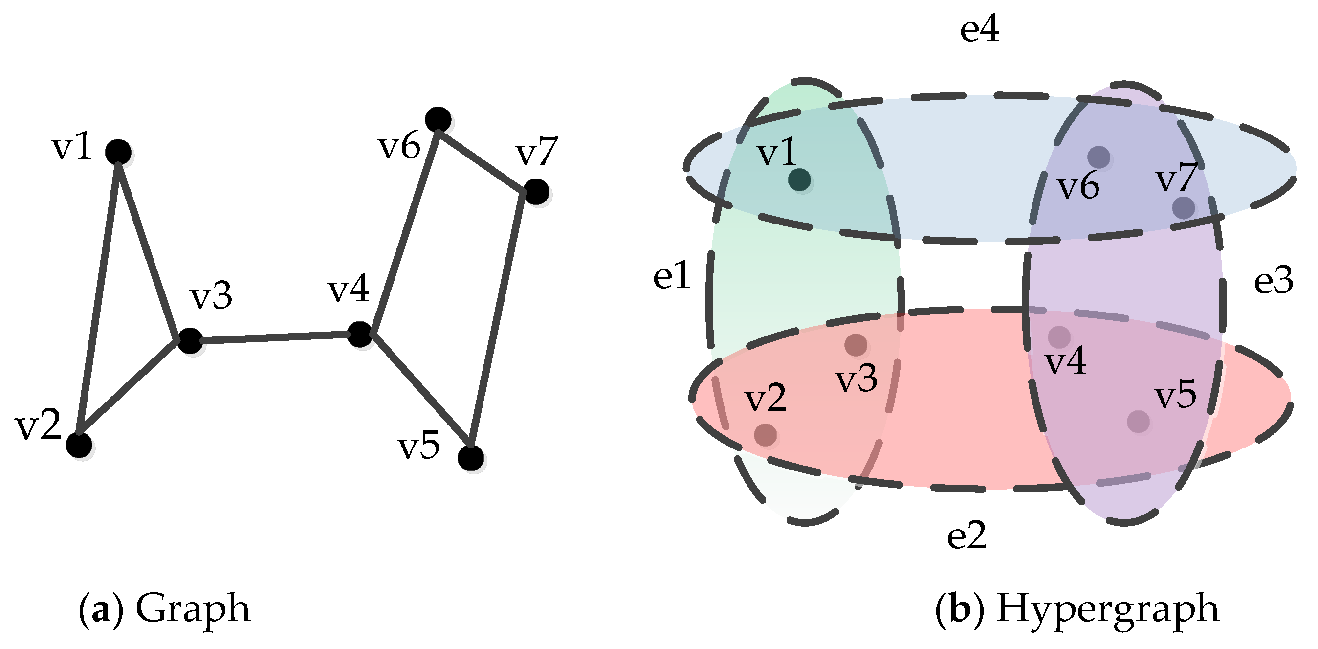
Here we instead use the hypergraph to measure the similarity among data. Figure 2 shows the distinction between a normal graph and hypergraph. As can be seen, the normal graph only connects two samples, while a hypergraph can connect more than two samples. Therefore, a hypergraph can reveal more complex relationships among data [23]. We formulate the incidence matrix H between the vertices and the hyperedges of the hypergraph as:

$$\mathit{H}\left(v,e\right)=\{\begin{array}{l}\begin{array}{cc}1,& \mathrm{if} v\in e\end{array}\hfill \\ \begin{array}{cc}0,& \mathrm{otherwise}\end{array}\hfill \end{array}$$

(10)

Figure 2. Illustration of a graph and hypergraph.

The degree $d\left(v\right)$ of vertex v and the degree $\delta \left(e\right)$ of hyperedge are defined as follows:

$$\begin{array}{l}d\left(v\right)={\displaystyle \sum }_e\mathit{S}\left(e\right)\mathit{H}\left(v,e\right)\hfill \\ \delta \left(e\right)={\displaystyle \sum }_v\mathit{H}\left(v,e\right)\hfill \end{array}$$

(11)

With the above definition, the normalized distance between $v_i$ and $v_j$ on $e_k$ is $\frac{w\left(e_k\right)}{\delta \left(e_k\right)}{\left(\frac{y_i}{\sqrt{d\left(v_i\right)}}-\frac{y_j}{\sqrt{d\left(v_j\right)}}\right)}^2$. To preserve the similarity of hash codes, we aim to map data on the same hyperedge into more similar hash codes. Thus, we seek the hash codes by minimizing the average Hamming distance between hash codes of data on the same hyperedge:

$$\begin{array}{l}\underset{B}{\min }\frac{1}{2}{\displaystyle \sum }_{e_k\in E}{\displaystyle \sum }_{v_i,v_j\in e_k}\frac{S\left(e_k\right)}{\delta \left(e_k\right)}{\left(\frac{{\mathit{b}}_i}{\sqrt{d\left(v_i\right)}}-\frac{{\mathit{b}}_j}{\sqrt{d\left(v_j\right)}}\right)}^2\hfill \\ \mathrm{s}.\mathrm{t}. {\mathit{b}}_i\in {\left\{-1,1\right\}}^{1\times l},i=1,\dots ,n\hfill \end{array}$$

(12)

By introducing the hypergraph Laplacian, we further rewrite Equation (12) as

$$\begin{array}{l}\underset{B}{\min }\mathrm{tr}\left({\mathit{B}}^T\mathit{L}\mathit{B}\right)\hfill \\ \mathrm{s}.\mathrm{t}. \mathit{B}\in {\left\{-1,1\right\}}^{n\times l}\hfill \end{array}$$

(13)

where the hypergraph Laplacian matrix $\mathit{L}=\mathit{I}-{\mathit{D}}_v^{-\frac{1}{2}}\mathit{H}{\mathit{D}}_e^{-1}{\mathit{H}}^T{\mathit{D}}_v^{-\frac{1}{2}}$, I is the identity matrix, H is the incidence matrix and ${\mathit{D}}_{\mathit{v}}$ and ${\mathit{D}}_{\mathit{e}}$ are diagonal matrices, where the diagonal element of ${\mathit{D}}_{\mathit{v}}$ and ${\mathit{D}}_{\mathit{e}}$are degrees of the hypergraph vertex $d\left(v_i\right)$ and hyperedge $\delta \left(e_i\right)$, respectively.

Combining Equations (7) and (13), the final objective function of LHH is defined as:

$$\begin{array}{l}\underset{A,B,C}{\min }\Vert \mathit{Y}-\mathit{B}\mathit{A}\mathit{C}{\Vert }_F^2+{\lambda }_1\Vert \mathit{A}\mathit{C}{\Vert }_{2,1}+{\lambda }_2\mathrm{tr}\left({\mathit{B}}^T\mathit{L}\mathit{B}\right)\hfill \\ \mathrm{s}.\mathrm{t}.\mathit{B}\in {\left\{-1,1\right\}}^{n\times l}, \mathit{A}{\mathit{A}}^{\mathit{T}}=\mathit{I}\hfill \end{array}$$

(14)

where ${\lambda }_2$ is a regularization parameter. In Equation (14), to learn high-quality binary codes, the first term learns the classifier with a binary code, the second term minimizes the l_2,1-norm of the projection matrix to explore its low-rankness and sparsity, and the third term preserves the intrinsic complex structure of data via a hypergraph.

3.3. Optimization Algorithm

It is clear that Equation (14) is difficult to find a global solution for, as it is nonconvex. We alternatively solve the sub-problems for the following variables.

(1) C-step: Update C by fixing A and B.

Algorithm 1 Curvilinear Search Algorithm Based on Cayley Transformation

Input: initial point ${\mathit{A}}^{\left(0\right)}\in {ℝ}^{l\times r}$, matrix B, C, hash code length l

Output: A(t).

1: Initialize t = 0, $\mathsf{\epsilon }>0$ and ${\lambda }_1=1,{\lambda }_2=1\mathrm{e}-2$.

2: Repeat

3:  Compute the gradient according to (18);

4:  Generate the skew-symmetric matrix $\mathit{F}={\mathit{G}}^T\mathit{A}-{\mathit{A}}^T\mathit{G}$;

5:  Compute the step size ${\tau }_t$, that satisfies the Armijo-Wolfe conditions [33] via the line search along the path ${\mathit{J}}_t\left(\tau \right)$ defined by (19);

6:  Set ${\mathit{A}}^{\left(t+1\right)}=\mathit{J}\left({\tau }_t\right)$;

7:  Update t = t + 1;

8: Until convergence

In this case, the objective function is simplified as:

$$\underset{\mathit{C}}{\min }\mathrm{Loss}\left(\mathit{C}\right)=\left|\right|\mathit{Y}-\mathit{B}\mathit{A}\mathit{C}\left|\right|{}_F^2+{\lambda }_1\left|\right|\mathit{A}\mathit{C}\left|\right|{}_{2,1}$$

(15)

Equation (15) can be rewritten as:

$$\underset{\mathit{C}}{\min }\mathrm{Loss}\left(\mathit{C}\right)=-2\mathrm{tr}\left({\mathit{C}}^T{\mathit{A}}^T{\mathit{B}}^T\mathit{Y}\right)+2\mathrm{tr}\left({\mathit{C}}^T{\mathit{A}}^T{\mathit{B}}^T\mathit{B}\mathit{A}\mathit{C}\right)+{\lambda }_1\Vert AC{\Vert }_{2,1}$$

(16)

We have the derivative of Equation (16) with respect to C equal to 0, and receive

$$\mathit{C}={\left({\mathit{A}}^T{\mathit{B}}^T\mathit{B}\mathit{A}+{\lambda }_1{\mathit{A}}^T{\mathit{D}}_w\mathit{A}\right)}^{-1}{\mathit{A}}^T{\mathit{B}}^T\mathit{Y}$$

(17)

where ${\mathit{D}}_{\mathit{W}}=\frac{1}{2\Vert w^i{\Vert }_2}=\frac{1}{2\Vert {\left(AC\right)}^i{\Vert }_2}$ is a diagonal matrix.

(2) A-step: Update A by fixing B and C.

It is hard to obtain an optimal solution in Equation (14) with respect to A, due to the orthogonal constraint. Here we apply a gradient descent with a curvilinear search to seek a locally optimal solution.

First, we denote G as the gradient of Equation (16) with respect to A, and it is defined as:

$$\mathit{G}=-2{\mathit{B}}^T\mathit{Y}{\mathit{C}}^T+2{\mathit{B}}^T\mathit{B}\mathit{A}\mathit{C}{\mathit{C}}^T+2{\lambda }_1{\mathit{D}}_{\mathit{W}}\mathit{A}\mathit{C}{\mathit{C}}^T$$

(18)

A skew-symmetric matrix is defined as $\mathit{F}={\mathit{G}}^T\mathit{A}-{\mathit{A}}^T\mathit{G}$. The next point is decided by a Crank-Nicolson scheme

$$\mathit{J}\left(\tau \right)=\mathit{A}-\frac{\tau }{2}{\mathit{F}}^T\left(\mathit{A}+\mathit{J}\left(\tau \right)\right)$$

(19)

where $\tau$ is the step size. We can get a closed-form solution of $J\left(\tau \right)$:

$$\begin{array}{c}\mathit{J}\left(\tau \right)=\mathit{A}\mathit{M},\\ \mathit{M}=\left(\mathit{I}-\frac{\tau }{2}{\mathit{F}}^{\mathrm{T}}\right){\left(\mathit{I}+\frac{\tau }{2}{\mathit{F}}^{\mathrm{T}}\right)}^{-1}\end{array}$$

(20)

Here, Equation (20) is called the Cayley transformation [33,40,41]. The iteration terminates when τ_t satisfies the Armijo-Wolfe condition. The algorithm solving the sub-problem is illustrated in Algorithm 1.

(3) B-step: Update B by fixing A and C.

The objective function is simplified as follows:

$$\begin{array}{l}\underset{\mathit{B}}{\min }\mathrm{Loss}\left(\mathit{B}\right)=\mathrm{tr}\left[{\left(\mathit{Y}-\mathit{B}\mathit{A}\mathit{C}\right)}^T\left(\mathit{Y}-\mathit{B}\mathit{A}\mathit{C}\right)\right]+{\lambda }_2\mathrm{tr}\left({\mathit{B}}^T\mathit{L}\mathit{B}\right)\hfill \\ \mathrm{s}.\mathrm{t}.\mathit{B}\in {\left\{-1,1\right\}}^{n\times l} \hfill \end{array}$$

(21)

The above problem is challenging due to the discrete constraint, and it has no closed-form solution. Inspired by the recent study in nonconvex optimization, we optimize Equation (21) with the proximal gradient method, which iteratively optimizes a surrogate function. In the j-th iteration, we define a surrogate function $\stackrel{\wedge }{{\mathrm{Loss}}_j}\left(\mathit{B}\right)$ that is a discrete approximation of $\mathrm{Loss}\left(\mathit{B}\right)$ at the point ${\mathit{B}}^{\left(\mathrm{j}\right)}$. Given ${\mathit{B}}^{\left(\mathrm{j}\right)}$, the next discrete point is obtained by optimizing:

$${\mathit{B}}^{\left(j+1\right)}\in {\mathrm{argmax}}_{\mathit{B}\in {\left\{-1,1\right\}}^{n\times l}}\stackrel{\wedge }{{\mathrm{Loss}}_j}\left(\mathit{B}\right):=\mathrm{Loss}\left({\mathit{B}}^{\left(j\right)}+⟨\nabla \mathrm{Loss}\left({\mathit{B}}^{\left(j\right)}\right),\mathit{B}-{\mathit{B}}^{\left(j\right)}⟩\right)$$

(22)

Note that $\nabla \mathrm{Loss}\left({\mathit{B}}^{\left(j\right)}\right)$ may include zero entries and that multiple solutions for ${\mathit{B}}^{\left(j+1\right)}$ may exist, thus we introduce function$\mathrm{Cf}\left(\mathrm{x}, \mathrm{y}\right)=\{\begin{array}{c}x,x\ne 0\\ y,y=0\end{array}$ to eliminate the zero entries. The updated rule for ${\mathit{B}}^{\left(j+1\right)}$ is defined as [42,43]:

Algorithm 2 Low-Rank Hypergraph Hashing

Input: label matrix $\mathit{Y}\in {ℝ}^{\mathrm{n}\ast c}$, hash code length l, hyperedge number k;

Output: A(t), B(t), C(t);

1: Initialize ${\mathit{A}}^{\left(0\right)}\in {ℝ}^{l\times r}$, ${\mathit{B}}^{\left(0\right)}\in {\left\{-1, 1\right\}}^{n\times l}$, ${\mathit{C}}^{\left(0\right)}\in {ℝ}^{r\times c}$, $\mathit{H}\in {ℝ}^{n*k}$;

2: Initialize t=0, $\mathsf{\epsilon }>0$, and ${\lambda }_1=1$, ${\lambda }_2=1\mathrm{e}-2$;

3: Repeat

4:  C-step: Update C(t) using (17);

5:  A-step: Update A(t) by Algorithm 1;

6:  B-step: Update B(t) using (23);

7:  Update t=t+1;

8: Until convergence

$${\mathit{B}}^{\left(j+1\right)}≔\mathrm{sgn}\left(C\left(\nabla \mathrm{Loss}\left({\mathit{B}}^{\left(j\right)}\right),{\mathit{B}}^{\left(j\right)}\right)\right)=\mathrm{sgn}\left(\mathrm{Cf}\left(-2\mathit{Y}{\left(\mathit{A}\mathit{C}\right)}^T+2\mathit{B}\left(\mathit{A}\mathit{C}\right){\left(\mathit{A}\mathit{C}\right)}^T+2{\lambda }_2\mathit{L}\mathit{B},{\mathit{B}}^{\left(j\right)}\right)\right)$$

(23)

The learning algorithm of LHH is shown in Algorithm 2.

3.4. Hash Function Learning

The optimal hash code has been learned, and we need to further learn a mapping from the original space to Hamming space. Here we assume that there is a linear mapping between the two spaces, and the transformation matrix is learned by optimizing the following problem [12]:

$$\underset{\mathit{P}}{min}\left|\right|\mathit{B}-\mathit{X}\mathit{P}\left|\right|{}_F^2$$

(24)

In Equation (24), it measures the fitting error between data and hash codes. The solution of the problem admits the following form:

$$\mathit{P}={\left({\mathit{X}}^T\mathit{X}\right)}^{-1}{\mathit{X}}^T\mathit{B}$$

(25)

Finally, the hash function is defined as

$$\mathit{H}\mathit{F}=sgn\left(x\mathit{P}\right),$$

(26)

where x is an arbitrary sample.

3.5. Convergence Analysis and Computational Complexity Analysis

Firstly, we discuss the convergence of LHH, which is presented in the following theorem.

Theorem 1: The alternating iteration scheme of Algorithm 2 monotonically reduces the objective function value of Equation (14), and Algorithm 2 converges to a local minimum of Equation (14).

Proof: LHH includes three sub-problems. The sub-problem C is convex, thus it clearly has the optimal solution. The sub-problems with respect to A and B are non-convex, but A and B steps decrease the objective function value. Thus, Algorithm 2 decreases the objective function value in each step. In addition, the objective function value is non-negative. Thus, Algorithm 2 can converge to a local optimal solution of LHH.

Then, we present the computational complexity of the proposed LHH method. The computational complexity of LHH mainly consists of the following several parts. In the step of updating $\mathit{A}$, its complexity is $\mathcal{O}\left(nlr\right)$. In the step of updating $\mathit{A}$, due to the orthogonal constraint, we use the Cayley transformation for solving this problem. Computing the gradient of $\mathit{A}$ requires $\left(n{l}^2+nlc\right)$ and updating $\mathit{A}$ for each iteration is $\mathcal{O}\left(4n{l}^2+l^3\right)$ [40]. Thus, the complexity of optimizing $\mathit{A}$ is $\mathcal{O}\left(t1\left(n{l}^2+nlc+4n{l}^2+l^3\right)\right)$, where $t1$ is the number of iterations for updating $\mathit{A}$. In the step of updating $\mathit{B}$, its complexity is $\mathcal{O}\left(n^{2}l\right)$, and it is time-consuming, as it contains hypergraph Laplacian matrix computing. In summary, the total computational complexity of LHH is $\mathcal{O}\left(t\left(nlr+n^{2}l+t1\left(n{l}^2+nlc+4n{l}^2+l^3\right)\right)\right)$, where $t$ is the number of total iterations in Algorithm 2. Finally, the computational complexity of hashing mapping matrix $\mathit{P}$ requires the time complexity of $\mathcal{O}\left(n{d}^2+ndl\right)$. For the query part, the computational cost for encoding any query $x$ is $\mathcal{O}\left(cd\right)$.

4. Experiments

We compare the proposed method with some state-of-the-art methods on four benchmark datasets, and their performance is evaluted in large-scale remote-sensing retrieval tasks.

4.1. Datasets

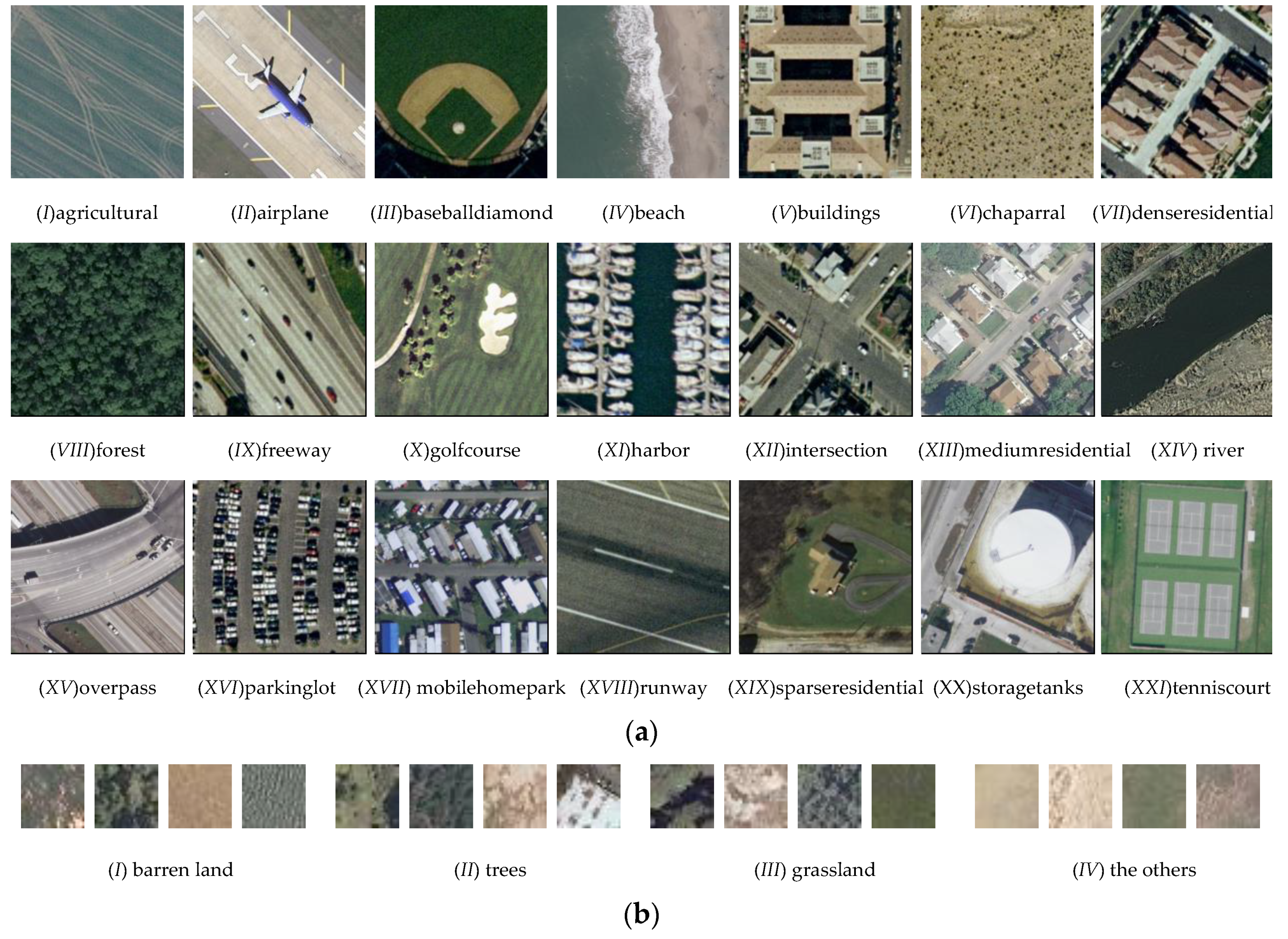
We adopt four benchmark datasets: UC Merced Land Use Dataset (UCMD) [44]; SAT4 [45]; SAT6 [45]; and CIFAR10 [46]. Their descriptions are as follows:

• UCMD is generated by manually labeling aerial image scenes, and it covers 21 land cover categories. More specifically, each land cover category includes 100 images of 256 × 256 pixels. The spatial resolution of this public domain imagery is 0.3 meters. Here we randomly sample 420 samples as the query set, and use the remaining 1680 samples for training.
• SAT4 consists of a total of 500,000 image patches covering four broad land cover classes. These include barren land, grassland, trees and a class that consists of all land cover classes other than the above three. Each image patch is size normalized to 28 × 28 pixels, and the spatial resolution of each pixel is 1 m. we randomly select 100,000 samples as the query set, and the other 400,000 samples as a training set.
• SAT6 consists of a total of 405,000 image patches covering six broad land cover classes. These include barren land, buildings, grassland, roads, trees and water bodies. The image size and spatial resolution of SAT6 are similar with these of SAT4. We randomly select 81,000 samples as the query set, and the other 324,000 samples as a training set.
• CIFAR10 dataset consists of sixty thousand 32 × 32 color images of 10 classes and 6,000 images in each class. We randomly select 10,000 samples as the query set, and the remaining 50,000 samples as a training set.

The statistics of the four datasets are summarized in Table 2, and some sample images are presented in Figure 3.

Table 2. Statistics and several parameter settings of four datasets.

	UCMD	SAT4	SAT6	CIFAR10
Dataset Size (n)	2100	500,000	405,000	60,000
Training Set	1680	400,000	324,000	50,000
Query Set	420	100,000	81,000	10,000
Image Size	256 × 256	28 × 28	28 × 28	32 × 32
Class Number (c)	21	4	6	10
Rank of Projection Matrix (r)	10	2	3	5
Hyperedge Number (k)	21	4	6	10

Figure 3. Sample images of four datasets: (a) UCMD; (b) SAT4; (c) SAT6; and (d) CIFAR10.

4.2. Experimental Setting

To verify the effectiveness of the proposed low-rank hypergraph hashing (LHH), we select several hashing methods for the performance comparison, including local sensitive hashing (LSH) [25], spectral hashing (SH) [26], partial randomness hashing (PRH) [14], HSH [21], supervised hashing with kernels (KSH) [27] and supervised discrete hashing (SDH) [12].

In the experiment, the samples are represented as 512-dimensional gistification (GIST) vectors. The experiments are conducted on a standard PC with Intel Core i7-8550U, CPU 2.70 GHz and 8GB RAM. In the experiment, ${\lambda }_1$ and ${\lambda }_2$ are empirically set as 1 and 0.01 respectively. Other parameter setting of the used four datasets is summarized in Table 2.

The retrieval performance is measured with two widely used metrics: mean average precision (mAP) and Precision-Recall (P-R) curve [47]. The mAP score is calculated by

$$mAP=\frac{1}{\left|Q\right|}{{\displaystyle \sum }}_{q=1}^{\left|Q\right|}\frac{1}{L_q}{{\displaystyle \sum }}_{r=1}^R{P}_q\left(r\right){\delta }_q\left(r\right)$$

(27)

where $q\in Q$ is a query, and $\left|Q\right|$ is the volume of query set. $L_q$ is the number of the true neighbors in the retrieved list. $P_q\left(r\right)$ denotes the precision of the top r retrieved results, ${\delta }_q\left(r\right)=1$ if the r-th result is the true neighbor, and 0 otherwise [48].

4.3. Performance Evaluation

4.3.1. Qualitative Analysis

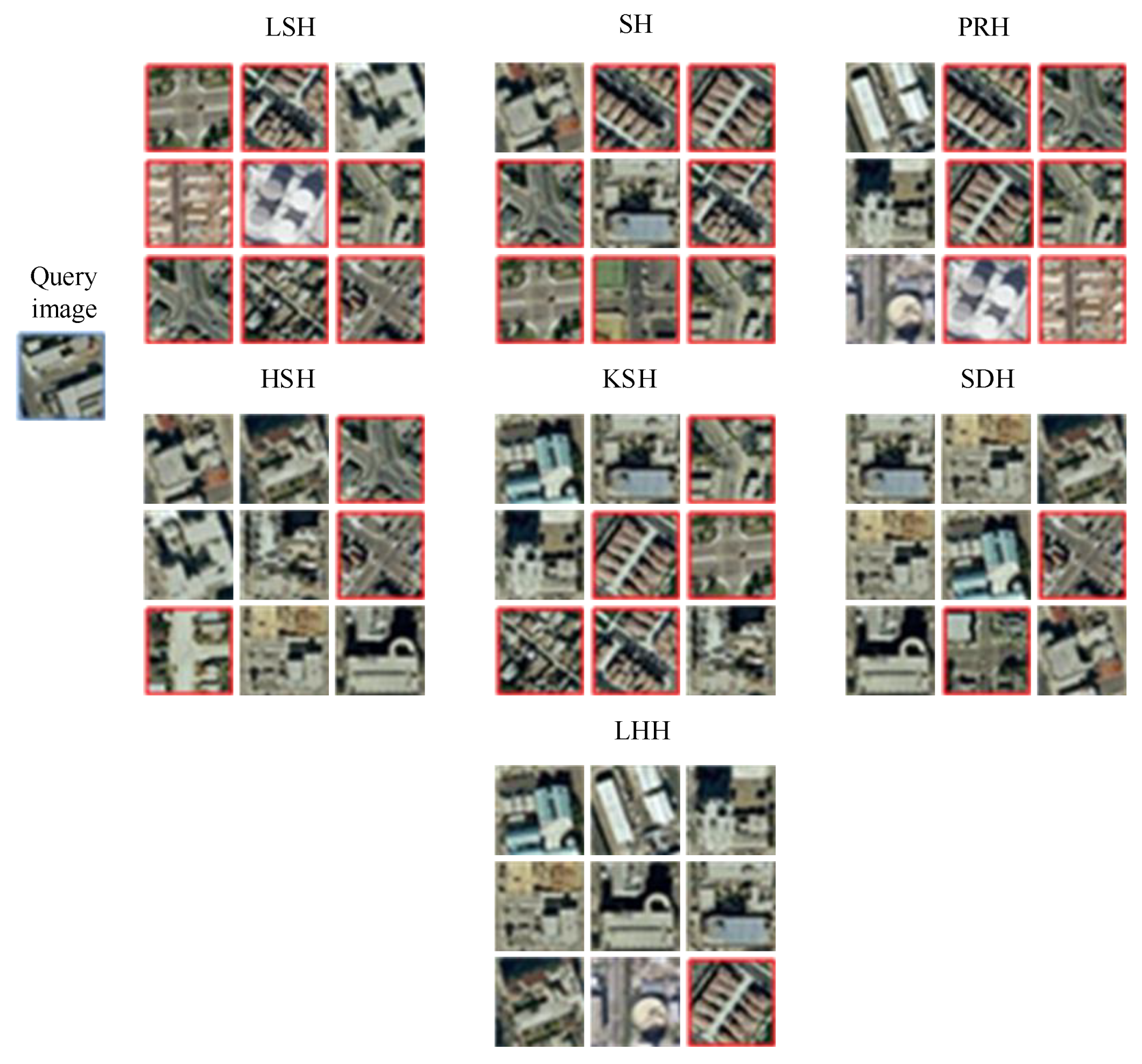
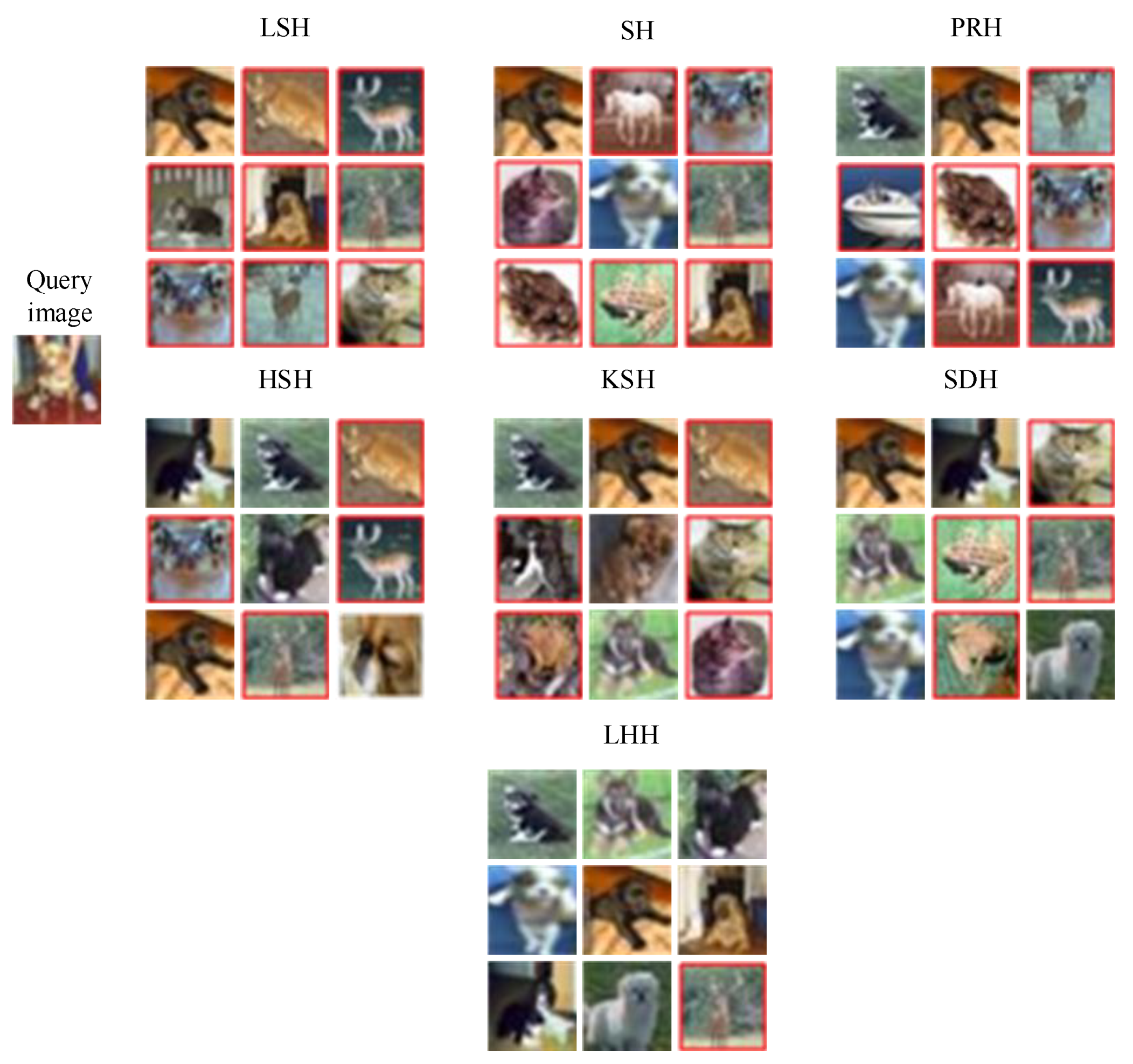
We illustrate the retrieval results of several hashing methods on UCMD and CIFAR10 in Figure 4 and Figure 5 respectively. Figure 4 illustrates the retrieved images of ‘building’ in UCMD, and Figure 5 illustrates the retrieved images of ‘dog’ in CIFAR10. The top nine images are returned, and the false images are with red rectangles.

Figure 4. Visualized retrieval results on the UCMD by six hashing methods with hash codes of 32 bits.

Figure 5. Visualized retrieval results on the CIFAR10 by six hashing methods with hash codes of 32 bits.

From Figure 4 and Figure 5, we can see that the proposed LHH can retrieve the most images among all the methods. LSH, SH and PRH retrieve 2–3 correct images, and HSH, KSH and SDH retrieve more than five similar images. The experiment validates the effectiveness of LHH.

4.3.2. Quantitative Analysis

(1) The comparison of mAP in several hashing methods under different datasets is shown in Table 3, Table 4, Table 5 and Table 6.

Table 3. Comparison of mAP with different hash code lengths on UCMD.

	Method	LSH	SH	PRH	HSH	KSH	SDH	LHH
Code Length
8-bits		0.1256	0.1394	0.1354	0.2395	0.2791	0.2684	0.3102
16-bits		0.1375	0.1479	0.1483	0.2468	0.2913	0.2897	0.3385
32-bits		0.1421	0.1534	0.1594	0.2587	0.3147	0.3214	0.3573
64-bits		0.1476	0.1589	0.1718	0.2671	0.3278	0.3348	0.3760

Table 4. Comparison of mAP with different hash code lengths on SAT4.

	Method	LSH	SH	PRH	HSH	KSH	SDH	LHH
Code Length
8-bits		0.3147	0.3086	0.3980	0.5551	0.5037	0.5467	0.6046
16-bits		0.3175	0.3149	0.4023	0.5632	0.5112	0.5589	0.6295
32-bits		0.3197	0.3218	0.4095	0.5729	0.5268	0.5727	0.6573
64-bits		0.3209	0.3256	0.4078	0.5756	0.5189	0.5671	0.6922

Table 5. Comparison of mAP with different hash code lengths on SAT6.

	Method	LSH	SH	PRH	HSH	KSH	SDH	LHH
Code Length
8-bits		0.3387	0.3242	0.5054	0.6237	0.5941	0.6189	0.6592
16-bits		0.3438	0.3317	0.5117	0.6319	0.6011	0.6348	0.6727
32-bits		0.3417	0.3478	0.5172	0.6402	0.6147	0.6514	0.7035
64-bits		0.3422	0.3449	0.5184	0.6446	0.6214	0.6621	0.7333

Table 6. Comparison of mAP with different hash code lengths on CIFAR10.

	Method	LSH	SH	PRH	HSH	KSH	SDH	LHH
Code Length
8-bits		0.1214	0.1648	0.2185	0.3919	0.3726	0.4367	0.4618
16-bits		0.1256	0.1687	0.2256	0.4031	0.4017	0.4613	0.4845
32-bits		0.1302	0.1724	0.2336	0.4163	0.4225	0.4967	0.5034
64-bits		0.1287	0.1693	0.2312	0.4203	0.4412	0.5111	0.5259

In Table 3, Table 4, Table 5 and Table 6, it is clearly observed that the LHH generally achieves the best performance. The SDH and KSH have similar results, where the KSH is better than the SDH on UCMD. Moreover, the SDH outperforms the KSH on the SAT4, SAT6 and CIFAR10 datasets. The HSH has a satisfactory performance on both the SAT4 and SAT6 datasets. For the other two methods, the PRH is generally superior to LSH and SH. Therefore, these results indicate that the LHH can have a promising retrieval performance on these four datasets.

(2) Figure 6 gives the comparison of P-R curves of six hashing methods under different datasets. In Figure 6, the P-R curve of LHH is mostly above than those of the other methods—thus LHH can obtain a larger area under curve (AUC), which is important for evaluating information retrieval. The performances of LSH, SH and PRH are worst, as their AUC areas are the smallest. The AUC areas of HSH are smaller than those of KSH and SDH, indicating that HSH underperforms KSH and SDH. The above results demonstrate the superiorities of the proposed LHH over the comparisons in large-scale retrieval tasks.

Figure 6. P-R curves of several hashing methods on (a) UCMD; (b) SAT4; (c) SAT6; and (d) CIFAR10.

4.4. Convergence Analysis

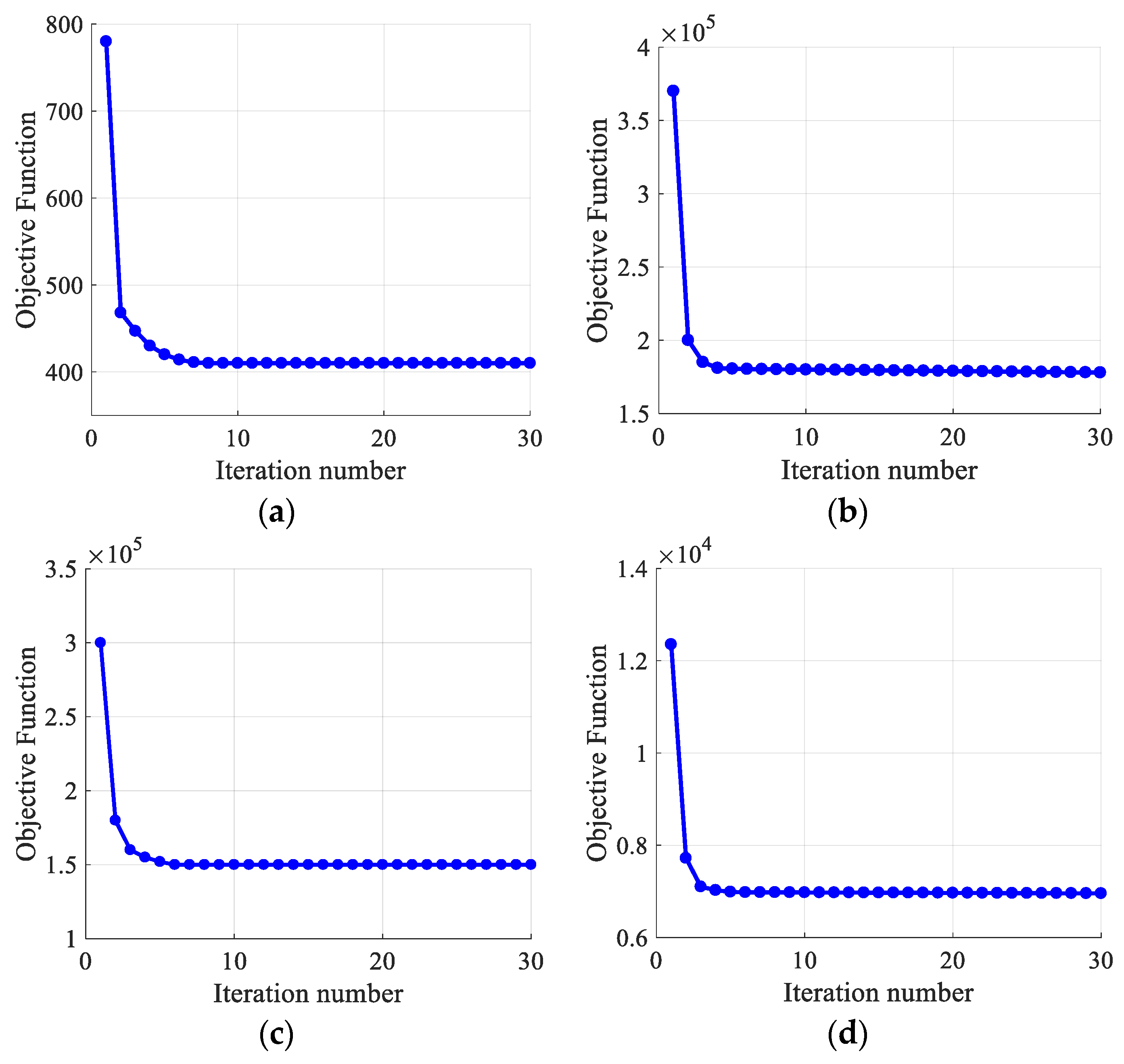
This section empirically studies the convergence of LHH. Figure 7 illustrates the convergence curves of LHH on these data sets. From Figure 7, we can clearly see that LHH quickly converges within around eight iterations. The empirical results corroborate Theorem 1.

Figure 7. The convergence analysis of LHH: (a) UC Merced Land Use Dataset (UCMD); (b) SAT4; (c) SAT6; and (d) CIFAR10.

4.5. Parameter Analysis

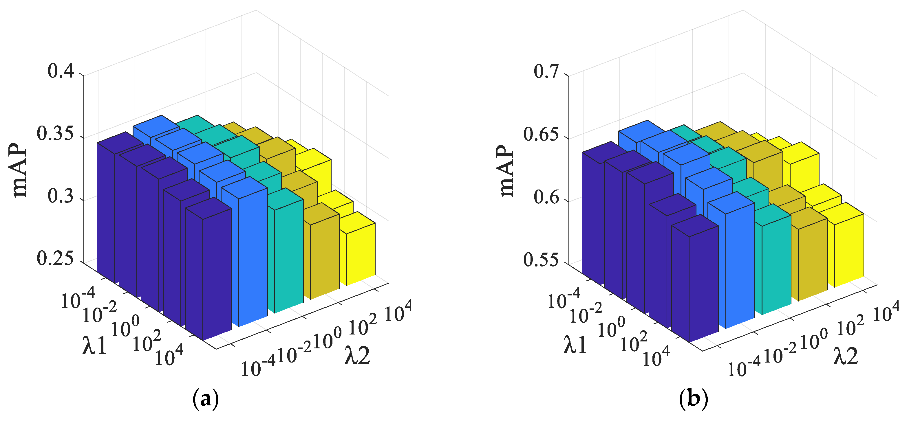
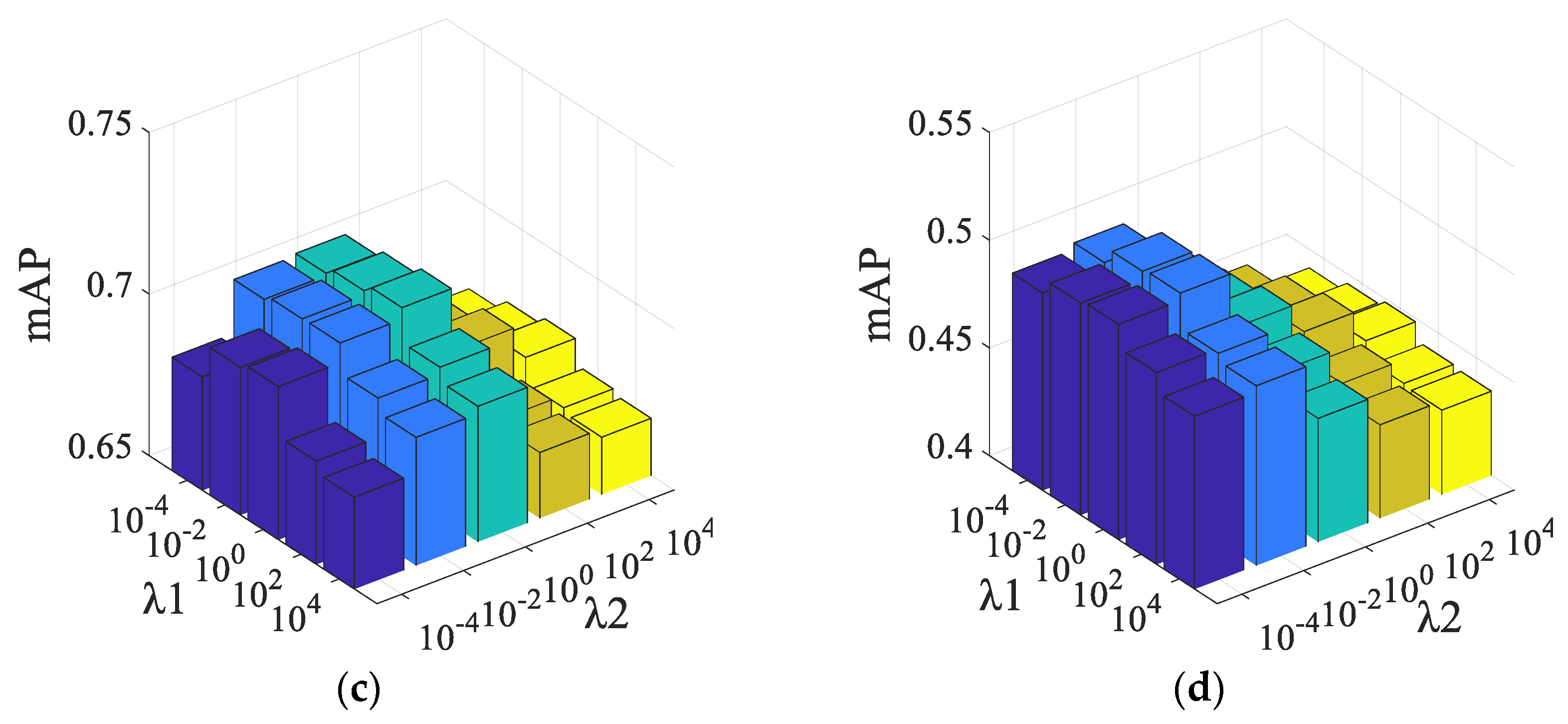
We discuss the sensitivity of the sparse regularization parameter ${\lambda }_1$ and hypergraph regularization parameter ${\lambda }_2$ in the proposed LHH. We show their influences on the mAP with a 32-bit code. In the experiment, ${\lambda }_1$ and ${\lambda }_2$ are varied from the range of [10⁻⁴, 10⁻², 10⁰, 10², 10⁴]. From Figure 8, we see that the mAP slightly changes with the two parameters. As ${\lambda }_1$and ${\lambda }_2$ increase, mAP slowly rises and then drops on four datasets. The mAP change with ${\lambda }_2$ is larger than that of ${\lambda }_1$. In general, the LHH can achieve acceptable results on the four datasets when ${\lambda }_1$, ${\lambda }_2$ ∈ [0.01,1]. These results demonstrate that sparse and hypergraph terms can help improve the retrieval.

Figure 8. Parameter analysis of ${\lambda }_1$ and ${\lambda }_2$ in LHH on: (a) UCMD; (b) SAT4; (c) SAT6; and (d) CIFAR10.

5. Discussion

The experimental results on four datasets reveal the following interesting points:

• Section 4.3.1 qualitatively shows that the proposed low-rank hypergraph hashing (LHH) has better retrieval performance on large-scale remote sensing (RS) image datasets. Specifically, LHH can retrieval more correct images than the comparison methods, as shown in Figure 4 and Figure 5.
• Section 4.3.2 quantitatively reveals that the proposed LHH is obviously superior than the existing methods on four large-scale datasets, including three remote sensing and one natural image dataset. Specifically, Table 3, Table 4, Table 5 and Table 6 illustrates that LHH has a higher mean average precision (mAP) than comparison methods, and Figure 6 illustrates that LHH also has better Precision-Recall (P-R) curves.
• Section 4.4 shows that LHH converges very quickly within eight iterations on several datasets. This indicates that LHH may have less training time in real applications.
• Section 4.5 shows that LHH is relatively robust to these parameters. From Figure 8, LHH generally performs well when ${\lambda }_1$, ${\lambda }_2$ ∈ [0.01,1]. It demonstrates the effectiveness of the sparse and hypergraph terms.
• The LHH works very well for efficient large-scale RS image retrieval. It can effectively explore complex structures among RS image datasets and extract more discriminative hash codes.

6. Conclusions

This work focuses on applying a hashing technique for efficient large-scale remote sensing image retrieval (RSIR) tasks. We propose a new low-rank hypergraph hashing (LHH) method to generate compact hash codes on remote sensing (RS) images. LHH constraints low-rankness and sparsity on the transformation matrix to explore its global structure and filter unrelated features. LHH uses hypergraphs to capture the high-order relationship among data, and is very suitable to explore the complex structure of RS images. Extensive experiments are conducted on three RS image datasets and one natural image dataset that are publicly available. The experimental results demonstrate that the proposed LHH outperforms the existing hashing learning in RSIR tasks. In the future, we will explore the deep learning extension of LHH to further improve the performance of large-scale RS image retrieval.

References

1. Arias, L.; Cifuentes, J.; Marín, M.; Castillo, F.; Garcés, H. Hyperspectral imaging retrieval using MODIS satellite sensors applied to volcanic ash clouds monitoring. Remote Sens. 2019, 11, 1393. [Google Scholar] [CrossRef] [Green Version]
2. Lloret, J.; Bosch, I.; Sendra, S.; Serrano, A. A wireless sensor network for vineyard monitoring that uses image processing. Sensors 2011, 11, 6165–6196. [Google Scholar] [CrossRef] [PubMed] [Green Version]
3. Tang, X.; Zhang, X.; Liu, F.; Jiao, L. Unsupervised deep feature learning for remote sensing image retrieval. Remote Sens. 2018, 10, 1243. [Google Scholar] [CrossRef] [Green Version]
4. Feng, Q.; Wei, Y.; Yi, Y.; Hao, Q.; Dai, J. Local ternary cross structure pattern: A color LBP feature extraction with applications in CBIR. Appl. Sci. 2019, 9, 2211. [Google Scholar] [CrossRef] [Green Version]
5. Hou, Y.; Wang, Q.J. Research and improvement of content-based image retrieval framework. Int. J. Pattern Recogn. Artif. Intell. 2018, 32, 1850043. [Google Scholar] [CrossRef]
6. Rashno, A.; Sadri, S. Content-based image retrieval with color and texture features in neutrosophic domain. In Proceedings of the 2017 3rd International Conference on Pattern Recognition and Image Analysis (IPRIA), Shahrekord, Iran, 19–20 April 2017. [Google Scholar]
7. Zhuang, L.; Lin, C.H.; Figueiredo, M.A.T.; Bioucas-Dias, J.M. Regularization parameter selection in minimum volume hyperspectral unmixing. IEEE Trans. Geosci. Remote Sens. 2019, 57, 9858–9877. [Google Scholar] [CrossRef]
8. Chen, C.; Gong, W.; Chen, Y.; Li, W. Object detection in remote sensing images based on a scene-contextual feature pyramid network. Remote Sens. 2019, 11, 339. [Google Scholar] [CrossRef] [Green Version]
9. Zhang, T.; Yan, W.; Su, C.; Ji, S. Accurate object retrieval for high-resolution remote-sensing imagery using high-order topic consistency potentials. Int. J. Remote Sens. 2015, 36, 4250–4273. [Google Scholar] [CrossRef]
10. Li, P.; Zhang, X.; Zhu, X.; Ren, P. Online hashing for scalable remote sensing image retrieval. Remote Sens. 2018, 10, 709. [Google Scholar] [CrossRef] [Green Version]
11. Sajjad, M.; Haq, I.U.; Lloret, J.; Ding, W.; Muhammad, K. Robust Image Hashing Based Efficient Authentication for Smart Industrial Environment. IEEE Trans. Ind. Inform. 2019, 15, 6541–6550. [Google Scholar] [CrossRef]
12. Shen, F.M.; Shen, C.H.; Liu, W.; Shen, H.T. Supervised discrete hashing. In Proceedings of the IEEE Conference on Computer Vision and Pattern Recognition (CVPR), Boston, MA, USA, 7–13 June 2015; pp. 37–45. [Google Scholar]
13. Zhou, Y.; Liu, C.; Li, N.; Li, M. A novel locality-sensitive hashing algorithm for similarity searches on large-scale hyperspectral data. Remote Sens. Lett. 2016, 7, 965–974. [Google Scholar] [CrossRef]
14. Li, P.; Ren, P. Partial randomness hashing for large-scale remote sensing image retrieval. IEEE Geosci. Remote Sens. Lett. 2017, 14, 464–468. [Google Scholar] [CrossRef]
15. Demir, B.; Bruzzone, L. Hashing-based scalable remote sensing image search and retrieval in large archives. IEEE Trans. Geosci. Remote Sens. 2016, 54, 892–904. [Google Scholar] [CrossRef]
16. Liu, H.; Wang, R.; Shan, S.; Chen, X. Deep supervised hashing for fast image retrieval. In Proceedings of the IEEE Conference on Computer Vision and Pattern Recognition (CVPR), Las Vegas, NV, USA, 27–30 June 2016. [Google Scholar]
17. Li, Y.; Zhang, Y.; Huang, X.; Zhu, H.; Ma, J. Large-scale remote sensing image retrieval by deep hashing neural networks. IEEE Trans. Geosci. Remote Sens. 2018, 56, 950–965. [Google Scholar] [CrossRef]
18. Fan, L.L.; Zhao, H.W.; Zhao, H.Y. Distribution consistency loss for large-scale remote sensing image retrieval. Remote Sens. 2020, 12, 175. [Google Scholar] [CrossRef] [Green Version]
19. Welsh, D.J.A. Graphs and hypergraphs. Bull. London Math. Soc. 1974, 6, 218–220. [Google Scholar] [CrossRef]
20. Jian, P.; Chen, K.; Zhang, C. A hypergraph-based context-sensitive representation technique for VHR remote-sensing image change detection. Int. J. Remote Sens. 2016, 37, 1814–1825. [Google Scholar] [CrossRef]
21. Sun, L.; Ji, S.; Ye, J. Hypergraph spectral learning for multi-label classification. In Proceedings of the 14th ACM SIGKDD International Conference on Knowledge Discovery and Data Mining, Las Vegas, NV, USA, 24–27 August 2008; pp. 668–676. [Google Scholar]
22. Huang, Y.; Liu, Q.; Zhang, S.; Metaxas, D.N. Image retrieval via probabilistic hypergraph ranking. In Proceedings of the 2010 IEEE Computer Society Conference on Computer Vision and Pattern Recognition, San Francisco, CA, USA, 13–18 June 2010; pp. 3376–3383. [Google Scholar]
23. Liu, Y.; Shao, J.; Xiao, J.; Wu, F.; Zhuang, Y. Hypergraph spectral hashing for image retrieval with heterogeneous social contexts. Neurocomputing 2013, 119, 49–58. [Google Scholar] [CrossRef]
24. Ding, K.; Meng, F.; Liu, Y.; Xu, N.; Chen, W. Perceptual hashing based forensics scheme for the integrity authentication of high resolution remote sensing image. Information 2018, 9, 229. [Google Scholar] [CrossRef] [Green Version]
25. Gionis, A.; Indyk, P.; Motwani, R. Similarity search in high dimensions via hashing. In Proceedings of the 25th International VLDB Conference, Edinburgh, UK, 7–10 September1999; pp. 518–529. [Google Scholar]
26. Weiss, Y.; Torralba, A.; Fergus, R. Spectral hashing. In Proceedings of the Advances in Neural Information Processing Systems 21 (NIPS 2008), Vancouver, BC, Canada, 8–11 December 2008. [Google Scholar]
27. Liu, W.; Wang, J.; Ji, R.R.; Jiang, Y.G.; Chang, S.F. Supervised hashing with kernels. In Proceedings of the 2012 IEEE Conference on Computer Vision and Pattern Recognition, Providence, RI, USA, 16–21 June 2012; pp. 2074–2081. [Google Scholar]
28. Du, B.; Huang, Z.; Wang, N.; Zhang, Y.; Jia, X. Joint weighted nuclear norm and total variation regularization for hyperspectral image denoising. Int. J. Remote Sens. 2018, 39, 334–355. [Google Scholar] [CrossRef]
29. Deng, Y.J.; Li, H.C.; Fu, K.; Du, Q.; Emery, W.J. Tensor low-rank discriminant embedding for hyperspectral image dimensionality reduction. IEEE Trans. Geosci. Remote Sens. 2018, 56, 7183–7194. [Google Scholar] [CrossRef]
30. Cai, X.; Ding, C.; Nie, F.; Huang, H. On the equivalent of low-rank regressions and linear discriminant analysis based regressions. In Proceedings of the 19th ACM SIGKDD International Conference on Knowledge Discovery and Data Mining, Chicago, IL, USA, 11–14 August 2013; pp. 1124–1132. [Google Scholar]
31. Liu, G.; Lin, Z.; Yan, S.; Sun, J.; Yu, Y.; Ma, Y. Robust recovery of subspace structures by low-rank representation. IEEE Trans. Pattern Anal. Mach. Intell. 2013, 35, 171–184. [Google Scholar] [CrossRef] [PubMed] [Green Version]
32. Liu, G.; Yan, S. Latent low-rank representation for subspace segmentation and feature extraction. In Proceedings of the 2011 International Conference on Computer Vision, Barcelona, Spain, 6–13 November 2011; pp. 1615–1622. [Google Scholar]
33. Yang, H.; Yin, J.; Jiang, M. Perceptual image hashing using latent low-rank representation and uniform LBP. Appl. Sci. 2018, 8, 317. [Google Scholar] [CrossRef] [Green Version]
34. Nocedal, J.; Wright, S.J. Numerical Optimization, 2nd ed.; Springer: New York, NY, USA, 2006; pp. 43–55, 511–522. [Google Scholar]
35. Huang, Y.C.; Liu, Q.S.; Lv, F.J.; Gong, Y.H.; Metaxas, D.N. Unsupervised image categorization by hypergraph partition. IEEE Trans. Pattern Anal. Mach. Intell. 2011, 33, 1266–1273. [Google Scholar] [CrossRef]
36. Bu, J.J.; Tan, S.L.; Chen, C.; Wang, C.; Wu, H.; Zhang, L.J.; He, X.F. Music recommendation by unified hypergraph: Combining social media information and music content. In Proceedings of the 18th ACM International Conference on Multimedia, Florence, Italy, 25–29 October 2010; pp. 391–400. [Google Scholar]
37. Zhu, X.; Xie, Q.; Zhu, Y.; Liu, X.; Zhang, S. Multi-view multi-sparsity kernel reconstruction for multi-class image classification. Neurocomputing 2015, 169, 43–49. [Google Scholar] [CrossRef] [Green Version]
38. Cheng, X.; Zhu, Y.; Song, J.; Wen, G.; He, W. A novel low-rank hypergraph feature selection for multi-view classification. Neurocomputing 2017, 253, 115–121. [Google Scholar] [CrossRef]
39. Zhu, X.; Suk, H.I.; Lee, S.W.; Shen, D. Subspace regularized sparse multitask learning for multiclass neurodegenerative disease Identification. IEEE Trans. Biomed. Eng. 2016, 63, 607–618. [Google Scholar] [CrossRef] [Green Version]
40. Wen, Z.; Yin, W. A feasible method for optimization with orthogonality constraints. Math. Program. 2013, 142, 397–434. [Google Scholar] [CrossRef] [Green Version]
41. Shen, X.B.; Shen, F.M.; Sun, Q.S.; Yang, Y.; Yuan, Y.H.; Shen, H.T. Semi-paired discrete hashing: Learning latent hash codes for semi-paired cross-view Retrieval. IEEE Trans. Cybern. 2016, 47, 4275–4288. [Google Scholar] [CrossRef]
42. Liu, W.; Mu, C.; Kumar, S.; Chang, S.F. Discrete graph hashing. In Proceedings of the Advances in Neural Information Processing Systems 27 (NIPS 2014), Montreal, QC, Canada, 13 December 2014; pp. 3419–3427. [Google Scholar]
43. Shen, X.B.; Shen, F.M.; Liu, L.; Yuan, Y.H.; Liu, W.; Sun, Q.S. Multiview discrete hashing for scalable multimedia search. ACM Trans. Intell. Syst. Technol. 2018, 9, 53. [Google Scholar] [CrossRef]
44. Yang, Y.; Newsam, S. Bag-of-visual-words and spatial extensions for land-use classification. In Proceedings of the 18th SIGSPATIAL International Conference on Advances in Geographic Information Systems, San Jose, CA, USA, 2–5 November 2010; pp. 270–279. [Google Scholar]
45. Basu, S.; Ganguly, S.; Mukhopadhyay, S.; DiBiano, R.; Karki, M.; Nemani, R. DeepSat - A learning framework for satellite imagery. In Proceedings of the 23rd SIGSPATIAL International Conference on Advances in Geographic Information Systems, Seattle, WA, USA, 3 November 2015. [Google Scholar]
46. Krizhevsky, A. Learning Multiple Layers of Features from Tiny Images. Master’s Thesis, Department University of Toronto, Toronto, ON, Canada, 2009. [Google Scholar]
47. Shao, Z.; Yang, K.; Zhou, W. Performance Evaluation of Single-Label and Multi-Label Remote Sensing Image Retrieval Using a Dense Labeling Dataset. Remote Sens. 2018, 10, 964. [Google Scholar] [CrossRef] [Green Version]
48. Ye, F.; Luo, W.; Dong, M.; He, H.; Min, W. SAR Image retrieval based on unsupervised domain adaptation and clustering. IEEE Geosci. Remote Sens. Lett. 2019, 16, 1482–1486. [Google Scholar] [CrossRef]