Subpixel Mapping of Surface Water in the Tibetan Plateau with MODIS Data


Abstract
1. Introduction
2. Background and Data
2.1. Area of Interest
2.2. Elevation Data
2.3. MODIS MOD09A1 Product
2.4. Validation Data
2.4.1. Landsat 8 OLI
2.4.2. The TP Lake Data Set
2.4.3. MOD44W
2.4.4. GLWD
2.4.5. The ESA Surface Water Data
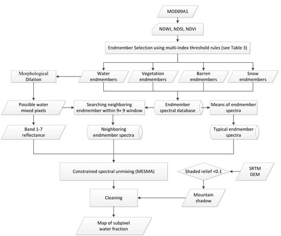
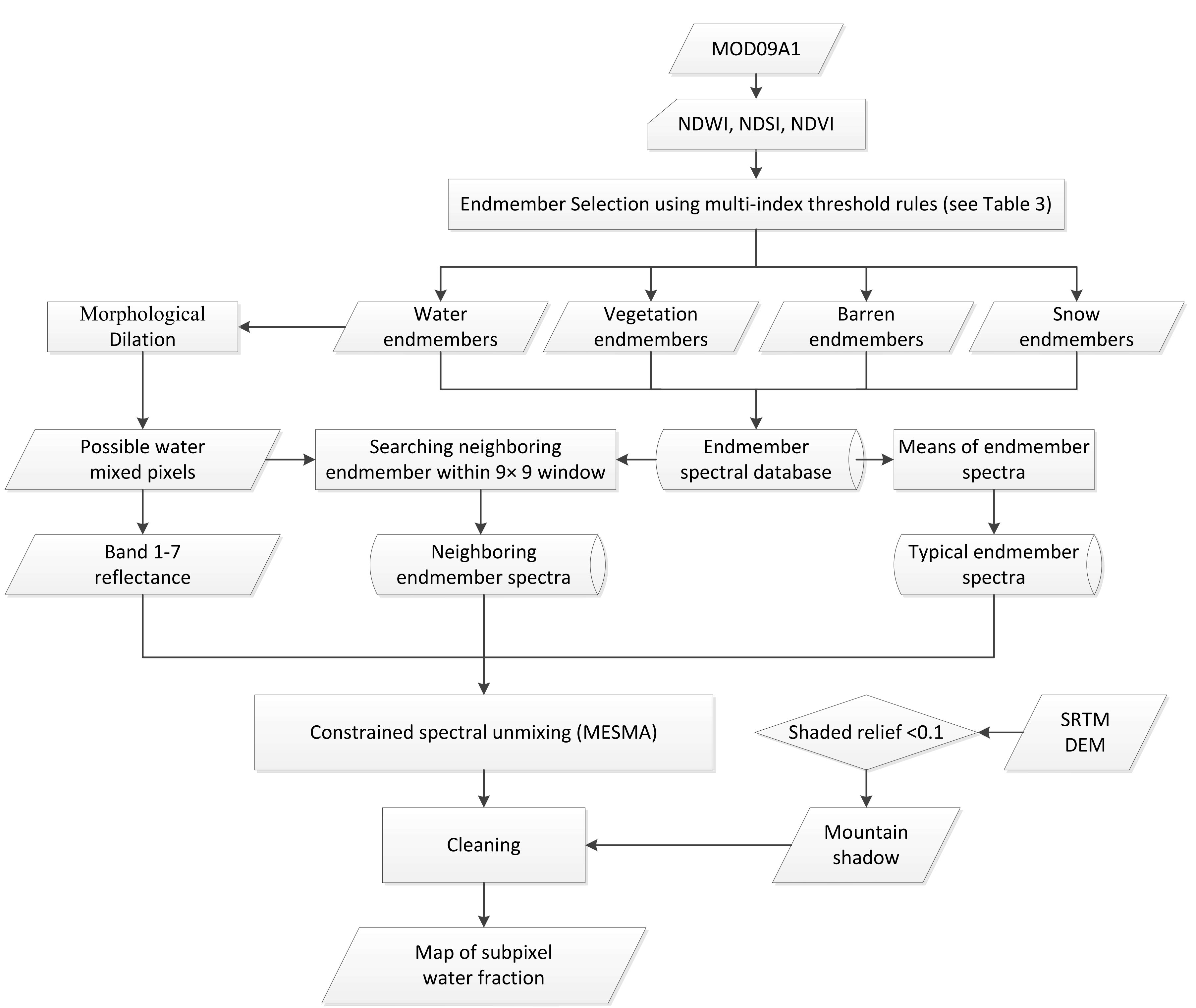
3. Method
3.1. Endmember Selection
3.2. Identification of the Mixed Pixels Contain Water Bodies
3.3. Spectral Mixture Analysis
3.4. Approaches of Using Endmembers in Subpixel Water Mapping
3.5. Cleaning of the Mountain Shadow Area
4. Results
4.1. Validation of the Algorithm with Pairs of OLI/MODIS Images
4.2. Performance of the Water Mapping Algorithm at the Boundary of Water Bodies
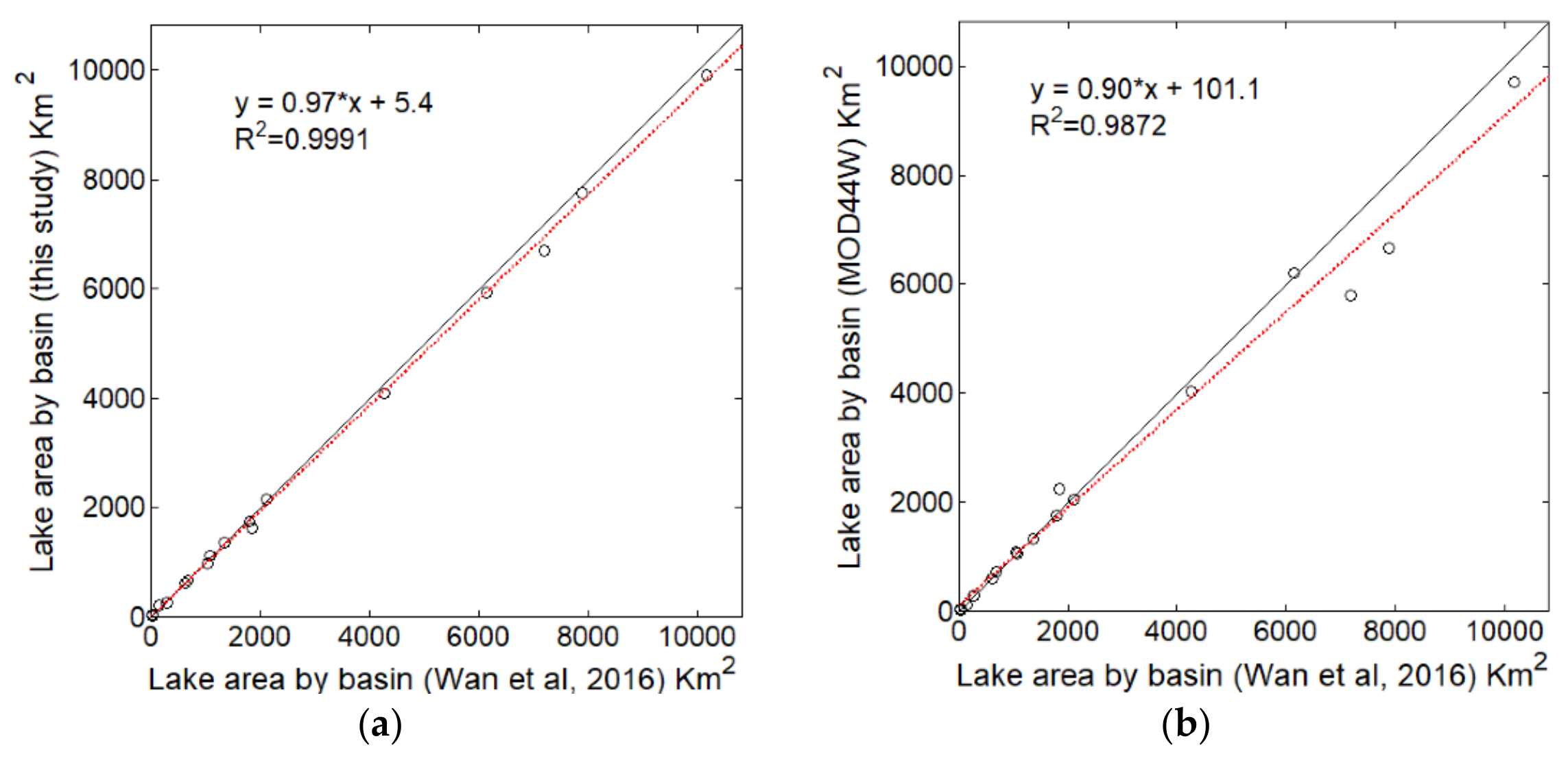
4.3. Validation with the Public Data Sets
5. Discussion
5.1. The Performance of the Endmember Selection Strategy
5.2. Limitations of the Algorithm
5.3. The Potential Implementation of the Proposed Surface Water Unmixing Algorithm
6. Conclusions
Author Contributions
Funding
Acknowledgments
Conflicts of Interest
References
- Qiu, J. China: The third pole. Nat. News 2008, 454, 393–396. [Google Scholar] [CrossRef] [PubMed]
- Yao, T.; Thompson, L.G.; Mosbrugger, V.; Zhang, F.; Ma, Y.; Luo, T.; Xu, B.; Yang, X.; Joswiak, D.R.; Wang, W. Third pole environment (TPE). Environ. Dev. 2012, 3, 52–64. [Google Scholar] [CrossRef]
- Duan, A.; Wu, G. Role of the Tibetan Plateau thermal forcing in the summer climate patterns over subtropical Asia. Clim. Dyn. 2005, 24, 793–807. [Google Scholar] [CrossRef]
- Wu, G.; Liu, Y.; Zhang, Q.; Duan, A.; Wang, T.; Wan, R.; Liu, X.; Li, W.; Wang, Z.; Liang, X. The influence of mechanical and thermal forcing by the Tibetan Plateau on Asian climate. J. Hydrometeorol. 2007, 8, 770–789. [Google Scholar] [CrossRef]
- Yang, K.; Wu, H.; Qin, J.; Lin, C.; Tang, W.; Chen, Y. Recent climate changes over the Tibetan Plateau and their impacts on energy and water cycle: A review. Glob. Planet. Chang. 2014, 112, 79–91. [Google Scholar] [CrossRef]
- Zhang, G.; Xie, H.; Kang, S.; Yi, D.; Ackley, S.F. Monitoring lake level changes on the Tibetan Plateau using ICESat altimetry data (2003–2009). Remote Sens. Environ. 2011, 115, 1733–1742. [Google Scholar] [CrossRef]
- Ogutu-Ohwayo, R.; Hecky, R.E.; Cohen, A.S.; Kaufman, L. Human impacts on the African great lakes. Environ. Biol. Fishes 1997, 50, 117–131. [Google Scholar] [CrossRef]
- Qin, B. Approaches to mechanisms and control of eutrophication of shallow lakes in the middle and lower reaches of the Yangze River. J. Lake Sci. 2002, 14, 193–202. [Google Scholar]
- Wetzel, R.G. Limnology: Lake and River Ecosystems; Gulf Professional Publishing: Houston, TX, USA, 2001. [Google Scholar]
- Yang, K.; Ye, B.; Zhou, D.; Wu, B.; Foken, T.; Qin, J.; Zhou, Z. Response of hydrological cycle to recent climate changes in the Tibetan Plateau. Clim. Chang. 2011, 109, 517–534. [Google Scholar] [CrossRef]
- Lehner, B.; Döll, P. Development and validation of a global database of lakes, reservoirs and wetlands. J. Hydrol. 2004, 296, 1–22. [Google Scholar] [CrossRef]
- Wan, W.; Long, D.; Hong, Y.; Ma, Y.; Yuan, Y.; Xiao, P.; Duan, H.; Han, Z.; Gu, X. A lake data set for the Tibetan Plateau from the 1960s, 2005, and 2014. Sci. Data 2016, 3, 160039. [Google Scholar] [CrossRef] [PubMed]
- Lei, Y.; Yao, T.; Bird, B.W.; Yang, K.; Zhai, J.; Sheng, Y. Coherent lake growth on the central Tibetan Plateau since the 1970s: Characterization and attribution. J. Hydrol. 2013, 483, 61–67. [Google Scholar] [CrossRef]
- Zhang, G.; Xie, H.; Yao, T.; Li, H.; Duan, S. Quantitative water resources assessment of Qinghai Lake basin using Snowmelt Runoff Model (SRM). J. Hydrol. 2014, 519, 976–987. [Google Scholar] [CrossRef]
- Verpoorter, C.; Kutser, T.; Seekell, D.A.; Tranvik, L.J. A global inventory of lakes based on high-resolution satellite imagery. Geophys. Res. Lett. 2014, 41, 6396–6402. [Google Scholar] [CrossRef]
- Verpoorter, C.; Kutser, T.; Tranvik, L. Automated mapping of water bodies using Landsat multispectral data. Limnol. Oceanogr. Methods 2012, 10, 1037–1050. [Google Scholar] [CrossRef]
- White, K.; El Asmar, H.M. Monitoring changing position of coastlines using Thematic Mapper imagery, an example from the Nile Delta. Geomorphology 1999, 29, 93–105. [Google Scholar] [CrossRef]
- Zhang, G.; Zheng, G.; Gao, Y.; Xiang, Y.; Lei, Y.; Li, J. Automated water classification in the Tibetan plateau using Chinese GF-1 WFV data. Photogramm. Eng. Remote Sens. 2017, 83, 509–519. [Google Scholar] [CrossRef]
- Zhang, G.; Yao, T.; Chen, W.; Zheng, G.; Shum, C.K.; Yang, K.; Piao, S.; Sheng, Y.; Yi, S.; Li, J.; et al. Regional differences of lake evolution across China during 1960s–2015 and its natural and anthropogenic causes. Remote Sens. Environ. 2019, 221, 386–404. [Google Scholar] [CrossRef]
- McFeeters, S.K. The use of the Normalized Difference Water Index (NDWI) in the delineation of open water features. Int. J. Remote Sens. 1996, 17, 1425–1432. [Google Scholar] [CrossRef]
- Xu, H. Modification of normalised difference water index (NDWI) to enhance open water features in remotely sensed imagery. Int. J. Remote Sens. 2006, 27, 3025–3033. [Google Scholar] [CrossRef]
- Xie, H.; Luo, X.; Xu, X.; Pan, H.; Tong, X. Automated Subpixel Surface Water Mapping from Heterogeneous Urban Environments Using Landsat 8 OLI Imagery. Remote Sens. 2016, 8, 584. [Google Scholar] [CrossRef]
- Pekel, J.-F.; Cottam, A.; Gorelick, N.; Belward, A.S. High-resolution mapping of global surface water and its long-term changes. Nature 2016, 540, 418. [Google Scholar] [CrossRef] [PubMed]
- Roy, D.P.; Ju, J.; Lewis, P.; Schaaf, C.; Gao, F.; Hansen, M.; Lindquist, E. Multi-temporal MODIS–Landsat data fusion for relative radiometric normalization, gap filling, and prediction of Landsat data. Remote Sens. Environ. 2008, 112, 3112–3130. [Google Scholar] [CrossRef]
- Carroll, M.L.; Townshend, J.R.; DiMiceli, C.M.; Noojipady, P.; Sohlberg, R.A. A new global raster water mask at 250 m resolution. Int. J. Digit. Earth 2009, 2, 291–308. [Google Scholar] [CrossRef]
- Khandelwal, A.; Karpatne, A.; Marlier, M.E.; Kim, J.; Lettenmaier, D.P.; Kumar, V. An approach for global monitoring of surface water extent variations in reservoirs using MODIS data. Remote Sens. Environ. 2017, 202, 113–128. [Google Scholar] [CrossRef]
- Wu, Y.; Li, M.; Guo, L.; Zheng, H.; Zhang, H. Investigating Water Variation of Lakes in Tibetan Plateau Using Remote Sensed Data Over the Past 20 Years. IEEE J. Stars 2019, 12, 2557–2564. [Google Scholar] [CrossRef]
- Sun, F.; Zhao, Y.; Gong, P.; Ma, R.; Dai, Y. Monitoring dynamic changes of global land cover types: Fluctuations of major lakes in China every 8 days during 2000–2010. Chin. Sci. Bull. 2014, 59, 171–189. [Google Scholar] [CrossRef]
- Lu, S.; Jia, L.; Zhang, L.; Wei, Y.; Baig, M.H.A.; Zhai, Z.; Meng, J.; Li, X.; Zhang, G. Lake water surface mapping in the Tibetan Plateau using the MODIS MOD09Q1 product. Remote Sens. Lett. 2017, 8, 224–233. [Google Scholar] [CrossRef]
- Foody, G.M.; Muslim, A.M.; Atkinson, P.M. Super-resolution mapping of the waterline from remotely sensed data. Int. J. Remote Sens. 2005, 26, 5381–5392. [Google Scholar] [CrossRef]
- Dennison, P.E.; Roberts, D.A. Endmember selection for multiple endmember spectral mixture analysis using endmember average RMSE. Remote Sens. Environ. 2003, 87, 123–135. [Google Scholar] [CrossRef]
- Painter, T.H.; Dozier, J.; Roberts, D.A.; Davis, R.E.; Green, R.O. Retrieval of subpixel snow-covered area and grain size from imaging spectrometer data. Remote Sens. Environ. 2003, 85, 64–77. [Google Scholar] [CrossRef]
- Painter, T.H.; Roberts, D.A.; Green, R.O.; Dozier, J. The Effect of Grain Size on Spectral Mixture Analysis of Snow-Covered Area from AVIRIS Data. Remote Sens. Environ. 1998, 65, 320–332. [Google Scholar] [CrossRef]
- Quintano, C.; Fernández-Manso, A.; Roberts, D.A. Multiple Endmember Spectral Mixture Analysis (MESMA) to map burn severity levels from Landsat images in Mediterranean countries. Remote Sens. Environ. 2013, 136, 76–88. [Google Scholar] [CrossRef]
- Roberts, D.A.; Gardner, M.; Church, R.; Ustin, S.; Scheer, G.; Green, R.O. Mapping Chaparral in the Santa Monica Mountains Using Multiple Endmember Spectral Mixture Models. Remote Sens. Environ. 1998, 65, 267–279. [Google Scholar] [CrossRef]
- Ma, R.; Yang, G.; Duan, H.; Jiang, J.; Wang, S.; Feng, X.; Li, A.; Kong, F.; Xue, B.; Wu, J.; et al. China’s lakes at present: Number, area and spatial distribution. Sci. China Earth Sci. 2011, 54, 283–289. [Google Scholar] [CrossRef]
- Immerzeel, W.W.; van Beek, L.P.H.; Bierkens, M.F.P. Climate Change Will Affect the Asian Water Towers. Science 2010, 328, 1382. [Google Scholar] [CrossRef]
- van Zyl, J.J. The Shuttle Radar Topography Mission (SRTM): A breakthrough in remote sensing of topography. Acta Astronaut. 2001, 48, 559–565. [Google Scholar] [CrossRef]
- Valeriano, M.M.; Kuplich, T.M.; Storino, M.; Amaral, B.D.; Mendes, J.N., Jr.; Lima, D.J. Modeling small watersheds in Brazilian Amazonia with shuttle radar topographic mission-90 m data. Comput. Geosci. 2006, 32, 1169–1181. [Google Scholar] [CrossRef]
- Zhang, G.; Yao, T.; Xie, H.; Kang, S.; Lei, Y. Increased mass over the Tibetan Plateau: From lakes or glaciers? Geophys. Res. Lett. 2013, 40, 2125–2130. [Google Scholar] [CrossRef]
- SRTM 90m DEM Digital Elevation Database. Available online: http://srtm.csi.cgiar.org/ (accessed on 3 April 2020).
- NASA’s Earth Observing System Data and Information System. Available online: https://search.earthdata.nasa.gov/search (accessed on 3 April 2020).
- Vermote, E.; Kotchenova, S.; Ray, J. MODIS surface reflectance user’s guide. In MODIS Land Surface Reflectance Science Computing Facility; NASA GSFC: Greenbelt, MD, USA, 2011; Version 1; Volume 1. Available online: https://modis-land.gsfc.nasa.gov/pdf/MOD09_UserGuide_v1.4.pdf (accessed on 3 April 2020).
- US Geological Survey (USGS) website. Available online: https://earthexplorer.usgs.gov/ (accessed on 3 April 2020).
- Zanter, K. Landsat 8 (L8) data users handbook. In Landsat Science Official Website; 2019. Available online: https://www.usgs.gov/land-resources/nli/landsat/landsat-8-data-users-handbook (accessed on 3 April 2020).
- Data_TPLakes. Available online: https://figshare.com/articles/Data_TPLakes/3145369 (accessed on 3 April 2020).
- Carroll, M.L.; DiMiceli, C.M.; Townshend, J.R.G.; Sohlberg, R.A.; Elders, A.I.; Devadiga, S.; Sayer, A.M.; Levy, R.C. Development of an operational land water mask for MODIS Collection 6, and influence on downstream data products. Int. J. Digit. Earth 2017, 10, 207–218. [Google Scholar] [CrossRef]
- Global Lakes and Wetlands Database. Available online: https://www.worldwildlife.org/pages/global-lakes-and-wetlands-database (accessed on 3 April 2020).
- Global Surface Water - Data Access. Available online: https://global-surface-water.appspot.com/download (accessed on 3 April 2020).
- Elmore, A.J.; Mustard, J.F.; Manning, S.J.; Lobell, D.B. Quantifying Vegetation Change in Semiarid Environments: Precision and Accuracy of Spectral Mixture Analysis and the Normalized Difference Vegetation Index. Remote Sens. Environ. 2000, 73, 87–102. [Google Scholar] [CrossRef]
- Adams, J.B.; Sabol, D.E.; Kapos, V.; Almeida Filho, R.; Roberts, D.A.; Smith, M.O.; Gillespie, A.R. Classification of multispectral images based on fractions of endmembers: Application to land-cover change in the Brazilian Amazon. Remote Sens. Environ. 1995, 52, 137–154. [Google Scholar] [CrossRef]
- Atkinson, P.; Cutler, M.; Lewis, H. Mapping sub-pixel proportional land cover with AVHRR imagery. Int. J. Remote Sens. 1997, 18, 917–935. [Google Scholar] [CrossRef]
- Song, C. Spectral mixture analysis for subpixel vegetation fractions in the urban environment: How to incorporate endmember variability? Remote Sens. Environ. 2005, 95, 248–263. [Google Scholar] [CrossRef]
- Van der Meer, F.D.; Jia, X. Collinearity and orthogonality of endmembers in linear spectral unmixing. Int. J. Appl. Earth Obs. Geoinf. 2012, 18, 491–503. [Google Scholar] [CrossRef]
- Chenzhou, L.; Donghui, X.; Shi, J.; Shuai, G. Subpixel mapping of water cover with MODIS in Tibetan Plateau. In Proceedings of the Geoscience and Remote Sensing Symposium (IGARSS 2009), Cape Town, South Africa, 12–17 July 2009; pp. IV-307–IV-309. [Google Scholar]
- Shi, J. An automatic algorithm on estimating sub-pixel snow cover from MODIS. Quatemary Sci. 2012, 32, 6–15. [Google Scholar]
- Zhu, J.; Shi, J.; Wang, Y. Subpixel snow mapping of the Qinghai–Tibet Plateau using MODIS data. Int. J. Appl. Earth Obs. Geoinf. 2012, 18, 251–262. [Google Scholar] [CrossRef]
- Dozier, J. Spectral signature of alpine snow cover from the landsat thematic mapper. Remote Sens. Environ. 1989, 28, 9–22. [Google Scholar] [CrossRef]
- Rouse, J.W., Jr.; Haas, R.; Schell, J.; Deering, D. Monitoring vegetation systems in the Great Plains with ERTS. NASA Spec. Publ. 1974, 351, 309. [Google Scholar]
- Sabol, D.E., Jr.; Adams, J.B.; Smith, M.O. Quantitative subpixel spectral detection of targets in multispectral images. J. Geophys. Res. Planets 1992, 97, 2659–2672. [Google Scholar] [CrossRef]
- Somers, B.; Asner, G.P.; Tits, L.; Coppin, P. Endmember variability in Spectral Mixture Analysis: A review. Remote Sens. Environ. 2011, 115, 1603–1616. [Google Scholar] [CrossRef]
- Deng, C.; Wu, C. A spatially adaptive spectral mixture analysis for mapping subpixel urban impervious surface distribution. Remote Sens. Environ. 2013, 133, 62–70. [Google Scholar] [CrossRef]
- Gao, F.; Hilker, T.; Zhu, X.; Anderson, M.; Masek, J.; Wang, P.; Yang, Y. Fusing Landsat and MODIS Data for Vegetation Monitoring. IEEE Geosci. Remote Sens. Mag. 2015, 3, 47–60. [Google Scholar] [CrossRef]
- Vermote, E.; Justice, C.; Claverie, M.; Franch, B. Preliminary analysis of the performance of the Landsat 8/OLI land surface reflectance product. Remote Sens. Environ. 2016, 185, 46–56. [Google Scholar] [CrossRef]
- Shi, K.; Zhang, Y.; Zhu, G.; Liu, X.; Zhou, Y.; Xu, H.; Qin, B.; Liu, G.; Li, Y. Long-term remote monitoring of total suspended matter concentration in Lake Taihu using 250 m MODIS-Aqua data. Remote Sens. Environ. 2015, 164, 43–56. [Google Scholar] [CrossRef]
- Miller, R.L.; McKee, B.A. Using MODIS Terra 250 m imagery to map concentrations of total suspended matter in coastal waters. Remote Sens. Environ. 2004, 93, 259–266. [Google Scholar] [CrossRef]
- Dorji, P.; Fearns, P.; Broomhall, M. A Semi-Analytic Model for Estimating Total Suspended Sediment Concentration in Turbid Coastal Waters of Northern Western Australia Using MODIS-Aqua 250 m Data. Remote Sens. 2016, 8, 556. [Google Scholar] [CrossRef]


| Image NO | Landsat 8 OLI | MODIS | Cover Lakes | |||
|---|---|---|---|---|---|---|
| Acquisition date | DOY | WRS Path | WRS Row | DOY | ||
| 1 | 13/11/2014 | 317 | 133 | 34 | 313–320 | Qinghai Lake |
| 2 | 7/11/2014 | 311 | 139 | 38 | 305–312 | Selin Co |
| 3 | 15/10/2014 | 288 | 138 | 39 | 281–288 | Nam Co |
| 4 | 26/08/2014 | 238 | 140 | 34 | 233–240 | Ayakkum Lake |
| 5 | 31/07/2013 | 212 | 139 | 36 | 209–216 | Wulanwula Lake |
| 6 | 7/10/2013 | 280 | 135 | 33 | 273–280 | Har Lake |
| 7 | 11/06/2013 | 162 | 141 | 39 | 161–168 | Zhari Namco |
| 8 | 19/11/2014 | 323 | 143 | 38 | 321–328 | Ngangla Ringco |
| Index | Equation | Remark | Reference |
|---|---|---|---|
| Normalized Difference Water Index | NDWI = (B4 − B2)/(B4 + B2) | Water has positive value | [20] |
| Normalized Difference Snow Index | NDSI = (B4 − B6)/(B4 + B6) | Snow has a greater value | [58] |
| Normalized Difference Vegetation Index | NDVI = (B2 − B1)/(B2 + B1) | Vegetation has a greater value | [59] |
| Endmember Class | Rules |
|---|---|
| Water | NDWI > 0.1 and B2 < 0.2 |
| Snow | NDVI < −0.035 and NDSI > 0.75 and B4 > 0.7 |
| Vegetation | NDVI > 0.7 and NDSI < −0.4 |
| Barren | NDVI > 0 and NDVI < 0.15 and NDSI < −0.4 |
| Image No. | Water Area (103 km2) | Error (%) | RMSE (%) | Bias (%) | R2 | Linear regression | ||||
|---|---|---|---|---|---|---|---|---|---|---|
| OLI | MOD | M500 | G1000 | M500 | G1000 | M500 | G1000 | |||
| G2000 | G2000 | G2000 | ||||||||
| 1 | 4.397 | 4.359 | −0.87 | 8.6 | 6.8 | −0.3 | 0.96 | 0.98 | y = 0.97x + 0.005 | y = 0.98x + 0.003 |
| 4.8 | 0.99 | y = 0.99x + 0.001 | ||||||||
| 2 | 3.815 | 3.629 | −4.87 | 10.1 | 7.7 | −0.9 | 0.93 | 0.96 | y = 0.94x + 0.002 | y = 0.96x − 0.001 |
| 5.4 | 0.98 | y = 0.97x − 0.003 | ||||||||
| 3 | 2.064 | 2.015 | −2.38 | 7.5 | 5.6 | −0.6 | 0.97 | 0.98 | y = 0.97x + 0.001 | y = 0.98x − 0.001 |
| 3.8 | 0.99 | y = 0.99x − 0.003 | ||||||||
| 4 | 0.966 | 1.001 | 3.59 | 4.2 | 3.2 | 0.3 | 0.98 | 0.99 | y = x + 0.003 | y = x + 0.002 |
| 2.3 | 0.99 | y = x + 0.002 | ||||||||
| 5 | 0.655 | 0.648 | −1.01 | 8.4 | 5.8 | −0.2 | 0.95 | 0.97 | y = 0.97x + 0.004 | y = 0.99x + 0.001 |
| 3.6 | 0.99 | y = x − 0.001 | ||||||||
| 6 | 0.590 | 0.615 | 4.15 | 4.4 | 3.4 | 0.3 | 0.97 | 0.98 | y = x + 0.003 | y = x + 0.003 |
| 2.5 | 0.99 | y = x + 0.002 | ||||||||
| 7 | 1.088 | 1.099 | 0.94 | 5.8 | 4.1 | 0.1 | 0.97 | 0.98 | y = 0.98x + 0.004 | y = 0.99x + 0.002 |
| 2.7 | 0.99 | y = x + 0.002 | ||||||||
| 8 | 0.684 | 0.694 | 1.43 | 8.0 | 5.8 | 0.1 | 0.94 | 0.98 | y = 0.97x + 0.006 | y = 0.98x + 0.004 |
| 3.9 | 0.99 | y = 0.99x + 0.003 | ||||||||
| Overall | 14.259 | 14.06 | −1.40 | 7.86 | 6.0 | −0.2 | 0.96 | 0.98 | y = 0.97x + 0.003 | y = 0.98x + 0.001 |
| 4.1 | 0.99 | y = 0.99x − 0.0002 | ||||||||
| MOD09A1 | Landsat 8 OLI | ||
|---|---|---|---|
| band | bandwidth (μm) | band | bandwidth (μm) |
| 1 | 0.620–0.670 | 4 | 0.636–0.673 |
| 2 | 0.841–0.876 | 5 | 0.851–0.879 |
| 3 | 0.459–0.479 | 2 | 0.452–0.512 |
| 4 | 0.545–0.565 | 3 | 0.533–0.590 |
| 6 | 1.628–1.652 | 6 | 1.566–1.651 |
| 7 | 2.105–2.155 | 7 | 2.107–2.294 |
| Basin | Lake Area (km2) | Area Difference* (km2) | Area Difference* (%) | |||||||
|---|---|---|---|---|---|---|---|---|---|---|
| This Study | MOD44W | ESA | Wan et al. (2016) | This Study | MOD44W | ESA | This Study | MOD44W | ESA | |
| AmuDarya | 653.17 | 710.74 | 680.41 | 673.03 | −19.86 | 37.71 | −62.26 | −2.95 | 5.6 | 1.10 |
| Brahmaputra | 1624.35 | 2237.21 | 1887.29 | 1839.26 | −214.91 | 397.95 | 4.12 | −11.68 | 21.64 | 2.61 |
| Ganges | 42.07 | 24.55 | 20.41 | 20.6 | 21.47 | 3.95 | 9.12 | 104.23 | 19.15 | −0.92 |
| Hexi | 612.49 | 602.94 | 603.95 | 615.13 | −2.64 | −12.19 | −19.11 | −0.43 | −1.98 | −1.82 |
| Z`Indus | 1733.83 | 1759.57 | 1775.7 | 1791.08 | −57.25 | −31.51 | −8.81 | −3.2 | −1.76 | −0.86 |
| Inner A | 9920.34 | 9710.88 | 10,263.75 | 10,172.96 | −252.62 | −462.08 | −38.51 | −2.48 | −4.54 | 0.89 |
| Inner B | 4095.13 | 4035.24 | 4199.43 | 4263.94 | −168.81 | −228.7 | 7.64 | −3.96 | −5.36 | −1.51 |
| Inner C | 1351.84 | 1323.78 | 1363.68 | 1342.63 | 9.21 | −18.85 | −14.24 | 0.69 | −1.4 | 1.57 |
| Inner D | 2151.97 | 2032.96 | 2097.34 | 2111.58 | 40.39 | −78.62 | 21.05 | 1.91 | −3.72 | −0.67 |
| Inner E | 6705.66 | 5795.78 | 7187.28 | 7179.64 | −473.98 | −1383.86 | −64.51 | −6.6 | −19.27 | 0.11 |
| Inner F | 7755.59 | 6665.55 | 7850.97 | 7889.48 | −133.89 | −1223.93 | 90.79 | −1.7 | −15.51 | −0.49 |
| Mekong | 7.81 | 14.66 | 8.72 | 17.53 | −9.72 | −2.87 | −15.38 | −55.43 | −16.36 | −50.26 |
| Qaidam | 1109.41 | 1051.31 | 1050.04 | 1069.15 | 40.26 | −17.84 | −11.18 | 3.77 | −1.67 | −1.79 |
| Salween | 250.65 | 280.74 | 285.11 | 275.99 | −25.34 | 4.75 | −0.19 | −9.18 | 1.72 | 3.31 |
| Tarim | 208.74 | 106.29 | 153.03 | 148.91 | 59.83 | −42.62 | 48.03 | 40.18 | −28.62 | 2.77 |
| Yangtze | 960.05 | 1069.68 | 1042.44 | 1040.28 | −80.23 | 29.4 | 7.38 | −7.71 | 2.83 | 0.21 |
| Yellow | 5941.94 | 6194.84 | 6081.63 | 6143.89 | −201.95 | 50.95 | 2.16 | −3.29 | 0.83 | −1.01 |
| TP total | 45,125.04 | 43,616.72 | 46,551.18 | 46,595.08 | −1470.04 | −2978.36 | −43.90 | −3.15 | −6.39 | −0.09 |
© 2020 by the authors. Licensee MDPI, Basel, Switzerland. This article is an open access article distributed under the terms and conditions of the Creative Commons Attribution (CC BY) license (http://creativecommons.org/licenses/by/4.0/).
Share and Cite
Liu, C.; Shi, J.; Liu, X.; Shi, Z.; Zhu, J. Subpixel Mapping of Surface Water in the Tibetan Plateau with MODIS Data. Remote Sens. 2020, 12, 1154. https://doi.org/10.3390/rs12071154
Liu C, Shi J, Liu X, Shi Z, Zhu J. Subpixel Mapping of Surface Water in the Tibetan Plateau with MODIS Data. Remote Sensing. 2020; 12(7):1154. https://doi.org/10.3390/rs12071154
Chicago/Turabian StyleLiu, Chenzhou, Jiancheng Shi, Xiuying Liu, Zhaoyong Shi, and Ji Zhu. 2020. "Subpixel Mapping of Surface Water in the Tibetan Plateau with MODIS Data" Remote Sensing 12, no. 7: 1154. https://doi.org/10.3390/rs12071154
APA StyleLiu, C., Shi, J., Liu, X., Shi, Z., & Zhu, J. (2020). Subpixel Mapping of Surface Water in the Tibetan Plateau with MODIS Data. Remote Sensing, 12(7), 1154. https://doi.org/10.3390/rs12071154