Abstract
With knowledge of geometry and density-distribution of topography, the residual terrain modelling (RTM) technique has been broadly applied in geodesy and geophysics for the determination of the high-frequency gravity field signals. Depending on the size of investigation areas, challenges in computational efficiency are encountered when using an ultra-high-resolution digital elevation model (DEM) in the Newtonian integration. For efficient and accurate gravity forward modelling in the spatial domain, we developed a new MATLAB-based program called, terrain gravity field (TGF). Our new software is capable of calculating the gravity field generated by an arbitrary topographic mass-density distribution. Depending on the attenuation character of gravity field with distance, the adaptive algorithm divides the integration masses into four zones, and adaptively combines four types of geometries (i.e., polyhedron, prism, tesseroid and point-mass) and DEMs with different spatial resolutions. Compared to some publicly available algorithms depending on one type of geometric approximation, this enables accurate modelling of gravity field and greatly reduces the computation time. Besides, the TGF software allows to calculate ten independent gravity field functionals, supports two types of density inputs (constant density value and digital density map), and considers the curvature of the Earth by involving spherical approximation and ellipsoidal approximation. Further to this, the TGF software is also capable of delivering the gravity field of full-scale topographic gravity field implied by masses between the Earth’s surface and mean sea level. In this contribution, the TGF software is introduced to the geoscience community and its capabilities are explained. Results from internal and external numerical validation experiments of TGF confirmed its accuracy at the sub-mGal level. Based on TGF, the trade-off between accuracy and efficiency, values for the spatial resolution and extension of topography models are recommended. The TGF software has been extensively tested and recently been applied in the SRTM2gravity project to convert the global 3” SRTM topography to implied gravity effects at 28 billion computation points. This confirms the capability of TGF for dealing with large datasets. Together with this paper, the TGF software will be released in the public domain for free use in geodetic and geophysical forward modelling computations.
1. Introduction
The gravitational field, including the gravitational potential and its first and second derivatives, is one of the Earth’s fundamental properties. It provides insights into the mass-density distributions, such as inner structures and subsurface density variations. The topographic gravity field is the field contribution generated by Earth’s topographic masses and is computed using gravity forward modelling techniques (e.g., [1]). The topographic gravity field plays an essential role in geodesy and geophysics applications, e.g., smoothing gravity observation in the remove-compute-restore procedure [2,3], reduction of the gravity observations in boundary-value problem [4,5], for prediction of high-frequency gravity field constituents [6,7,8], and for the reduction of omission errors in height system definitions and unification [9].
In the last few decades, considerable attention has been given to the forward modelling approaches, either in the spectral domain through spherical harmonic analysis (SHA) of height-density functions (globally, e.g., [10,11,12]; regionally, e.g., [13]) and spherical harmonic synthesis (SHS) for computation points, or in the spatial domain using analytical or numerical gravitational formulas of geometries. In the spectral domain, the evaluation of gravitational field relies on the spherical harmonic expansions of powers of the topography. The classical libraries such as SHTOOLS [14] permit to expand a given field up to spherical harmonic degree 2,800, and ultra-high resolution (e.g., 10,800 and beyond) SHA based on Fast Fourier Transform (FFT) together with quadrature technique by Rexer and Hirt [15]. The spectral gravity modeling (SGM) technique shows great efficiency in the long-/medium-wavelength global gravity field studies where gravitational potential is modelled through different mass layers, such as in the development of layer-based topographical gravitational field dV_ELL_EARTH2014 [16] and RWI_TOPO_2015 [17] up to degree and order of 2,160, dV_ELL_EARTH2014_5480 [12,18] up to degree of 5480, and the most up-to-date Rock-Ocean-Lake-Ice (ROLI) Topographic Gravity Field Model to degree of 3660 [19]. Due to their lack of detailed resolution, such approaches and models, however, are not optimal for local applications demanding high-resolution gravity knowledge such as reduction of gravity-related observations, hydrological mass transports and redistribution, and inertial navigation. A viable, well-known and frequently used approach is gravity forward modelling through Newtonian integration (NI) in the spatial domain.
The topography generally has a complex geometric structure, which makes a general analytical solution of Newton’s integral for an arbitrary-shaped body impossible. Therefore, the discretization and approximation with primitive mass-elements (e.g., prism or tesseroid) mimicking the shape of the mass sources with a series of regular geometries [20] is common practice. The composite gravitational field is then obtained by summing up the effects of all mass-elements around the evaluation point located on or above the Earth’s surface.
As primitive mass-elements, usually polyhedra, prisms, tesseroids and point-masses are adopted to model and approximate the mass-density distributions. Based on different regularization techniques, a variety of studies and algorithms were implemented and developed over past decades, e.g., the “TC” program for NI with flat-topped prism as mass elementary [6], FFT terrain correction program “tcfour” [6], “tcq” algorithm with Gaussian quadrature [21], C programming “Tesseroids” combining Gauss-Legendre Quadrature (GLQ) with tesseroid-based discretization and regularization [22], “POLYHEDRON” for analytical computation of gravitational field of arbitrary shaped polyhedra [23]. In theory, high-resolution DEMs together with complex geometries, e.g., as represented through a set of polyhedrons, yield a better and more accurate terrain representation, but at the expense of numerical efficiency [24]. In order to achieve the trade-off between accuracy and efficiency, the MATLAB tool GTeC [25] combines three types of geometries (flat-topped square prism, triangle prism and polyhedron) and DEMs with various resolutions within different integration zones. Besides, the efficiency was improved by the parallel computing functions and from the vectorization code. However, the GTeC is limited to the calculation of gravity anomalies of terrain correction and Bouguer effect.
Therefore, to the best of our knowledge there is no gravity forward modelling software code freely available that (1) combines different types of elementary mass-elements especially the more efficient tesseroid and point-mass, while (2) offering the option to calculate various gravity field functionals in (3) different spectral band-widths, including high-frequency gravity modelling (known as residual terrain modelling or RTM) and full-banded modelling where a full topographic mass-model is used as input, (4) with coding made in MATLAB, allowing rather easy modification and adaption of the code for scientific studies. In order to fill this gap, we have developed the new terrain gravity field (TGF) calculation software, which combines four regularization methods: polyhedron, prism, and the more efficient tesseroid and point-mass in form of a readily-usable MATLAB code. The software facilitates the use of various combinations of zone-radius, DEM resolution levels, regularization geometry, and allows calculation of various gravitational field functionals in different spectral bands
The TGF software enables to calculate topography implied gravitational field, including functionals of geoid height, gravity anomaly and all components of the gravity gradient tensor. The TGF software is expected to be beneficial to geodesy and geophysics for scientific tasks related to geometry, gravity field and geological structure of the planet. The topography-implied geoid heights are potentially used to refine the global geoid height model and achieved an accuracy of cm-level [26]. This could be extensively applied in the unification of national height systems on a global scale in order to reduce omission errors of global gravity field models significantly, and transformation of Global Positioning System (GPS) measured geodetic height to physical orthometric height. Besides, topography is one of the main contributors to gravity anomalies. In geophysical studies, the topographic gravity effects are usually reduced before interpretation and modelling of sub-surface structures. Further to the above, the TGF software allows for the calculation of gravity gradients, which contain higher frequency information than gravity anomalies and therefore allow a better localization of mass anomalies. Therefore, this software can be of interest to geophysicists who are interested in modelling lateral density variation of lithospheric structures [27,28].
The goal of this paper is to introduce the new software TGF for gravitational field forward modelling calculations. We briefly outline theoretical aspects of gravity forward modelling in the spatial domain (Section 2), then introduce the software design, structure and workflow in Section 3, and present results from external and internal evaluations of topographic and RTM gravity field calculations (Section 4). Based on the investigations on the trade-off between accuracy and numerical efficiency, suitable parameters are recommended allowing accurate yet efficient RTM computations (Section 4). Some conclusions are given in Section 5.
2. Forward Modelling in Space Domain
The gravitational potential caused by a general mass-density distribution at computation point located on or above the Earth’s surface is expressed by Newton’s gravitational integral:
with denoting the universal gravitational constant, being the Euclidean distance between evaluation point and the topographic mass element , indicating the volume’s density over the mass element , and representing the infinitesimal volume element.
In practice, no analytical solution exists for Equation (1) for general mass distributions with arbitrary shape. Instead, the geometry is divided into a model of mesh which can be arbitrarily synchronized to the grid of the available geometrical data (DEMs) and physical parameters (mass density model) (Figure 1a). Analytical or numerical integration schemes are used to evaluate the Newton’s integral, and its first and second derivatives, over each regular volume element. The composite gravity effect over calculation point is then obtained through the summation of all individual contributions.
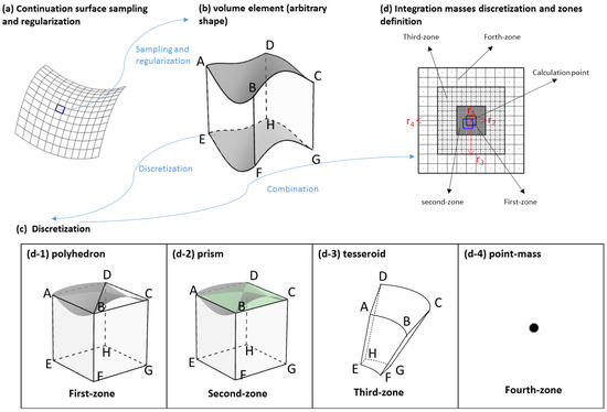
Figure 1.
Discretization and regularization of the mass-distributions.
While the gravitational field attenuates with increasing distance from the evaluation point, the masses in the vicinity of the computation point play a crucial role in the forward modelling procedure, especially for the first and second derivatives of gravitational potential. In order to achieve high accuracy and efficiency, in the TGF software, the mass distributions are divided into four zones (Figure 1c). Polyhedron, prism, tesseroid and point-mass (Figure 1d) are optionally combined by definition of radius of four zones respectively, e.g., using high-resolution DEM and density model together with high-accurate regularization method (e.g., polyhedron or prism) in the closest neighbourhood, using coarse DEM and density map with efficient geometries (e.g., tesseroid or point-mass) in the distant zones.
In the closest zone, mass-distributions cover a square area around the computation point and extend to the distance of from elevation point (Figure 1b). The mass-distributions, located in the closest zone, are discretized and regularized with highly accurate polyhedra. The polyhedra, as shown in Figure 1(d-1), is composed of five square faces and two inclined triangle tops, with their corners coinciding with the grid nodes (cell-center) of the applied DEM (Figure 2), and horizontal sides are equal to the DEM grid resolution. The tops are defined by the ‘DetailedDEM’ used as input (Figure 3), their heights at the top corners (‘A’, ‘B’, ‘C ‘and ‘D’ in Figure 1(d-1)) sharing the elevation values over respective grid centers of ‘DetailedDEM’, while the lower square face (‘EFGH’ in Figure 1(d-1)) is defined by ‘DetailedREF’ (Figure 3) and holds the average height of lower boundary-grid nodes at ‘E’, ’F’, ’G’, and ‘H’. It is worth noting that, with former polyhedron definition, there might exist special cases as shown in Figure 4 where the tops’ corners are located on the different sides of the bottom surface. This means that tops and lower square face meet in a line. Non-analytical solution exists for Newton’s integral of such geometries. In the TGF software, such cases are automatically detected depending on the relations among points and planes. Involving a surface of constant height −1000 m, each irregular geometry was divided into two polyhedrons: (1) one was bounded by the top surface (detailed DEM) and the constant surface (−1000 m), (2) another was defined by the bottom surface (reference DEM) and the constant surface. The potential over the arbitrary geometry is obtained by the difference of these two regular geometries.
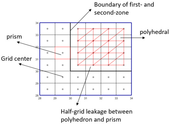
Figure 2.
Leakage problem between polyhedron-zone and prism-zone.
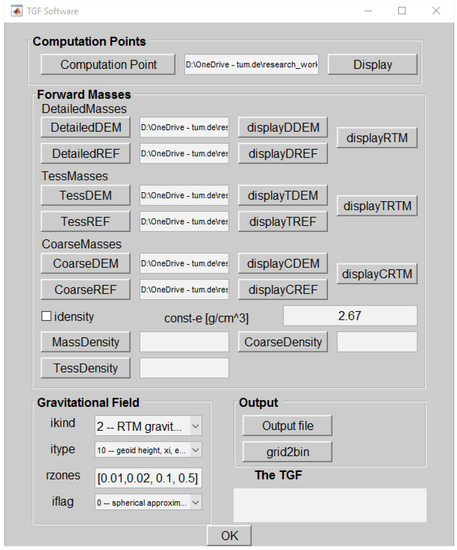
Figure 3.
The Graphical User Interface (GUI) of the terrain gravity field (TGF) software.
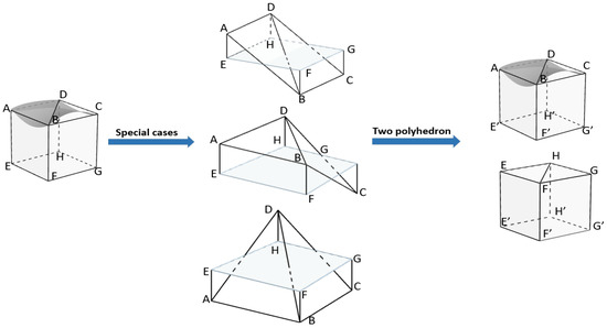
Figure 4.
Special cases for polyhedron.
For Newton’s integral solution of polyhedron, the Fortan code ‘polyhedron.f’ by Tsoulis [23] is applied and combined with our MATLAB software via a so-called MEX-function. With the MEX-function, the corresponding .mex file is necessary for running FORTRAN code in the MATLAB-based TGF software. In the software package, we have built the mex-file .mexa64 for Linux (64-bit), and .mexw64 for Windows (64-bit). For other systems, mex-setup, select the default outline complier and build .mex file are required beforehand. In such cases, a compatible outline FORTRAN compiler for MATLAB is necessary, please refer to the https://de.mathworks.com/support/compilers.html for supported compilers by MathWorks products. If there are multiple versions of compilers, use ‘mex –setup FORTRAN’ to select and change the default compiler for building FORTRAN compiler.
The second zone extends up to distance of from calculation point, which shares the same DEM grid with the closest zone but using flat-topped prism for regularization. The flat-topped prism (Figure 1(d-2)) located at the center of each grid, with lateral and vertical sides corresponding, respectively, to the grid size and to vertical radius. The analytical solutions of flat-topped prism potential and its derivatives are coded as described in [29] and [30]. The Earth’s curvature and effect of plumblines’ convergence are fully taken care of by adopting the methodology of transforming between the prism-based and computation point-based north-oriented local Cartesian coordinate systems [31]. As a consequence of using polyhedral with DEM grid center as corners and the prism centers coinciding with grid center, there occurs a square–circle leakage of half DEM resolution between prism zone and polyhedron zone shown in Figure 2 denoting the adjacent zone (blue outlined square in Figure 1c) between prism and polyhedron. To minimize the leakage, these masses are separately evaluated using tailored prisms.
In the third zone, tesseroids are adopted for regularization. The tesseroid (Figure 1(d-3)) is composed of three pairs of surfaces bounded by a pair of longitudes, a pair of latitudes, and a pair of radii as boundaries. Since there is no analytical solution for tesseroid integrals, the numerical evaluation by expanding the integral kernel to a third-order Taylor series is applied in the TGF software [32]. In this software, no special effort (like subdivision) was made for tesseroid integration of adjacent masses. Therefore, to avoid numerical problems, the tesseroid representation is not recommended for masses integration of the very near zones around the computation point, instead the polyhedron representation is to be preferred.
In the fourth zone, tesseroids are replaced by point-mass (Figure 1(d-4)) of the same mass. In this method, each mass-element in the fourth zone is approximated by a point-mass. The point-mass is located in the mass-center of mass-element. Depending on the attenuation character of gravity with increasing distance, point-mass together with a coarse DEM grid are used for efficient forward modelling of distant masses. The numerical evaluation of point-mass is more than ten times faster than the numerical evaluation of polyhedral and prism [33].
The TGF software distinguishes between forward modelling with a full topographic mass model and with a residual topographic masses model, also known as residual terrain modelling (RTM, [6]). The definition of extensions of each zone will be further investigated in Section 4.3.
Accurate gravity forward modelling in the spatial domain requires integration over the domain of all mass-sources, which often extend to the entire globe for the full-scale gravity field calculation and up to tens of kilometers for RTM gravity field application. Considering the curvature of the Earth, in such cases, the often used local planar approximation is usually not sufficient for the accurate computations. The TGF software therefore adopts the more rigorous spherical or ellipsoidal approximation levels. In the ellipsoidal approximation, the Earth is approximated by a spheroid with a latitude-dependent Earth radius. The relevant coordinates are, ellipsoidal height and geodetic latitude and longitude . All forward computations model the topographic masses relative to the surface of GRS80 ellipsoid. In spherical approximation, Newtonian integration treats the topographic relative to a reference sphere, with GRS80 semi-major axis as radius, and the spherical latitudes, longitudes and heights as coordinate basis.
As for the RTM technique, in some cases calculation points can be located below the reference surface and buried in the mass-distributions. For these points, the direct forward modelling yields the non-harmonic gravitational potential and does therefore not anymore correspond to values observed in harmonic condition, such as observations in the boundary value problem (cf. [34]). It is well-known that some kind of a harmonic correction is required for these points [2]. The mass condensation technique, which has been implemented in the widely-used TC software [6], has been adopted in the TGF software as harmonic correction for RTM gravity calculations, applied for points located inside the reference topography. Following Forsberg [6], this technique condenses the mass layer between the computation point and the reference surface into an infinitesimal thick mass layer immediately below the computation point via,
where is the height difference between the DEM and reference height of the calculation point, is Bouguer density of 2670 kg/m3. Equation (2) is automatically applied by the TGF software for the gravity computations based on the RTM technique.
3. TGF: Structures and Functions
The TGF software works in two modes: in interactive mode with Graphical User Interface (GUI) interface and in batch mode without the GUI interface.
Running in GUI interface: Figure 3 shows the working interface of TGF software. It is divided into four parts, comprising the input of computation points, definition of the mass distributions, specification to the functionals and computation zones, output files.
The computation point information is located and read in the ’Computation Points’ panel. The computation file is defined in binary format with vector for —point number, latitude, longitude and height respectively. The coordinates should be consistent with those of the reference model, e.g., geodetic latitude and ellipsoidal height when referring to an ellipsoid, spherical latitude and orthometric height when using sphere of radius R as reference model.
The ’Forward Mass’ module defines the input file to define the topographic masses, via the geometric upper and lower boundaries and density values. For practical computations, the mass distributions are divided into four zones and defined by three sets of DEM and density inputs, where resolutions varying with zone-distance from computation point. A detailed DEM (pushbuttons—‘DetailedDEM’, ‘DetailedREF’ for RTM computation) defines the masses for polyhedron and prism. ’TessMasses’ with ’TESSDEM’, ’TESSREF’ and ’TessDensity’ defines the tesseroid applied zone, and a coarse DEM (pushbuttons—‘CoarseDEM’, ‘CoarseREF’ for RTM computation) are required for point-mass modeling. Through choosing the respective ’displayed’ button, all DEM can be imaged and displayed for pre-access. ‘displayRTM’ and ‘displayCRTM’ show the height differences between Earth surface and its smooth reference surface. It works only when RTM gravitational field has been selected. The checkbox ‘idensity’ represents the flag for mass-density, 0 for constant density, 1 for various density map. A density map, e.g., CRUST 1.0 [35] and New Zealand digital density map [36], is used and required when ‘various density’ is selected, otherwise a constant mass-density value as the most common case. Density unit in all cases is . Elevation data is in binary format of vector ‘[minphi manphi resphi minlam maxlam reslam elevation]’, minimum, maximum and resolution of DEM grid latitude, minimum, maximum and resolution of DEM grid longitude, and DEM height. Similarly, mass density models are of format in vector ‘[minphi manphi resphi minlam maxlam reslam density]’.
In the module ‘Gravitational Field’, as listed in the Table 1, ‘ikind’ defines the potential type with values of 1 for the topographic gravitational field, and 2 for RTM gravitational field. ‘itype’ defines required computation functions with values of 0 for height anomaly/geoid height (), 1 of vertical deflections (VD) () and gravity disturbances (), 4 of vertical deflections and gravity anomaly (), 2 for gravity tensors, 10 for ten elements (geoid, gravity disturbance, vertical deflections and five independent components of gradient tensor, 103 for geoid height, vertical deflection and gravity disturbance, and 104 for geoid, vertical deflections and gravity anomaly. The formulas are shown in Equations (3)–(8) with indicating the vertical radius and representing normal gravity at calculation point with latitude and longitude . The triple defines the coordinates of calculation point in the local north-oriented coordinate system, ‘rzones’ defines the extension of each zone in degree. As demonstrated in Section 2, prism or polyhedron is suggested in the very near zone (e.g., 0.03° from calculation point) to avoid unacceptably large errors. A larger radius of integration zones generally increases the computational load and memory demand. ‘iflag’ defines the reference model, with ‘0’ when referring to a sphere of radius of , and ‘1’ when referring to an ellipsoid (WGS84 parameters are adopted in the TGF software).

Table 1.
Parameter specification for TGF forward modeling.
The publicly available DEM datasets are generally prepared with tiles that contain a matrix of elevation values arranged at a regularly spaced grid in geographic latitude and longitude, such as SRTM DEMs. By pressing the pushbutton ‘grid2bin’, the interface ‘grid2bin’ (Figure 5) is displayed and helps converting such grid file to binary format which could be recognized by TGF software. The ‘grid2bin’ interface allows the definition of grid file including the minimum, maximum and resolution of latitude and longitude, and locating the elevation matrix. The user shall press the pushbutton ‘ok’ to get the binary file with format of ‘.bin’.
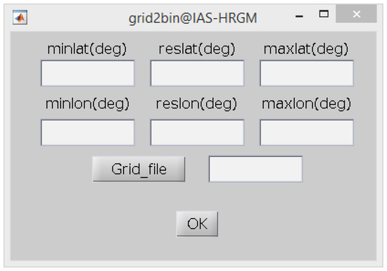
Figure 5.
The ‘grid2bin‘ interface.
4. Validation and Numerical Results
In this section, the TGF software is applied for computation of gravity values implied by the Earth’s global topography (Section 4.1) and for residual (high frequency) gravity effects, as generated by a residual terrain model (RTM, Section 4.2). Both types of computations are compared against independent reference values which have been demonstrated of sub-mGal level accuracy, allowing us to verify the TGF computational results. Further, some optimization experiments are presented showing how the efficiency of the numerical integration can be increased.
4.1. External Validation of the Topographic Field Calculation
In order to demonstrate TGF’s performance in topographic gravity field calculation, the TGF computations have been compared with independent calculations using the in-house Newtonian integrator by Curtin University, as described in [37]. In the Curtin’s Newtonian integrator (CNI), prism and tesseroid are combined for discretization. The CNI has already been comprehensively tested and widely applied in the calculation of topographic gravitational potential up to second-order derivatives [37], the study of spectral characters of band-limited topography generated gravity field [8,38], and the calculation of SRTM2gravity [1,34], showing its capability to provide topographic gravity at a precision level at 0.1 mGal level or better. In this experiment, the gravity field calculated by CNI provides a reference to validate the TGF software. The agreement between gravity field computations from TGF and CNI would provide an insight into the accuracy of the topographic gravity field calculated by TGF software.
For this external validation experiment, the test area was located at the most rugged Himalaya area bounded by 27°N~28°N in latitude and 87°E~88°E in longitude. Topographic heights taken from Multi-Error-Removed Improved-Terrain (MERIT) DEM represent the upper boundary and the EGM96 geoid the lower boundary of the topographic masses. The masses over the entire globe were considered and were subdivided into five zones, approximated and represented by prism to 15° around the computation point and tesseroids to cover the whole globe, up to 180° radius. Table 2 gives the definition of each zone, regularization model, DEM resolution and zones extension used in TGF and CNI. As gravity functional, we calculated two sets of gravity disturbances (radial derivatives of the gravitational potential) at 15″ grid resolution over our study area with CNI ( see previous results by [8] and with TGF () respectively. The topographic gravity disturbances calculated with TGF were then compared to the corresponding values from CNI .
Table 2.
The resolutions and extensions in topographic and RTM gravity field calculation.
Figure 6 and Table 3 show the results of this comparison. The agreement between both calculations is always better than 0.3 mGal, with a mean value of ~ −0.06 mGal and RMS of the differences of 0.07 mGal. Overall, the results of this validation experiment provide a satisfactory check on the TGF software. The statistical results suggest the promising results of TGF software in the full-scale topographic gravity field calculations, and demonstrate its calculation accuracy would to be at ~0.1 mGal level.
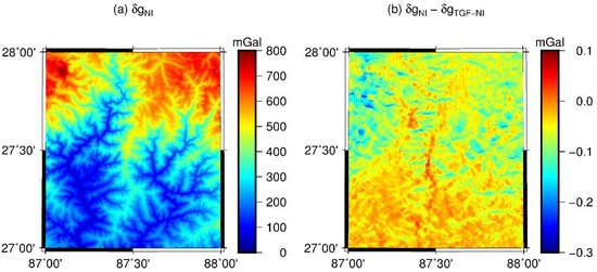
Figure 6.
External validation over Himalaya mountainous area. (a) topographic gravity disturbances calculated by Curtin software , (b) the difference between topographic gravity disturbances calculated by Curtin software and topographic gravity disturbances calculated by TGF software .
Table 3.
External validation for topographic gravity calculation over Himalayas regions (Unit: mGal).
4.2. External Validation of the Residual Gravity Field Calculation
The short-scale (RTM) gravity field modelling capability of TGF is validated here through comparison with a new, highly accurate RTM baseline solution defined in [34]. This RTM baseline solution was obtained from a combination of gravity values from a full-scale global numerical integration (NI) and the long-wavelength signal from spectral-domain gravity forward modelling (SGM). In the full-scale NI method, the topographic masses between the geoid height and the Earth’s surface represented by 3” MERIT DEM were considered. The full-scale gravity signals were evaluated in the spatial domain using CNI with resolution levels and grid extensions displayed in Table 2. The ultra-high degree SGM solution generated by [34] yields the gravity signals implied by the reference topography of MERIT Spherical Harmonic coefficients (SHCs) to degree and order 2160 and provides the long-wavelength signals. In both calculations, a constant density assumption of 2670 kg/m3 was adopted.
The key inputs for RTM gravity field calculations with TGF were upper boundary of 3” MERIT DEM, reference surface of MERIT SHCs to degree 2160, and a constant density value of 2670 kg/m3. For the parameters used in the TGF software, see again Table 2. The residual masses within 1° distance from the calculation point were considered and divided into four zones. Polyhedron and prism with 3” DEM were primarily applied in the vicinity zones and extends up to 0.02° and 0.03° distance around each calculation point, while tesseroid with 3” DEM extending to 0.15°, and point-mass for the outside distances with DEM of 30” resolution. Accordingly, the RTM models high-frequency field signals at spatial scales of ~10 km to ~100 m. The differences between NI and SGM provide the RTM reference solution (cf. [34]) that is used here as an independent check on the RTM gravity calculation with our TGF software.
Validation experiments were carried out over two study areas with extremely rugged topography on the earth-surface: Himalaya mountainous area ( in latitude, and in longitude), and Switzerland around Alpine region ( in latitude, and in longitude). RTM gravity field at 15″ grid on the Earth’s surface was calculated by TGF software and compared with the RTM baseline values. The results and differences are shown in Figure 7 (over Himalayas) and Figure 8 (over Switzerland), descriptive statistics are reported in Table 4. The RMS differences between TGF-based RTM gravity disturbances and reference values from global numerical integration and SGM are smaller than the mGal-level over the two study areas (see Table 4).
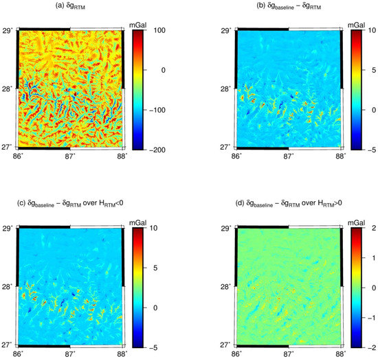
Figure 7.
External validation based on RTM baseline [34] over Himalaya mountainous area. indicates TGF calculated RTM gravity disturbances. (a) TGF calculated RTM gravity disturbance; (b) the difference between RTM calculated gravity disturbance and RTM baseline solution; (c) the differences over points with negative RTM height; (d) the differences over points with positive RTM height. represents RTM height, it is the height difference between surface topography and reference topography, with .
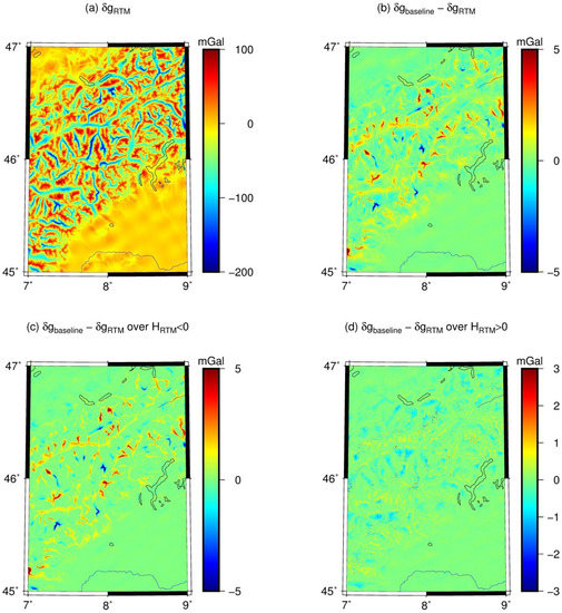
Figure 8.
External validation based on RTM baseline [34] over Switzerland. (a) TGF calculated RTM gravity disturbance; (b) the difference between RTM calculated gravity disturbance and RTM baseline solution; (c) the differences over points with negative RTM height; (d) the differences over points with positive RTM height. indicates TGF calculated RTM gravity disturbances. represents RTM height, it is the height difference between surface topography and reference topography, with .
Table 4.
External validation For RTM gravity calculation over Himalayas and Switzerland Alpine regions (Unit: mGal).
Specifically, for points outside the RTM reference topography (that is, no harmonic correction (HC) was applied), the differences are as low as 0.22 mGal RMS over Himalaya and 0.38 mGal RMS over Switzerland. On the other hand, for points inside the RTM reference topography (that is, the [6] HC was applied in TGF), the approximate character of the HC comes into play. This is seen from increasing RMS errors to the mGal-level (cf. [34]). Overall, our validation results show the sub-mGal computational precision that can be achieved with TGF for residual gravity field computations. Strategies to reduce HC-related approximation errors have been discussed, e.g., in [34], and are not within the scope of the present study.
4.3. Internal Validation and Numerical Efficiency
An important aspect of topographic gravitational field calculations is the computational effort related to the evaluation of Newtonian integration. The calculation time is linearly correlated with the number of calculation points and the resolution of integration masses. Many procedures for an efficient calculation of the topography implied gravitational field have been proposed. For instance, one approach is to split the topographic masses into two parts according to wavelengths [1,34]: the long-wavelength signal could be efficiently achieved through SGM, while the residual short-wavelength parts are modeled in the spatial domain through RTM technique with numerical integration radius being restricted to the neighbourhood of evaluation points. In the following studies, RTM masses is modeled as the residual masses between the earth surface (represented by 3″ MERIT DEM by [39]) and reference surface (SHCs to degree 2,160 directly derived from 3” MERIT DEM via spherical harmonic analysis [34]).
The spatial-domain numerical evaluation methods have been developed and programmed for given geometries (polyhedron, prism, tesseroid and point-mass) in the TGF software. However, as discussed above, the computation time often appears as a limiting practical issue considering specific geometry for large or complex problems. Depending on the attenuation and fluctuation nature of RTM gravitational field, the geometry switches relying on the trade-off between accuracy and efficiency, and coarse DEM is adopted and truncated in a distant zone.
The trade-off between achieved RTM accuracy and computation efficiency is investigated through a comparison with a defined internal testbed. In the experiment, the internal testbed was defined by the RTM gravity disturbances calculated from a set of optimal integration parameters, i.e., polyhedron with 3” DEM within the vicinity of 0.33° distance, tesseroid with 3” DEM extending to 1°, and point-mass for outside and truncated to 2°. The values of the internal testbed provide reference values for the internal validation tests.
In the internal validation, 576 calculation points are homogeneously distributed (at 15″ grid resolution) on the surface of the Earth’s roughest Himalaya area within the , where forward modelling errors can be expected to be largest. The RTM gravity disturbances over 576 points are calculated with various combinations of geometry and radius, then compared with internal testbed. In order to investigate the forward modeling accuracy and computation time with radius choices of polyhedron and prism, the following procedure for international validation was followed:
(1) Internal testbed calculation over 576 points, with ;
(2) The radius dataset definition, where , , with fixed ;
(3) Implementing forward modelling procedure to get RTM gravity field data set with radius combination, and record calculation efficiency;
(4) Residuals’ evaluation through comparison between data set with internal testbed . They indicate the error level that can be attributed to the variation of regularization with polyhedron and prism.
(5) Statistical analysis of RMS values of each set of residuals.
The internal validation results are shown in Figure 9. Figure 9a displays the RMS values of residual gravity disturbances. With increasing of polyhedron radius from to , the results show a boost in accuracy, from several mGal to less 1mGal. To achieve 1 mGal accuracy, polyhedron should be extended farther than distance from calculation point. Because of the gravity attenuation character, using polyhedron far than would gain little improvement. From Figure 9b, it is obvious that accurate computation always compromises to efficiency. Using polyhedron extending to , the software could achieve the calculation efficiency of 10 points per second.
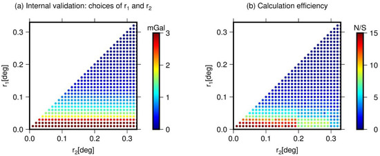
Figure 9.
Forward modelling evaluation accuracy and efficiency with various radius choices of polyhedron and prism. (a) RMS in mGal of internal comparison. (b) calculation efficiency in N/S (number per second). extension radius of polyhedron and radius of prism.
A further experiment investigates the choices of tesseroid and point-mass. The extensions are implemented with , , and fixed . The computed RTM gravity disturbances, based on each radius dataset, are then compared with the internal testbed. The results are shown in Figure 10. It demonstrates that with increasing radius, computation generally takes more time, from 10 points per second to more than 10 seconds per point. The RMS of discrepancies less than 1 mGal when tesseroid radius is extended to 0.1° and point-mass up to distance of 0.5°. More safely, are recommended for 1 mGal accurate RTM gravity signal retrieving using TGF software. However, for most of areas where topography is smoother than that of test area (Himalaya area), the results based on are accurate enough to recover 1 mGal gravity signals implied by the topography.
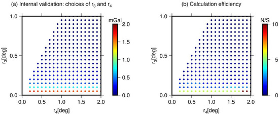
Figure 10.
Forward modelling evaluation accuracy and efficiency with various radius choices of tesseroid and point mass. (a) RMS in mGal of internal comparison. (b) calculation efficiency in N/S (number of points per second). extension radius of tesseroid and radius of point mass.
4.4. RTM Gravity Field over Zugspitze Area
In order to exemplify the spectrum of the implemented gravity field functionals, from potential values to first- and second-order derivatives, the TGF software was applied for regional RTM gravity field calculations over a test area located in the Zugspitze of German Alps (with longitude between 10.95 and 11.25, and latitude between 47.35 and 47.5). With MERIT DEM and MERIT SHCs 2160 respectively representing the Earth’s surface and the smooth reference surface, the residual (RTM) heights vary from -600 m to 1200 m (Figure 11). This makes the test area a good example for high-frequency gravity field studies over mountain areas.
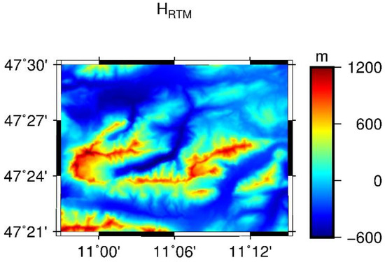
Figure 11.
Residual height over Zugspitze (German Alps) area.
The gravity field functionals, calculated for 972,000 points, arranged in terms of a 1″ resolution grid, are displayed in Figure 12 and Figure 13. All computations use a constant density of 2670 kg/m3 and spherical approximation, and the regularization and discretization method follows the parameters listed in Table 2. In order to avoid numerical instabilities for the tensor components, the calculation points are located 1 m above the Earth’s surface rather than on the Earth’s surface itself.
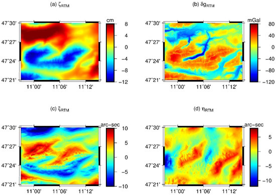
Figure 12.
Residual gravity field calculated by TGF software, indicates residual geoid height signals, residual gravity disturbances, and represent north-south and east-west components of vertical deflection separately.
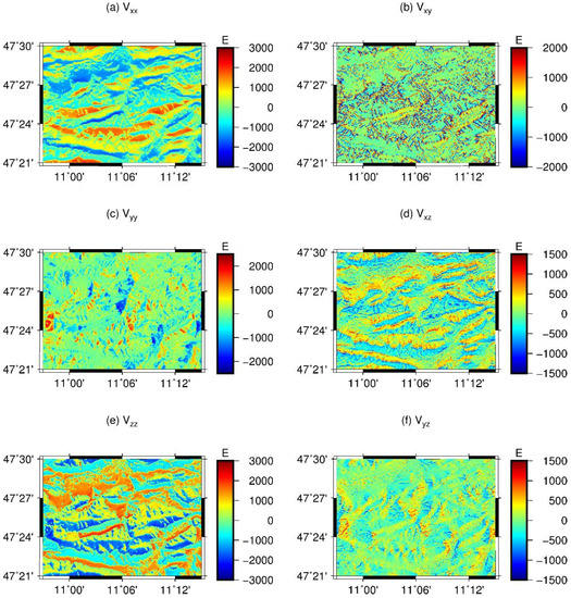
Figure 13.
Marussi Tensor components over Zugspitze (German Alps) area.
Figure 12 displays the calculated: panel (a)—residual geoid heights (varying from ~ 12 cm to ~ 8 cm, Panel (b)—residual gravity disturbance ranging from ~ −120 mGal to ~ 80 mGal, and north-south (Panel (c)) and east-west (Panel (d)) components of vertical deflections. The large magnitude of these components shows the relevance of high-frequency gravity signals in global or regional gravity field determination.
Figure 13 shows the calculated elements of the Marussi tensor, with the first column illustrating the diagonal components (Panel (a)), (Panel (c)) and (Panel (e)), and the second column the off-diagonal components (Panel (b)), (Panel (d)) and (Panel (f)). TGF may prove to be a beneficial tool for studying the short-scale signal characteristics of the high-order derivatives of the potential together with highly detailed elevation models.
5. Conclusions and Applications
The fast and accurate calculation of gravity field functionals generated by a mass-density distribution of arbitrary-shaped 3D geometries is a prerequisite for many geodetic and geophysical applications. In this contribution, we developed the new MATLAB-tool TGF to compute the gravity field implied by terrain masses in the spatial domain. The source code and user manual related to the TGF software are provided in the Supplementary Materials. Compared to the most up-to-date MATLAB tool GTeC, our TGF software (1) includes more efficient geometries, i.e., tesseroid and point-mass, (2) enables calculation of full-scale and high-frequency gravity field functionals including (3) the gravitational potential, its gradients and second derivatives, (4) considers the curvature of the Earth by involving spherical approximation and ellipsoidal approximation.
The external validations have been carried out via the comparisons with reference values. In the first experiments, two sets of full-scale topographic gravity disturbances were calculated using the Newtonian integrator of Curtin University and using the TGF software, respectively. These calculations were based on the same DEM inputs, density assumption, and similar discretization methods. The differences between calculated gravity disturbances indicate the uncertainties in scientific software and computation. In the second experiment, comparisons were drawn between a RTM baseline solution through a combination of SGM and NI method and RTM results calculated by the TGF software. With same inputs for both calculations, the comparison results show the error level that can be attributed to methodologies applied in the TGF software and the baseline solution. Both validation experiments were conducted over the roughest Himalaya area, where large forward modelling errors can be expected. The comparisons indicate the sub-mGal level accuracy of the TGF in the calculation of the full-scale topographic and RTM gravity field. Over valleys, large errors up to around 10 mGal are encountered which were attributed to the applied condensation harmonic correction technique.
Precise gravity forward modelling generally requires the use of complex geometrical bodies such as polyhedra but at the expense of efficiency in the numerical evaluation. In this study, the trade-off between accuracy and efficiency was investigated based on the internal validation. In this experiment, 576 calculation points are located on the surface of the Earth’s roughest Himalaya area. Gravity disturbances were calculated with various values of integration radii for each zone and compared with an internal testbed solution using a set of optimum integration parameters. Based on the trade-off study between accuracy and efficiency, a set of parameters () are recommended for RTM gravity field calculations of accuracy at 1 mGal level and efficiency of around 10 points per second when using 3″ DEM in the vicinity of the computation point. This demonstrates the TGF’s potential for processing high-resolution DEMs associated with roughest topography. However, the integration radii for each zone are also affected by the roughness of the local topography, resolution of applied DEMs and variations of geological density.
The new TGF software has been found to be well suited for demanding scientific tasks related to the numerical evaluation of Newton’s integral. For example, the TGF software has already been extensively tested and recently been applied in the SRTM2gravity project [1] to successfully convert the global 3” SRTM topography to implied gravity effects at about 28 billion computation points. In this project, the TGF software was applied in high-frequency (finer than 10 km) residual gravity signal calculation, and then combined with the long- and medium-wavelength gravity signal from spectral gravity forward modelling at an accuracy level better than 1 mGal. In [33], the TGF software was tested by comparison with precomputed gravity effects from the ERTM2160 gravity model, and TGF was also utilized to study the use of mass-density maps in gravity forward modelling. In New Zealand, a mass-density map together with RTM technique were combined to investigate the lateral density variation effect in high-frequency gravity signal calculation. Besides, depending on the input elevation grids, which define the boundaries of forward masses, the TGF is capable of calculating various gravity field functionals, implied by the topography gravity field or high-frequency gravity field. TGF was used in [40] to study the tree bias effect on gravity forward modelling. The topographic and RTM gravity disturbances were calculated based on SRTM DEM (containing tree bias) and MERIT DEM (representing the bare-ground surface) separately. The differences between SRTM-based forward modelling results and MERIT-based results indicated the tree bias effect in gravity forward modelling. It is our hope that the TGF software proves beneficial to the geodetic and geophysical user community.
Supplementary Materials
The Terrain Gravity Field (TGF) software is freely available online at https://www.lrg.tum.de/iapg/forschung/schwerefeld/tgf/.
Author Contributions
C.H. developed the idea to create the forward modelling software and defined the required software capabilities. M.Y. was responsible for the software implementation and carried out all numerical tests and validation experiments, created all figures and tables in the paper, and wrote the first draft of the manuscript. All authors discussed and commented on the manuscript. All authors have read and agreed to the published version of the manuscript
Acknowledgments
We would like to thank the Chinese Scholarship Council for providing funding under scholarship no 201504910729.
Conflicts of Interest
The authors declare no conflict of interest.
References
- Hirt, C.; Yang, M.; Kuhn, M.; Bucha, B.; Kurzmann, A.; Pail, R. SRTM2gravity: An Ultrahigh Resolution Global Model of Gravimetric Terrain Corrections. Geophys. Res. Lett. 2019, 46, 4618–4627. [Google Scholar] [CrossRef]
- Forsberg, R.; Tscherning, C.C. The use of height data in gravity field approximation by collocation. J. Geophys. Res. Solid Earth 1981, 86, 7843–7854. [Google Scholar] [CrossRef]
- Tziavos, I.N.; Sideris, M.G. Topographic Reductions in Gravity and Geoid Modeling. In Geoid Determination; Sansò, F., Sideris, M.G., Eds.; Springer: Berlin/Heidelberg, Germany, 2013. [Google Scholar] [CrossRef]
- Elhabiby, M.; Sampietro, D.; Sansò, F.; Sideris, M.G. BVP, Global Models and Residual Terrain Correction. In Observing our Changing Earth; Springer: Berlin/Heidelberg, Germany, 2009; pp. 211–217. [Google Scholar] [CrossRef]
- Makhloof, A.A.; Ilk, K.H. Effects of topographic–isostatic masses on gravitational functionals at the Earth’s surface and at airborne and satellite altitudes. J. Geod. 2007, 82, 93–111. [Google Scholar] [CrossRef]
- Forsberg, R. A Study of Terrain Reductions, Density Anomalies and Geophysical Inversion Methods in Gravity Field Modelling; The Ohio State University: Columbus, OH, USA, 1984. [Google Scholar]
- Hirt, C. RTM Gravity Forward-Modeling Using Topography/Bathymetry Data to Improve High-Degree Global Geopotential Models in the Coastal Zone. Mar. Geod. 2013, 36, 183–202. [Google Scholar] [CrossRef]
- Hirt, C.; Reußner, E.; Rexer, M.; Kuhn, M. Topographic gravity modeling for global Bouguer maps to degree 2160: Validation of spectral and spatial domain forward modeling techniques at the 10 microGal level. J. Geophys. Res. Solid Earth 2016, 121, 6846–6862. [Google Scholar] [CrossRef]
- Sánchez, L.; Sideris, M.G. Vertical datum unification for the International Height Reference System (IHRS). Geophys. J. Int. 2017, 209, 570–586. [Google Scholar] [CrossRef]
- Balmino, G.; Vales, N.; Bonvalot, S.; Briais, A. Spherical harmonic modelling to ultra-high degree of Bouguer and isostatic anomalies. J. Geod. 2011, 86, 499–520. [Google Scholar] [CrossRef]
- Hirt, C.; Kuhn, K. Evaluation of high-degree series expansions of the topographic potential to higher-order powers. J. Geophys. Res. Solid Earth 2012, 117. [Google Scholar] [CrossRef]
- Rexer, M. Spectral Solutions to the Topographic Potential in the context of High-Resolution Global Gravity Field Modelling. Doctoral Dissertation, Technical University of Munich, Munich, Germany, 2017. [Google Scholar]
- Bucha, B.; Hirt, C.; Kuhn, M. Cap integration in spectral gravity forward modelling: Near- and far-zone gravity effects via Molodensky’s truncation coefficients. J. Geod. 2008, 93, 65–83. [Google Scholar] [CrossRef]
- Wieczorek, M.A.; Meschede, M. SHTools: Tools for Working with Spherical Harmonics. Geochem. Geophys. Geosyst. 2018, 19, 2574–2592. [Google Scholar] [CrossRef]
- Rexer, M.; Hirt, C. 2015 Ultra-high-Degree SHA Gauss–Legendre Driscoll/Healy Quadrature Theorem Earth, Mars and Moon. Surv. Geophys. 2015, 36, 803–830. [Google Scholar] [CrossRef]
- Rexer, M.; Hirt, C.; Claessens, S.; Tenzer, R. Layer-Based Modelling of the Earth’s Gravitational Potential up to 10-km Scale in Spherical Harmonics in Spherical and Ellipsoidal Approximation. Surv. Geophys. 2016, 37, 1035–1074. [Google Scholar] [CrossRef]
- Grombein, T.; Seitz, K.; Heck, B. The Rock–Water–Ice Topographic Gravity Field Model RWI_TOPO_2015 and Its Comparison to a Conventional Rock-Equivalent Version. Surv. Geophys. 2016, 37, 937–976. [Google Scholar] [CrossRef]
- Rexer, M.; Hirt, C.; Pail, R. High-resolution global forward modelling - A degree-5480 global ellipsoidal topographic potential model. Eur. Geosci. Union Gen. Assembl. 2017, 19, 7725. [Google Scholar]
- Abrykosov, O.; Ince, E.S.; Foerste, C.; Flechtner, F. Rock-Ocean-Lake-Ice Topographic Gravity Field model (ROLI Model) Expanded up to Degree 3660. Available online: http://doi.org/10.5880/ICGEM.2019.011 (accessed on 13 January 2020).
- Tsoulis, D.; Novák, P.; Kadlec, M. Evaluation of precise terrain effects using high-resolution digital elevation models. J. Geophys. Res. 2009, 114, B02404. [Google Scholar] [CrossRef]
- Hwang, C.; Wang, C.G.; Hsiao, Y.S. Terrain correction computation using Gaussian quadrature. Comput. Geosci. 2003, 29, 1259–1268. [Google Scholar] [CrossRef]
- Uieda, L.; Barbosa, V.C.F.; Braitenberg, C. Tesseroids: Forward-modeling gravitational fields in spherical coordinates. Geophysics 2016, 81, F41–F48. [Google Scholar] [CrossRef]
- Tsoulis, D. Analytical computation of the full gravity tensor of a homogeneous arbitrarily shaped polyhedral source using line integrals. Geophysics 2012, 77, F1–F11. [Google Scholar] [CrossRef]
- Wild-Pfeiffer, F. A comparison of different mass elements for use in gravity gradiometry. J. Geod. 2008, 82, 637–653. [Google Scholar] [CrossRef]
- Cella, F. GTeC—A versatile MATLAB® tool for a detailed computation of the terrain correction and Bouguer gravity anomalies. Comput. Geosci. 2015, 84, 72–85. [Google Scholar] [CrossRef]
- Hirt, C.; Claessens, S.; Fecher, T.; Kuhn, M.; Pail, R.; Rexer, M. New ultrahigh-resolution picture of Earth’s gravity field. Geophys. Res. Lett. 2013, 40, 4279–4283. [Google Scholar] [CrossRef]
- Haeger, C.; Kaban, M.K.; Tesauro, M.; Petrunin, A.G.; Mooney, W.D. 3-D Density, Thermal, and Compositional Model of the Antarctic Lithosphere and Implications for Its Evolution. Geochem. Geophys. Geosyst. 2019, 20, 688–707. [Google Scholar] [CrossRef]
- Abd-Elmotaal, H.A. Gravimetric geoid for Egypt implementing Moho depths and optimal geoid fitting approach. Stud. Geophys. Geod. 2017, 61, 657–674. [Google Scholar] [CrossRef]
- Nagy, D.; Papp, G.; Benedek, J. The gravitational potential and its derivatives for the prism. J. Geod. 2000, 74, 552–560. [Google Scholar] [CrossRef]
- Nagy, D.; Papp, G.; Benedek, J. Corrections to “The gravitational potential and its derivatives for the prism”. J. Geod. 2002, 76, 475. [Google Scholar] [CrossRef]
- Heck, B.; Seitz, K. A comparison of the tesseroid, prism and point-mass approaches for mass reductions in gravity field modelling. J. Geod. 2006, 81, 121–136. [Google Scholar] [CrossRef]
- Grombein, T.; Seitz, K.; Heck, B. Optimized formulas for the gravitational field of a tesseroid. J. Geod. 2013, 87, 645–660. [Google Scholar] [CrossRef]
- Yang, M.; Hirt, C.; Tenzer, R.; Pail, R. Experiences with the use of mass-density maps in residual gravity forward modelling. Stud. Geophys. Geod. 2018, 62, 596–623. [Google Scholar] [CrossRef]
- Hirt, C.; Bucha, B.; Yang, M.; Kuhn, M. A numerical study of residual terrain modelling (RTM) techniques and the harmonic correction using ultra-high-degree spectral gravity modelling. J. Geod. 2019, 93, 1469–1486. [Google Scholar] [CrossRef]
- Laske, G.; Masters, G.; Ma, Z.T.; Pasyanos, M. Update on CRUST1.0 A 1-degree Global Model of Earth’s Crust. In Proceedings of the EGU General Assembly, Vienna, Austria, 23–28 April 2013. [Google Scholar]
- Tenzer, R.; Sirguey, P.; Rattenbury, M.; Nicolson, J. A digital rock density map of New Zealand. Comput. Geosci. 2011, 37, 1181–1191. [Google Scholar] [CrossRef]
- Kuhn, M.; Hirt, C. Topographic gravitational potential up to second-order derivatives: An examination of approximation errors caused by rock-equivalent topography (RET). J. Geod. 2016, 90, 883–902. [Google Scholar] [CrossRef]
- Hirt, C.; Kuhn, M. Band-limited topographic mass distribution generates full-spectrum gravity field: Gravity forward modeling in the spectral and spatial domains revisited. J. Geophys. Res. Solid Earth 2014, 119, 3646–3661. [Google Scholar] [CrossRef]
- Yamazaki, D.; Ikeshima, D.; O’Loughlin, F.e.a. A high-accuracy map of global terrain elevations. Geophys. Res. Lett. 2017, 44, 5844–5853. [Google Scholar] [CrossRef]
- Yang, M.; Hirt, C.; Rexer, M.; Pail, R.; Yamazaki, D. The tree-canopy effect in gravity forward modelling. Geophys. J. Int. 2019, 219, 271–289. [Google Scholar] [CrossRef]
© 2020 by the authors. Licensee MDPI, Basel, Switzerland. This article is an open access article distributed under the terms and conditions of the Creative Commons Attribution (CC BY) license (http://creativecommons.org/licenses/by/4.0/).