Discharge Estimates for Ungauged Rivers Flowing over Complex High-Mountainous Regions based Solely on Remote Sensing-Derived Datasets

 , , ,
, , , 
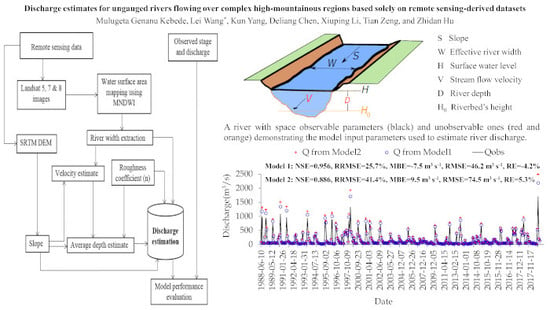
Abstract
1. Introduction
2. Materials and Methods
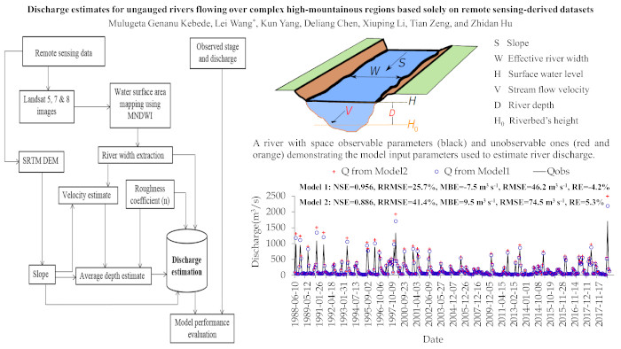
2.1. Study Area
2.2. Data
2.3. Methodology
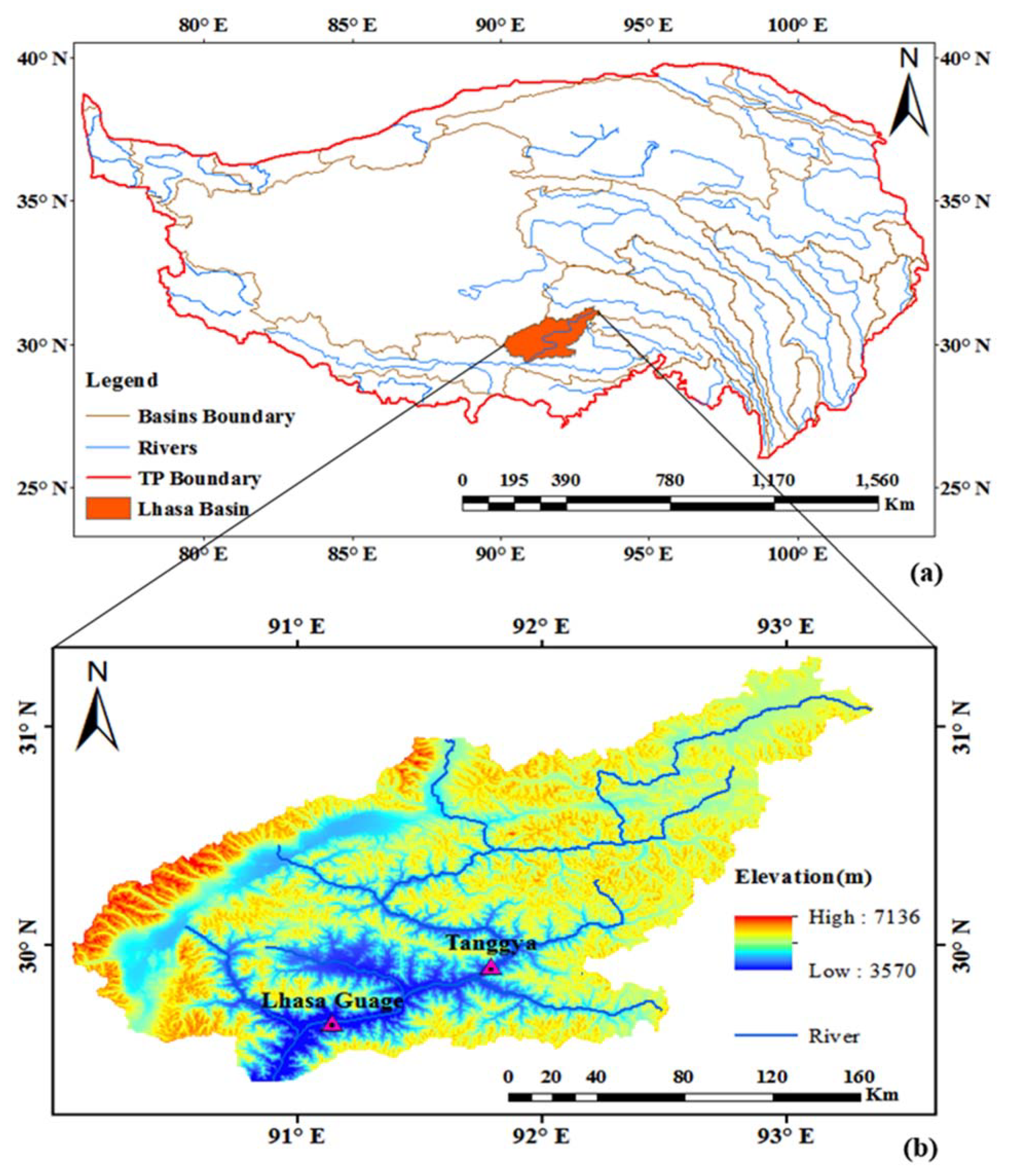
2.3.1. Estimating Water Surface Area (WSA) and Effective Width (W)
2.3.2. Estimating Channel Slope (S)
2.3.3. Estimating Channel Roughness Coefficient (n)
2.3.4. Estimating River Depth and Velocity
2.3.5. Estimating River Discharge
2.3.6. Evaluation of Models Performance
3. Results
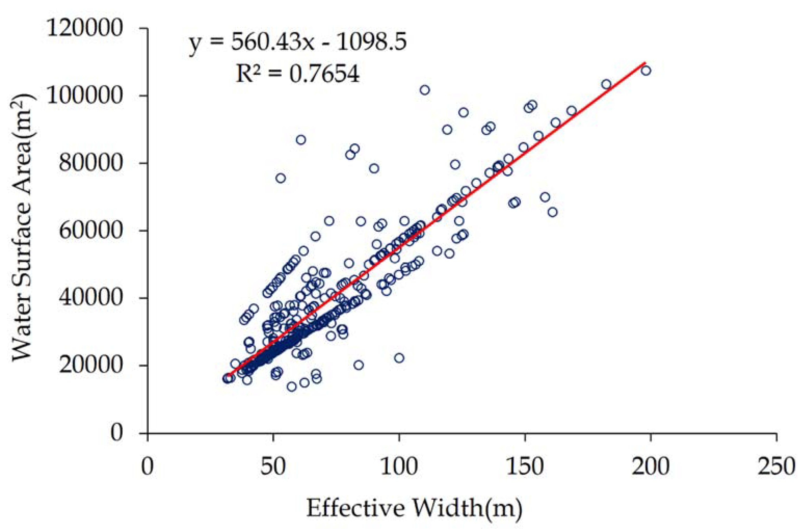
3.1. Water Surface Area (WSA) and Width
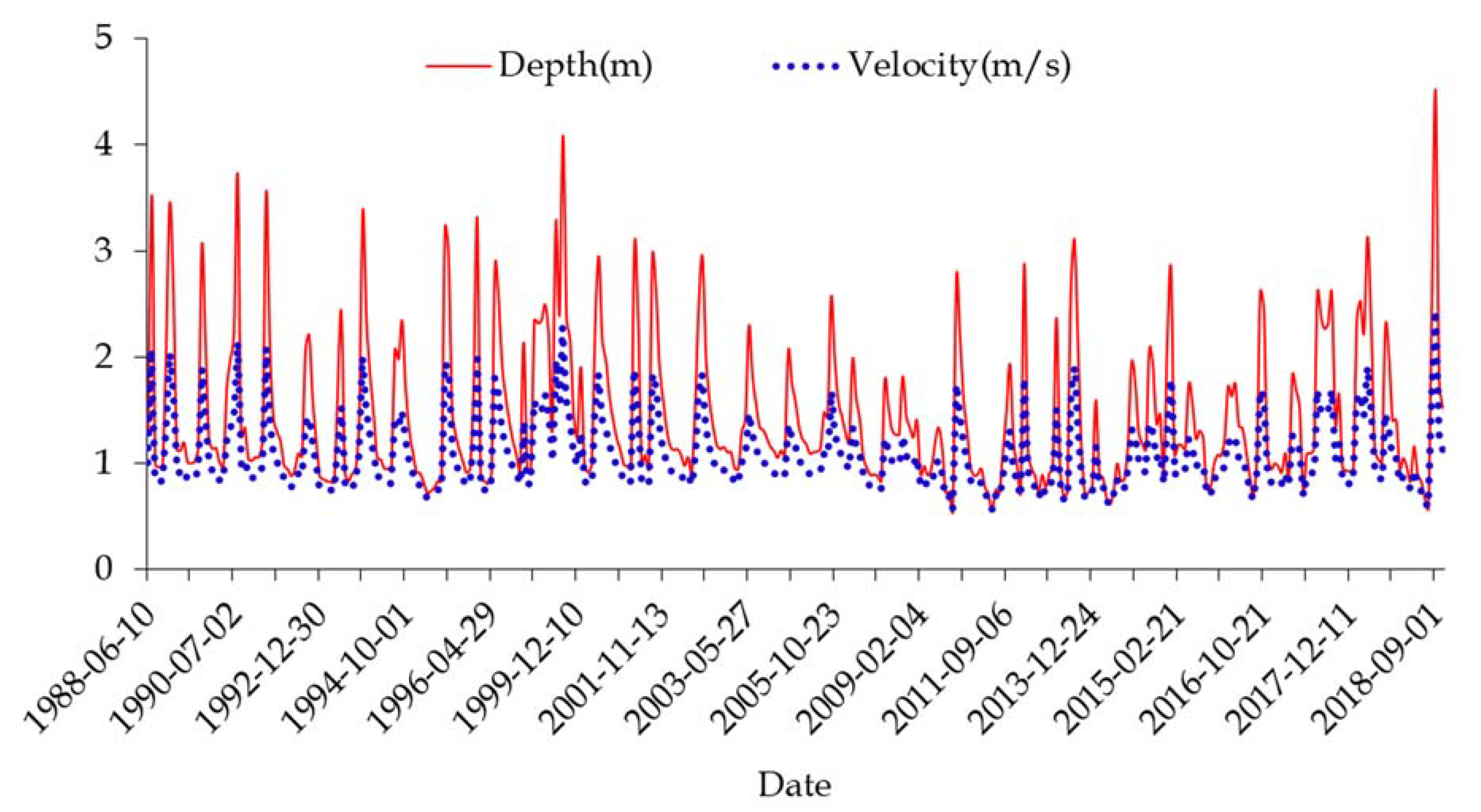
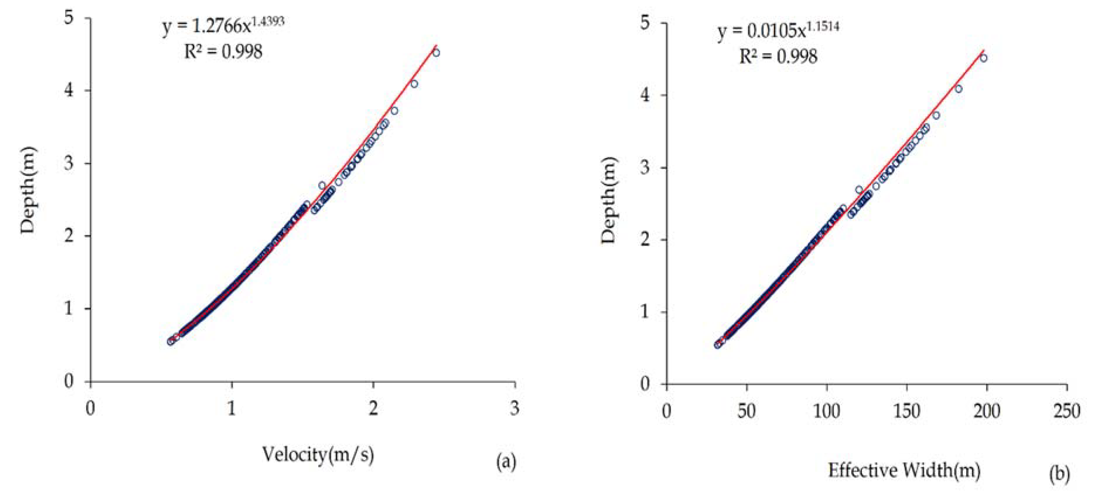
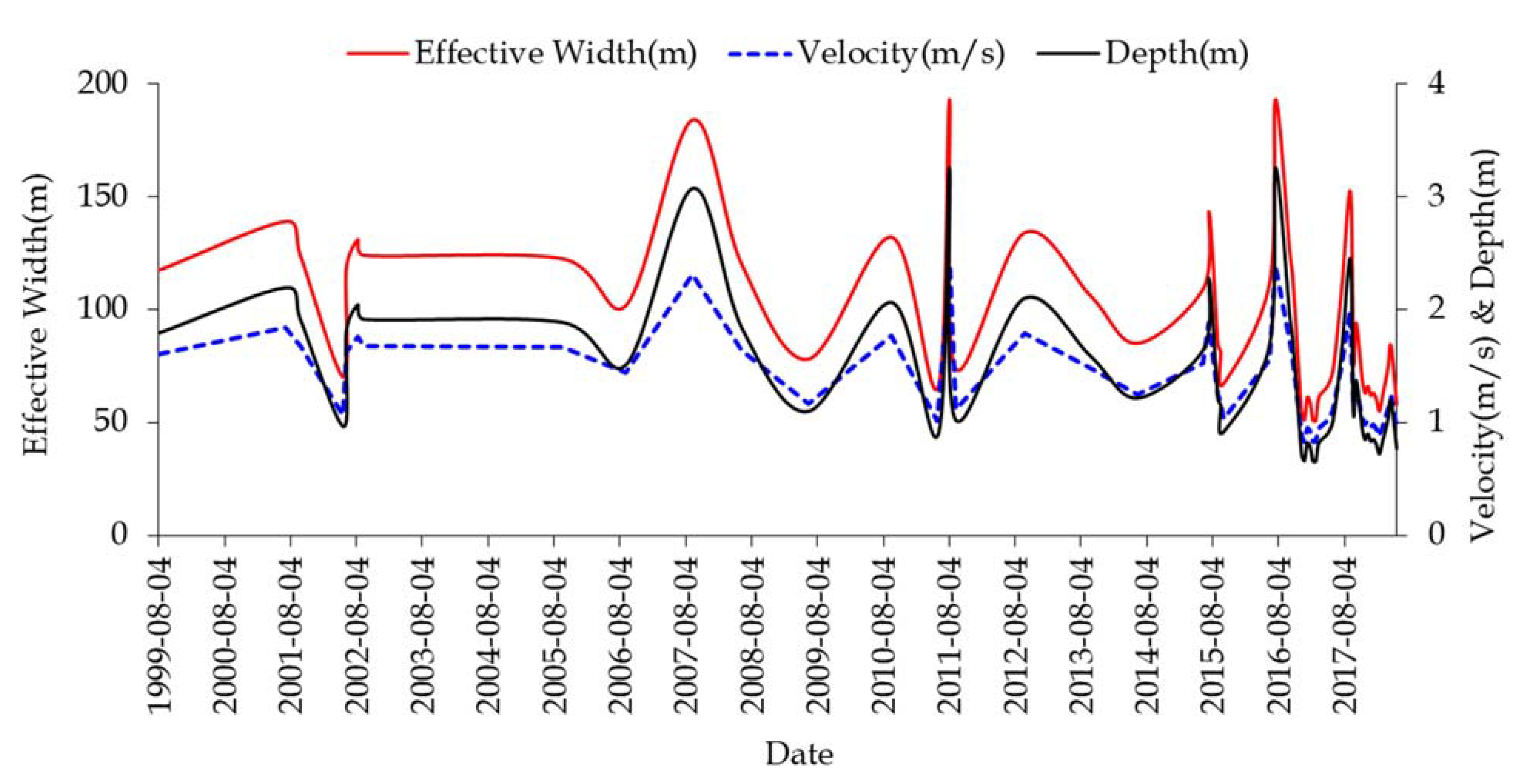
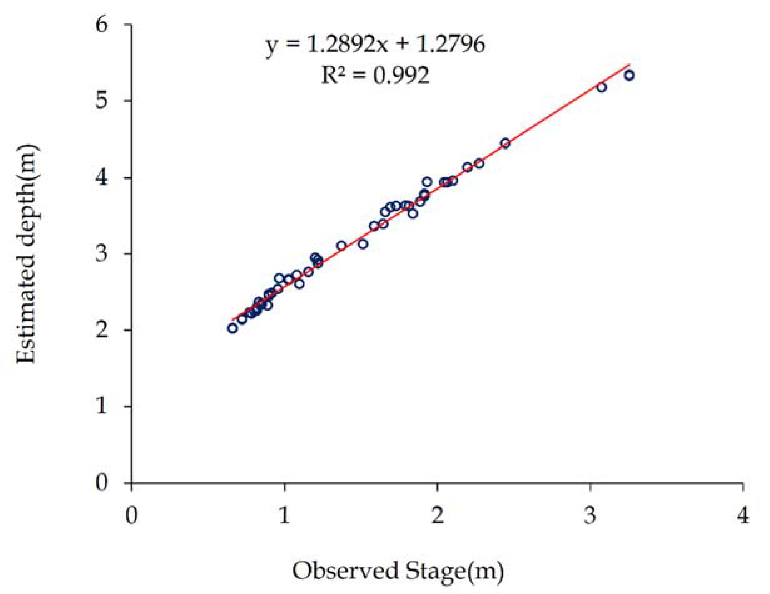
3.2. River Depth and Velocity
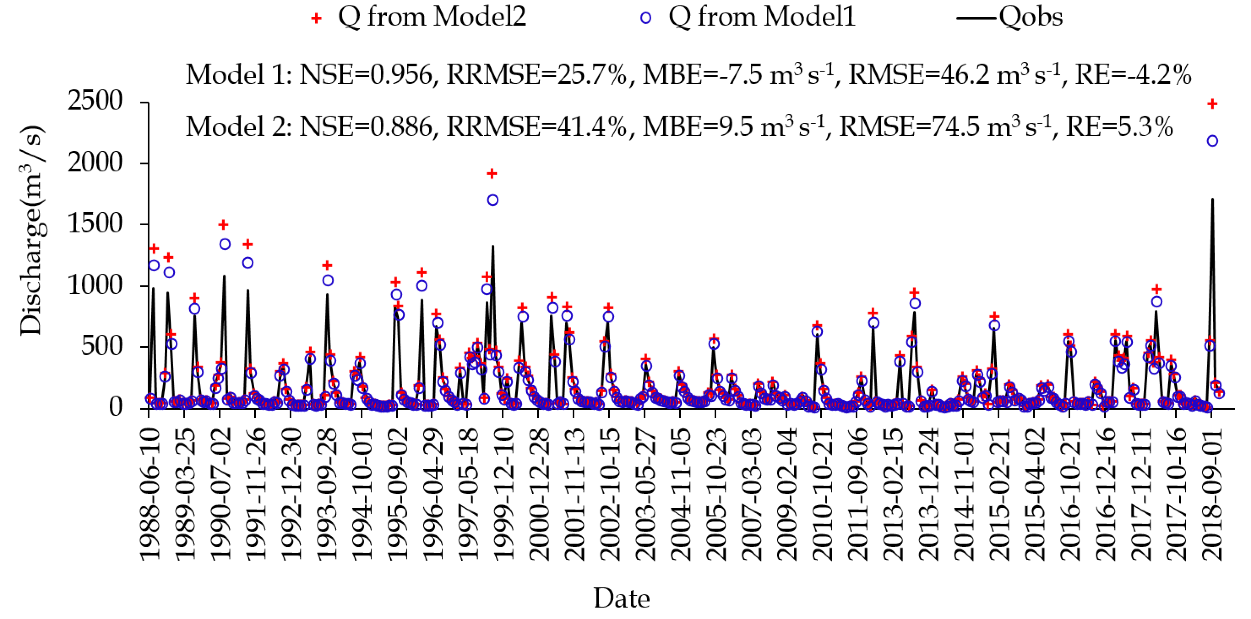
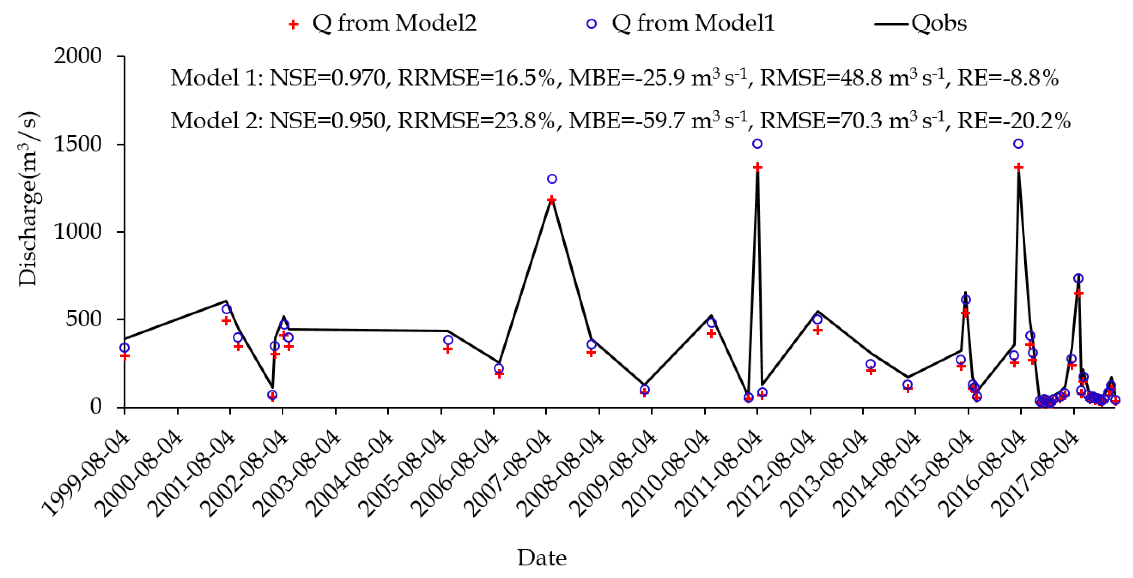
3.3. River Discharge
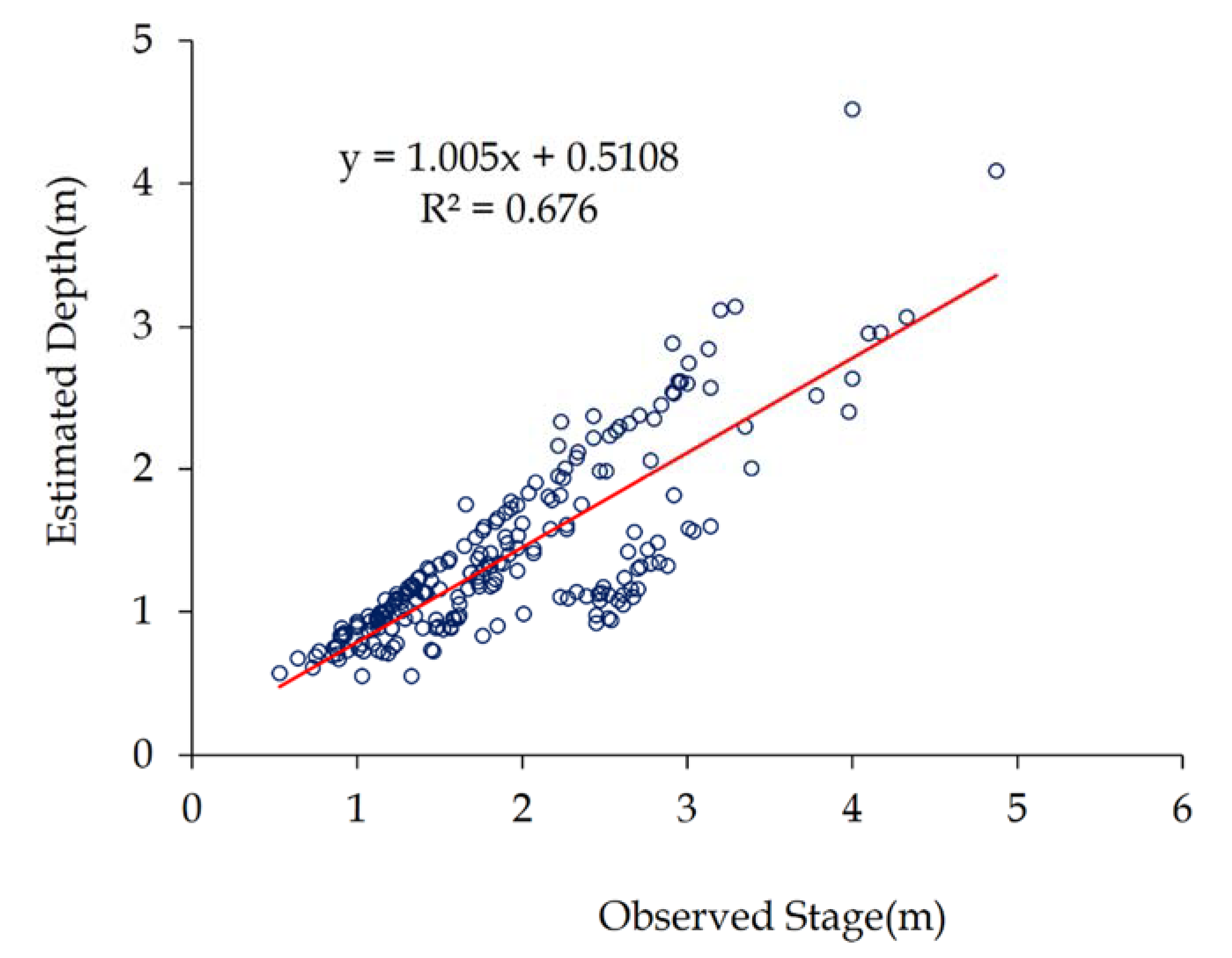
3.4. Further Validation of the Methodology
4. Discussions
5. Conclusions
Author Contributions
Acknowledgments
Data Availability Statement
Conflicts of Interest
References
- Durand, M.; Gleason, C.J.; Garambois, P.A.; Bjerklie, D.; Smith, L.C.; Roux, H.; Rodriguez, E.; Bates, P.D.; Pavelsky, T.M.; Monnier, J.; et al. An intercomparison of remote sensing river discharge estimation algorithms from measurements of river height, width, and slope. Water Resour. Res. 2016, 52, 4527–4549. [Google Scholar] [CrossRef]
- Oki, T.; Kanae, S. Global hydrological cycles and world water resources. Science 2006, 313, 1068–1072. [Google Scholar] [CrossRef] [PubMed]
- Dai, A.; Trenberth, K.E. Estimates of freshwater discharge from continents: Latitudinal and seasonal variations. J. Hydrometeorol. 2002, 3, 660–687. [Google Scholar] [CrossRef]
- Pavelsky, T.M.; Durand, M.T.; Andreadis, K.M.; Beighley, R.E. Assessing the potential global extent of SWOT river discharge observation. J. Hydrol. 2014, 519, 1516–1525. [Google Scholar] [CrossRef]
- Elmi, O.; Tourian, M.J.; Sneeuw, N. Dynamic River masks from multi-temporal satellite imagery: An automatic algorithm using graph cuts optimization. Remote Sens. 2016, 8, 1005. [Google Scholar] [CrossRef]
- Mersel, M.K.; Smith, L.C.; Andreadis, K.M.; Durand, M.T. Estimation of river depth from remotely sensed hydraulic relationships. Water Resour. Res. 2013, 49, 3165–3179. [Google Scholar] [CrossRef]
- Alsdorf, D.E.; Rodrı´guez, E.; Lettenmaier, D.P. Measuring surface water from space. Rev. Geophys. 2007, 45, RG2002. [Google Scholar] [CrossRef]
- Xu, M.; Kang, S.; Chen, X.; Wu, H.; Wang, X.; Su, Z. Detection of hydrological variations and their impacts on vegetation from multiple satellite observations in the Three-River Source Region of the Tibetan Plateau. Sci. Total Environ. 2018, 639, 1220–1232. [Google Scholar] [CrossRef]
- Tarpanelli, A.; Barbetta, S.; Brocca, L.; Moramarco, T. River discharge estimation by using altimetry data and simplified flood routing modeling. Remote Sens. 2013, 5, 4145–4162. [Google Scholar] [CrossRef]
- Huang, Q.; Long, D.; Dua, M.; Zeng, C.; Qiao, G.; Li, X.; Hou, A. Discharge estimation in high-mountain regions with improved methods using multisource remote sensing: A case study of the Upper Brahmaputra River. Remote Sens. Environ. 2018, 219, 115–134. [Google Scholar] [CrossRef]
- Sichangi, A.W.; Wang, L.; Yang, K.; Chen, D.; Wang, Z.; Li, X.; Zhou, J. Estimating continental river basin discharges using multiple remote sensing data sets. Remote Sens. Environ. 2016, 179, 36–53. [Google Scholar] [CrossRef]
- Dai, A.; Qian, T.; Trenberth, K.E.; Milliman, J.D. Changes in continental freshwater discharge from 1948 to 2004. J. Clim. 2009, 22, 2773–2792. [Google Scholar] [CrossRef]
- Alsdorf, D.E.; Bates, P.; Melack, J.; Wilson, M.; Dunne, T. Spatial and temporal complexity of the Amazon flood measured from space. Geophys. Res. Lett. 2007, 34, L08402. [Google Scholar] [CrossRef]
- Hossain, F.; Siddique-E.-Akbor, A.; Mazumder, L.; ShahNewaz, S.; Biancamaria, S.; Lee, H.; Shum, C. Proof of concept of an altimeter-based river forecasting system for transboundary flow inside Bangladesh. IEEE J. Sel. Top. Appl. Earth Obs. Remote Sens. 2014, 7, 587–601. [Google Scholar] [CrossRef]
- Bjerklie, D.M.; Dingman, S.L.; Vorosmarty, C.J.; Bolster, C.H.; Congalton, R.G. Evaluating the potential for measuring river discharge from space. J. Hydrol. 2003, 278, 17–38. [Google Scholar] [CrossRef]
- Neal, J.; Schumann, G.; Bates, P.; Buytaert, W.; Matgen, P.; Pappenberger, F. A data assimilation approach to discharge estimation from space. Hydrol. Process. 2009, 23, 3641–3649. [Google Scholar] [CrossRef]
- Zhao, C.S.; Pan, T.L.; Xia, J.; Yang, S.T.; Zhao, J.; Gan, X.J.; Hou, L.P.; Ding, S.Y. Streamflow calculation for medium-to-small Rivers in data scarce inland areas. Sci. Total Environ. 2019, 693, 133571. [Google Scholar] [CrossRef]
- Genanu, M.K.; Wang, L.; Li, X.; Hu, Z. Remote sensing-based river discharge estimation for a small river flowing over the high mountain regions of the Tibetan Plateau. Int. J. Remote Sens. 2020, 41, 3322–3345. [Google Scholar] [CrossRef]
- Smith, L.C. Satellite remote sensing of river inundation area, stage, and discharge: A review. Hydrol. Process. 1997, 11, 1427–1439. [Google Scholar] [CrossRef]
- Durand, M.; Rodriguez, E.; Alsdorf, D.E.; Trigg, M. Estimating river depth from remote sensing swath interferometry measurements of river height, slope, and width. IEEE J. Sel. Top. Appl. Earth Obs. Remote Sens. 2010, 3, 20–31. [Google Scholar] [CrossRef]
- Wang, L.; Sichangi, A.W.; Zeng, T.; Li, X.; Hu, Z.; Genanu, M. New methods designed to estimate the daily discharges of rivers in the Tibetan Plateau. Sci. Bull. 2019, 64, 418–421. [Google Scholar] [CrossRef]
- Yang, S.; Wang, J.; Wang, P.; Gong, T.; Liu, H. Low Altitude Unmanned Aerial Vehicles (UAVs) and Satellite Remote Sensing Are Used to Calculated River Discharge Attenuation Coefficients of Ungauged Catchments in Arid Desert. Water 2019, 11, 2633. [Google Scholar] [CrossRef]
- Koutalakis, P.; Tzoraki, O.; Zaimes, G. UAVs for hydrologic scopes: Application of a low-cost UAV to estimate surface water velocity by using three different image-based methods. Drones 2019, 3, 14. [Google Scholar] [CrossRef]
- Gentile, V.; Mróz, M.; Spitoni, M. Bathymetric mapping of shallow rivers with UAV hyperspectral data. In Proceedings of the 5th International Conference on Telecommunications and Remote Sensing, Milan, Italy, 10 October 2016; pp. 43–48. [Google Scholar] [CrossRef]
- Papa, F.; Durand, F.; Rossow, W.B.; Rahman, A.; Bala, S.K. Satellite altimeter-derived monthly discharge of the Ganga-Brahmaputra River and its seasonal to interannual variations from 1993 to 2008. J. Geophys. Res. 2010, 115, C12013. [Google Scholar] [CrossRef]
- Smith, L.C.; Pavelsky, T.M. Estimation of river discharge, propagation speed, and hydraulic geometry from space: Lena River, Siberia. Water Resour. Res. 2008, 44, W03427. [Google Scholar] [CrossRef]
- Hirpa, F.A.; Hopson, T.M.; Groeve, T.D.; Brakenridge, G.R.; Gebremichael, M.; Restrepo, P.J. Upstream satellite remote sensing for river discharge forecasting: Application to major rivers in South Asia. Remote Sens. Environ. 2013, 131, 140–151. [Google Scholar] [CrossRef]
- Bainbridge, Z.T.; Wolanski, E.; Alvarez-Romero, J.G.; Lewis, S.E.; Brodie, J.E. Fine sediment and nutrient dynamics related to particle size and floc formation in a Burdekin river flood plume, Australia. Mar. Pollut. Bull. 2012, 65, 236–248. [Google Scholar] [CrossRef]
- Smith, L.C.; Isacks, B.L.; Forster, R.R.; Bloom, A.L.; Preuss, I. Estimation of discharge from braided glacial Rivers using ERS 1 synthetic aperture radar: First results. Water Resour. Res. 1995, 31, 1325–1329. [Google Scholar] [CrossRef]
- Smith, L.C.; Isacks, B.L.; Bloom, A.L.; Murray, A.B. Estimation of discharge from three braided rivers using synthetic aperture radar satellite imagery: Potential application to ungaged basins. Water Resour. Res. 1996, 32, 2021–2034. [Google Scholar] [CrossRef]
- Prigent, C.; Matthews, E.; Aires, F.; Rossow, W.B. Remote sensing of global wetland dynamics with multiple satellite data sets. Geophys. Res. Lett. 2001, 28, 4631–4634. [Google Scholar] [CrossRef]
- Brakenridge, G.R.; Nghiem, S.V.; Anderson, E.; Chien, S. Space-based measurement of river runoff. Eos Trans. Am. Geophys. Union 2005, 86, 185. [Google Scholar] [CrossRef]
- Papa, F.; Prigent, C.; Durand, F.; Rossow, W.B. Wetland dynamics using a suite of satellite observations: A case study of application and evaluation for the Indian Subcontinent. Geophys. Res. Lett. 2006, 33. [Google Scholar] [CrossRef]
- Khan, S.I.; Hong, Y.; Wang, J.; Yilmaz, K.K.; Gourley, J.J.; Adler, R.F.; Brakenridge, G.R.; Policelli, F.; Habib, S.; Irwin, D. Satellite Remote Sensing and Hydrologic Modeling for Flood Inundation Mapping in Lake Victoria Basin: Implications for Hydrologic Prediction in Ungauged Basins. IEEE Trans. Geosci. Remote Sens. 2011, 49, 85–95. [Google Scholar] [CrossRef]
- Bjerklie, D.M.; Moller, D.; Smith, L.C.; Dingman, S.L. Estimating discharge in rivers using remotely sensed hydraulic information. J. Hydrol. 2005, 309, 191–209. [Google Scholar] [CrossRef]
- Brakenridge, G.R.; Nghiem, S.V.; Anderson, E.; Mic, R. Orbital microwave measurement of river discharge and ice status. Water Resour. Res. 2007, 43. [Google Scholar] [CrossRef]
- Pavelsky, T.M.; Durand, M. Developing new algorithms for estimating river discharge from space. Eos Trans. Am. Geophys. Union 2012, 93, 457. [Google Scholar] [CrossRef]
- Vachtman, D.; Laronne, J.B. Remotely sensed estimation of water discharge in to the rapidly dwindling Dead Sea. Hydrol. Sci. J. 2014, 59, 1593–1605. [Google Scholar] [CrossRef]
- Khaki, M.; Awange, J. Improved remotely sensed satellite products for studying Lake Victoria’s water storage changes. Sci. Total Environ. 2019, 652, 915–926. [Google Scholar] [CrossRef]
- Tourian, M.J.; Sneeuw, N.; Bárdossy, A. A quantile function approach to discharge estimation from satellite altimetry (ENVISAT). Water Resour. Res. 2013, 49, 4174–4186. [Google Scholar] [CrossRef]
- Durand, M.; Andreadis, K.M.; Alsdorf, D.E.; Lettenmaier, D.P.; Moller, D.; Wilson, M. Estimation of bathymetric depth and slope from data assimilation of swath altimetry into a hydrodynamic model. Geophys. Res. Lett. 2008, 35, L20401. [Google Scholar] [CrossRef]
- Pavelsky, T.M.; Smith, L.C. RivWidth: A software tool for the calculation of river widths from remotely sensed imagery. IEEE Geosci. Remote Sens. Lett. 2008, 5, 70–73. [Google Scholar] [CrossRef]
- Getirana, A.C.V.; Bonnet, M.P.; Calmant, S.; Roux, E.; Rotunno, O.C.; Mansur, W.J. Hydrological monitoring of poorly gauged basins based on rainfall-runoff modeling and spatial altimetry. J. Hydrol. 2009, 379, 205–219. [Google Scholar] [CrossRef]
- Getirana, A.C.V. Integrating spatial altimetry data into the automatic calibration of hydrological models. J. Hydrol. 2010, 387, 244–255. [Google Scholar] [CrossRef]
- Sun, W.; Ishidaira, H.; Bastola, S. Towards improving river discharge estimation in ungauged basins: Calibration of rainfall-runoff models based on satellite observations of river flow width at basin outlet. Hydrol. Earth Syst. Sci. 2010, 14, 2011–2022. [Google Scholar] [CrossRef]
- Sun, W.; Ishidaira, H.; Bastola, S. Prospects for calibrating rainfall-runoff models using satellite observations of river hydraulic variables as surrogates for in situ river discharge measurements. Hydrol. Process. 2012, 26, 872–882. [Google Scholar] [CrossRef]
- Sun, W.; Ishidaira, H.; Bastola, S. Calibration of hydrological models in ungauged basins based on satellite radar altimetry observations of river water level. Hydrol. Process. 2012, 26, 3524–3537. [Google Scholar] [CrossRef]
- Milzow, C.; Krogh, P.E.; Bauer-Gottwein, P. Combining satellite radar altimetry, SAR surface soil moisture and GRACE total storage changes for hydrological model calibration in a large poorly gauged catchment. Hydrol. Earth Syst. Sci. 2011, 15, 1729–1743. [Google Scholar] [CrossRef]
- Huang, C.; Chen, Y.; Zhang, S.; Wu, J. Detecting, extracting, and monitoring surface water from space using optical sensors: A review. Rev. Geophys. 2018, 56, 333–360. [Google Scholar] [CrossRef]
- Acharya, T.; Subedi, A.; Lee, D. Evaluation of water indices for surface water extraction in a Landsat 8 scene of Nepal. Sensors 2018, 18, 2580. [Google Scholar] [CrossRef] [PubMed]
- Du, Y.; Zhang, Y.; Ling, F.; Wang, Q.; Li, W.; Li, X. Water bodies’ mapping from Sentinel-2 Imagery with Modified Normalized Difference Water Index at 10-m Spatial Resolution Produced by Sharpening the SWIR Band. Remote Sens. 2016, 8, 354. [Google Scholar] [CrossRef]
- Donchyts, G.; Schellekens, J.; Winsemius, H.; Eisemann, E.; van de Giesen, N. A 30 m resolution surface water mask including estimation of positional and thematic differences using Landsat 8, SRTM and OpenStreetMap: A case study in the Murray-Darling Basin, Australia. Remote Sens. 2016, 8, 386. [Google Scholar] [CrossRef]
- Jiang, H.; Feng, M.; Zhu, Y.; Lu, N.; Huang, J.; Xiao, T. An automated method for extracting Rivers and Lakes from Landsat imagery. Remote Sens. 2014, 6, 5067–5089. [Google Scholar] [CrossRef]
- Crist, E.P. A TM Tasseled Cap equivalent transformation for reflectance factor data. Remote Sens. Environ. 1985, 17, 301–306. [Google Scholar] [CrossRef]
- McFeeters, S.K. The use of the Normalized Difference Water Index (NDWI) in the delineation of open water features. Int. J. Remote Sens. 1996, 17, 1425–1432. [Google Scholar] [CrossRef]
- Xu, H. Modification of normalised difference water index (NDWI) to enhance open water features in remotely sensed imagery. Int. J. Remote Sens. 2006, 27, 3025–3033. [Google Scholar] [CrossRef]
- Feyisa, G.L.; Meilby, H.; Fensholt, R.; Proud, S.R. Automated water extraction index: A new technique for surface water mapping using Landsat imagery. Remote Sens. Environ. 2014, 140, 23–35. [Google Scholar] [CrossRef]
- Ji, L.; Zhang, L.; Wylie, B. Analysis of dynamic thresholds for the normalized difference water index. Photogramm. Eng. Remote Sens. 2009, 75, 1307–1317. [Google Scholar] [CrossRef]
- Duan, Z.; Bastiaanssen, W. Estimating water volume variations in lakes and reservoirs from four operational satellite altimetry databases and satellite imagery data. Remote Sens. Environ. 2013, 134, 403–416. [Google Scholar] [CrossRef]
- Pan, F.; Nichols, J. Remote sensing of river stage using the cross-sectional inundation area—River stage relationship (IARSR) constructed from digital elevation model data. Hydrol. Process. 2013, 27, 3596–3606. [Google Scholar] [CrossRef]
- Pan, F.; Wang, C.; Xi, X. Constructing river stage-discharge rating curves using remotely sensed river cross sectional inundation areas and river bathymetry. J. Hydrol. 2016, 540, 670–687. [Google Scholar] [CrossRef]
- Sichangi, A.W.; Wang, L.; Hu, Z. Estimation of River Discharge Solely from Remote-Sensing Derived Data: An Initial Study Over the Yangtze River. Remote Sens. 2018, 10, 1385. [Google Scholar] [CrossRef]
- Prasch, M. Distributed Process Oriented Modelling of the Future Impact of Glacier Melt Water on Runoff in the Lhasa River Basin in Tibet. Ph.D. Thesis, Dissertation An Der Fakultät Für Geowissenschaften Der Ludwig-Maximilians-Universität, München, Germany, 2010. [Google Scholar]
- Wu, X.; Li, Z.; Gao, P.; Huang, C.; Hu, T. Response of the downstream braided channel to Zhikong reservoir on Lhasa River. Water 2018, 10, 1144. [Google Scholar] [CrossRef]
- Lin, X.; Zhang, Y.; Yao, Z.; Gong, T.; Wang, H.; Chu, D.; Liu, L.; Zhang, F. The trend on runoff variations in the Lhasa River Basin. J. Geogr. Sci. 2008, 18, 95–106. [Google Scholar] [CrossRef]
- Prasch, M.; Mauser, W.; Weber, M. Quantifying present and future glacier melt-water contribution to runoff in a central Himalayan river basin. Cryosphere 2013, 7, 889–904. [Google Scholar] [CrossRef]
- Peng, D.; Du, Y. Comparative analysis of several Lhasa River basin flood forecast models in Yarlung Zangbo River. In Proceedings of the 4th International Conference on Bioinformatics and Biomedical Engineering, Chengdu, China, 18–20 June 2010; pp. 1–4. [Google Scholar]
- Liu, T. Hydrological characteristics of Yarlungzangbo River. Acta Geogr. Sin. 1999, 54, 157–164. (In Chinese) [Google Scholar]
- Makokha, G.; Wang, L.; Zhou, J.; Li, X.; Wang, A.; Wang, G.; Kuria, D. Quantitative drought monitoring in a typical cold river basin over Tibetan Plateau: An integration of meteorological, agricultural and hydrological droughts. J. Hydrol. 2016, 543, 782–795. [Google Scholar] [CrossRef]
- Li, Y.; Zhang, Q.; Liu, X.; Yao, J. Water balance and flashiness for a large floodplain system: A case study of Poyang Lake, China. Sci. Total Environ. 2019, 135499. [Google Scholar] [CrossRef]
- Li, J.; Sheng, Y. An automated scheme for glacial lake dynamics mapping using Landsat imagery and digital elevation models: A case study in the Himalayas. Int. J. Remote Sens. 2012, 33, 5194–5213. [Google Scholar] [CrossRef]
- Otsu, N. A Threshold Selection Method from Gray-Level Histograms. IEEE Trans. Syst. Man Cybern. 1979, 9, 62–66. [Google Scholar] [CrossRef]
- O’Loughlin, F.; Trigg, M.A.; Schumann, G.J.-P.; Bates, P.D. Hydraulic characterization of the middle reach of the Congo River. Water Resour. Res. 2013, 49, 5070. [Google Scholar] [CrossRef]
- Yamazaki, D.; O’Loughlin, F.; Trigg, M.A.; Miller, Z.F.; Pavelsky, T.M.; Bates, P.D. Development of the global width database for large rivers. Water Resour. Res. 2014, 50, 3467–3480. [Google Scholar] [CrossRef]
- LeFavour, G.; Alsdorf, D. Water slope and discharge in the Amazon River estimated using the shuttle radar topography mission digital elevation model. Geophys. Res. Lett. 2005, 32. [Google Scholar] [CrossRef]
- Coon, W.F. Estimation of Roughness Coefficients for Natural Stream Channels with Vegetated Banks; US Geological Survey: Reston, VA, USA, 1998.
- Chow, V.T. Open Channel Hydraulics; McGraw-Hill: New York, NY, USA, 1959. [Google Scholar]
- Dudley, S.J.; Bonham, C.D.; Abt, S.R.; Fischenich, J.C. Comparison of methods for measuring woody riparian vegetation density. J. Arid Environ. 1998, 38, 77–86. [Google Scholar] [CrossRef]
- Cowan, W. Estimating hydraulic roughness coefficients. Agric. Eng. 1956, 37, 473–475. [Google Scholar]
- Albertson, M.L.; Simons, D.B. Fluid Mechanics. In Handbook of Applied Hydrology: A Compendium of Water-Resources Technology; McGraw-Hill: New York, NY, USA, 1964. [Google Scholar]
- Bjerklie, D.M. Estimating the bankfull velocity and discharge for rivers using remotely sensed river morphology information. J. Hydrol. 2007, 144–155. [Google Scholar] [CrossRef]
- Tourian, M.J.; Elmi, O.; Mohammadnejad, A.; Sneeuw, N. Estimating river depth from SWOT-Type observables obtained by satellite altimetry and imagery. Water 2017, 9, 753. [Google Scholar] [CrossRef]
- Sulistioadi, Y.B.; Tseng, K.-H.; Shum, C.K.; Hidayat, H.; Sumaryono, M.; Suhardiman, A.; Sunarso, S. Satellite radar altimetry for monitoring small rivers and lakes in Indonesia. Hydrol. Earth Syst. Sci. 2015, 19, 341–359. [Google Scholar] [CrossRef]
- Manning, R. On the flow of water in open channels and pipes. Trans. Inst. Civ. Eng. Irel. 1891, 20, 161–207. [Google Scholar]
- Tourian, M.J.; Tarpanelli, A.; Elmi, O.; Qin, T.; Brocca, L.; Moramarco, T.; Sneeuw, N. Spatiotemporal densification of river water level time series by multimission satellite altimetry. Water Resour. Res. 2016, 52, 1140–1159. [Google Scholar] [CrossRef]
- Pelletier, P.M. Uncertainties in the single determination of river discharge: A literature review. Can. J. Civ. Eng. 1988, 15, 834–850. [Google Scholar] [CrossRef]
- Leonard, J.; Mietton, M.; Najib, H.; Gourbesville, P. Rating curve modelling with Manning’s equation to manage instability and improve extrapolation. Hydrol. Sci. J. 2000, 45, 739–750. [Google Scholar] [CrossRef]
- Herschy, R.W. The uncertainty in a current meter measurement. Flow Meas. Instrum. 2002, 13, 281–284. [Google Scholar] [CrossRef]
- Tomkins, K.M. Uncertainty in streamflow rating curves: Methods, controls and consequences. Hydrol. Process. 2014, 28, 464–481. [Google Scholar] [CrossRef]
- Peña-Arancibia, J.; Zhang, Y.; Pagendam, D.; Viney, N.; Lerat, J.; van Dijk, A.I.; Frost, A. Streamflow rating uncertainty: Characterisation and impacts on model calibration and performance. Environ. Model. Softw. 2015, 63, 32–44. [Google Scholar] [CrossRef]
- Negrel, J.; Kosuth, P.; Bercher, N. Estimating river discharge from earth observation measurements of river surface hydraulic variables. Hydrol. Earth Syst. Sci. 2011, 15, 2049–2058. [Google Scholar] [CrossRef]
- Birkinshaw, S.; O’Donnell, G.M.; Moore, P.; Kilsby, C.; Fowler, H.; Berry, P. Using satellite altimetry data to augment flow estimation techniques on the Mekong River. Hydrol. Process. 2010, 24, 3811–3825. [Google Scholar] [CrossRef]
- Abolfazl, M. Estimation of River Discharge from Spaceborne Observations: Assessment of Different Models. Master’s Thesis, University of Stuttgart, Stuttgart, Germany, 2017. [Google Scholar]


© 2020 by the authors. Licensee MDPI, Basel, Switzerland. This article is an open access article distributed under the terms and conditions of the Creative Commons Attribution (CC BY) license (http://creativecommons.org/licenses/by/4.0/).
Share and Cite
Kebede, M.G.; Wang, L.; Yang, K.; Chen, D.; Li, X.; Zeng, T.; Hu, Z. Discharge Estimates for Ungauged Rivers Flowing over Complex High-Mountainous Regions based Solely on Remote Sensing-Derived Datasets. Remote Sens. 2020, 12, 1064. https://doi.org/10.3390/rs12071064
Kebede MG, Wang L, Yang K, Chen D, Li X, Zeng T, Hu Z. Discharge Estimates for Ungauged Rivers Flowing over Complex High-Mountainous Regions based Solely on Remote Sensing-Derived Datasets. Remote Sensing. 2020; 12(7):1064. https://doi.org/10.3390/rs12071064
Chicago/Turabian StyleKebede, Mulugeta Genanu, Lei Wang, Kun Yang, Deliang Chen, Xiuping Li, Tian Zeng, and Zhidan Hu. 2020. "Discharge Estimates for Ungauged Rivers Flowing over Complex High-Mountainous Regions based Solely on Remote Sensing-Derived Datasets" Remote Sensing 12, no. 7: 1064. https://doi.org/10.3390/rs12071064
APA StyleKebede, M. G., Wang, L., Yang, K., Chen, D., Li, X., Zeng, T., & Hu, Z. (2020). Discharge Estimates for Ungauged Rivers Flowing over Complex High-Mountainous Regions based Solely on Remote Sensing-Derived Datasets. Remote Sensing, 12(7), 1064. https://doi.org/10.3390/rs12071064