Article

Determination of the Regularization Parameter to Combine Heterogeneous Observations in Regional Gravity Field Modeling

1
Deutsches Geodätisches Forschungsinstitut der Technischen Universität München (DGFI-TUM), Arcisstr. 21, 80333 Munich, Germany
2
Institute for Astronomical and Physical Geodesy, Technical University of Munich, Arcisstr. 21, 80333 Munich, Germany
*
Author to whom correspondence should be addressed.
Remote Sens. 2020, 12(10), 1617; https://doi.org/10.3390/rs12101617
Submission received: 16 April 2020 / Revised: 14 May 2020 / Accepted: 17 May 2020 / Published: 19 May 2020
(This article belongs to the Special Issue Geodesy for Gravity and Height Systems)

Abstract

:
Various types of heterogeneous observations can be combined within a parameter estimation process using spherical radial basis functions (SRBFs) for regional gravity field refinement. In this process, regularization is in most cases inevitable, and choosing an appropriate value for the regularization parameter is a crucial issue. This study discusses the drawbacks of two frequently used methods for choosing the regularization parameter, which are the L-curve method and the variance component estimation (VCE). To overcome their drawbacks, two approaches for the regularization parameter determination are proposed, which combine the L-curve method and VCE. The first approach, denoted as “VCE-Lc”, starts with the calculation of the relative weights between the observation techniques by means of VCE. Based on these weights, the L-curve method is applied to determine the regularization parameter. In the second approach, called “Lc-VCE”, the L-curve method determines first the regularization parameter, and it is set to be fixed during the calculation of the relative weights between the observation techniques from VCE. To evaluate and compare the performance of the two proposed methods with the L-curve method and VCE, all these four methods are applied in six study cases using four types of simulated observations in Europe, and their modeling results are compared with the validation data. The RMS errors (w.r.t the validation data) obtained by VCE-Lc and Lc-VCE are smaller than those obtained from the L-curve method and VCE in all the six cases. VCE-Lc performs the best among these four tested methods, no matter if using SRBFs with smoothing or non-smoothing features. These results prove the benefits of the two proposed methods for regularization parameter determination when different data sets are to be combined.

Graphical Abstract

1. Introduction

Gravity field modeling is a major topic in geodesy, and it supports many applications, including physical height system realization, orbit determination, and solid earth geophysics. To model the gravity field, approaches need to be set up to represent the input data as well as possible. The global gravity field is usually described by spherical harmonics (SH), due to the fact that they fulfill the Laplacian differential equation and are orthogonal basis functions on a sphere; see, e.g., [1,2] for more detailed explanations. However, the computation of the corresponding spherical harmonic coefficients requires a global homogeneous coverage of input data. As this requirement cannot be fulfilled, SHs cannot represent data of heterogeneous density and quality in a proper way [3,4]. Regional gravity refinement is, thus, performed for combining different observation types such as airborne, shipborne, or terrestrial measurements, which are only available in specific regions. Different regional gravity modeling methods have been developed during the last decades, e.g., the statistical method of Least Squares Collocation (LSC) [5,6,7], the method of mascons (mass concentrations) [8,9,10], and the Slepian functions [11,12]. The method based on SRBFs will be the focus of this work.
The fundamentals of SRBFs can be found among others in [13,14,15]. SRBFs are kernel functions given on a sphere which only depend on the spherical distance between two points on this sphere [16]. They are a good compromise between ideal frequency localization (SHs) and ideal spatial localization (Dirac delta functions) [17,18]. Due to the fact that SRBFs are isotropic and characterized by their localizing feature, they can be used for regional approaches to consider the heterogeneity of data sources; examples are given by [4,19,20]. Li et al. [21] listed the advantages of using SRBFs in regional gravity field modeling: they can be directly established at the observation points without gridding, and they are computationally easy to implement. There are four major factors in SRBF modeling that influence the accuracy of the regional gravity model [22,23]: (1) the shape, (2) the bandwidth, (3) the location of the SRBFs, and (4) the extension of the data zone for reducing the edge effects. Tenzer and Klees [24] compared the performance of different types of SRBFs using terrestrial data and concluded that comparable results could be obtained for each tested type of SRBFs. Naeimi et al. [23] showed that SRBFs with smoothing features (e.g., the cubic polynomial function) or without (the Shannon function) deliver different modeling results. Bentel et al. [25] studied the location of the SRBFs, which depends on the point grids; the results showed that the differences between SRBFs types are much more significant than the differences between different point grids. Another detailed investigation about the location of SRBFs can be found in [26], where the bandwidth of the SRBFs was also studied, and methods for choosing a proper bandwidth were introduced. Lieb [27] discussed the edge effects and provided a way to choose area margins in order to minimize edge effects.
After setting up the aforementioned four factors, heterogeneous data sets can be combined within a parameter estimation process. Regional gravity modeling is usually an ill-posed problem due to (1) the number of unknowns related to the basis functions, i.e., here the SRBFs; (2) data gaps; and (3) the downward continuation. Thus, regularization is in most cases inevitable in the parameter estimation process. Bouman 1998 [28] discussed and compared different regularization methods, including Tikhonov regularization [29], truncated singular value decomposition [30], and iteration methods [31]. We apply the Tikhonov regularization in this study, which can be interpreted as an estimation including prior information [32]. Instead of minimizing only the residual norm, the norm of the estimated coefficients is minimized in this procedure. Moreover, it is realized by introducing an additional condition (also called penalty term) containing the regularization parameter. Choosing an appropriate value for the regularization parameter is, however, a crucial issue.
Different methods have been developed for estimating the regularization parameter in the last decades, such as the L-curve criterion [33,34], the variance component estimation (VCE) [32,35,36], the generalized cross-validation (GCV) [37,38,39,40,41], and Akaike’s Bayesian information criterion [42,43,44,45,46]. Recently, some new methods have been proposed [47,48,49,50], and a summary of existing methods can be found in [28,51,52,53]. As two of the most commonly used methods for determining the regularization parameter, the L-curve method and VCE have been applied in numerous studies for different research fields. Ramillien et al. [54] applied the L-curve method for the inversion of surface water mass anomalies; Xu et al. [53] used the L-curve method for solving atmospheric inverse problems; Xu et al. [55] applied VCE for the geodetic-geophysical joint inversion; and Kusche [56], Bucha et al. [57], and Wu et al. [58] used VCE in global and regional gravity field modeling; similar applications can be found in the references therein.
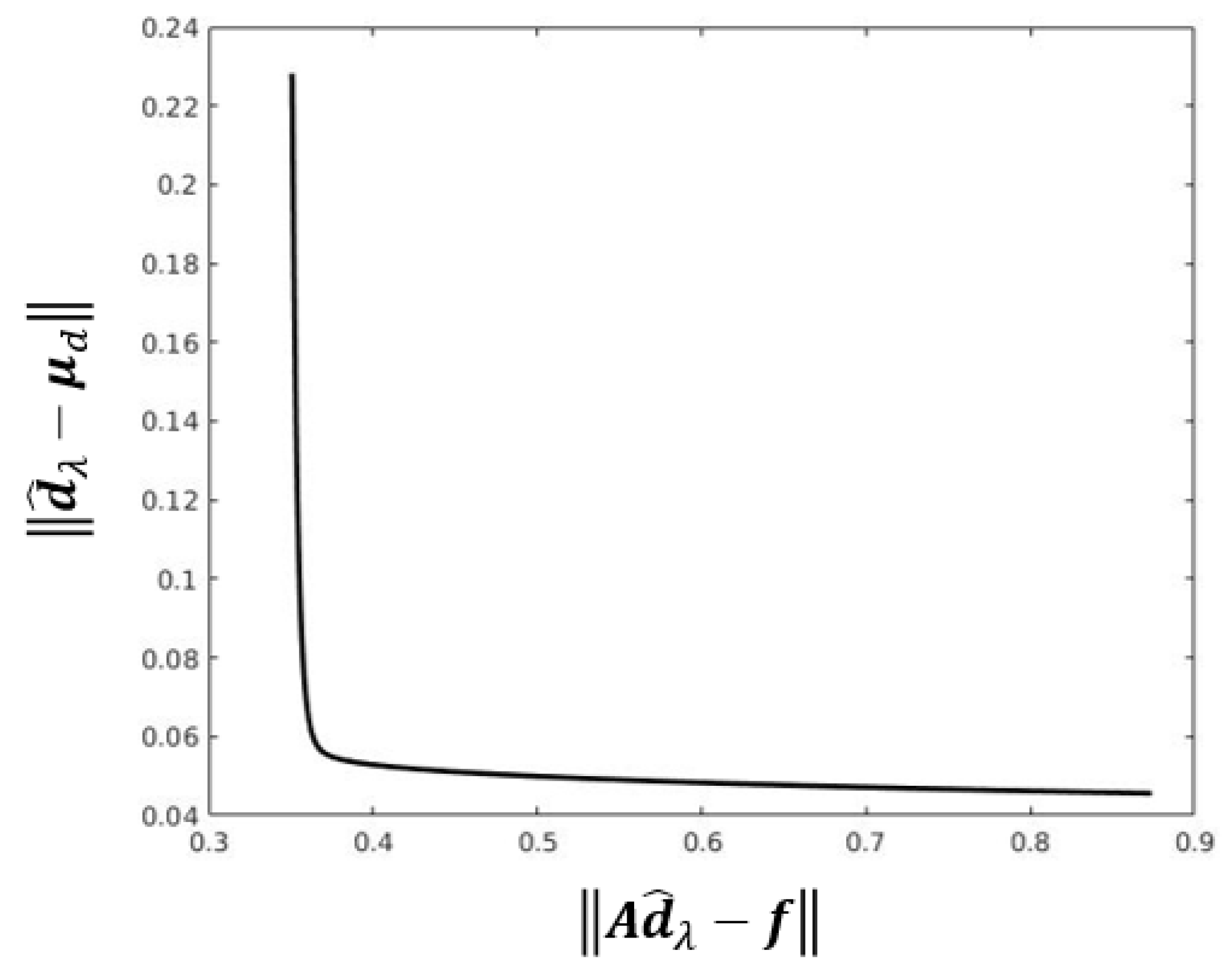
The L-curve method is a graphical procedure. The plot of the solution norm versus the residual norm displays an “L-shape” with a corner point, which corresponds to the desired regularization parameter. Koch and Kusche [32] demonstrated that the relative weighting between different observation types, as well as the regularization parameter, could be determined simultaneously by VCE. The prior information is added and regarded as an additional observation technique, and thus the regularization parameter can be interpreted as an additional variance component. However, in this case, the prior information is required to be of random character [32]. In most of the regional gravity modeling studies, a background model serves as prior information. In this case, the prior information has no random character, and the regularization parameter generated by VCE is not reliable [59]. Lieb [27] presented a case that shows the instability of VCE. Naeimi [60] showed that VCE delivers larger geoid RMS errors than the L-curve method, based on GRACE and GOCE data.
As VCE does not guarantee a reliable regularization solution, and the L-curve method (or other conventional regularization methods) cannot weight heterogeneous observations [61], the purpose of this paper is to combine VCE and the L-curve method to improve the stability and reliability of the gravity solutions. The idea of combining VCE for weighting different data sets only, and a method for determining the regularization parameter was introduced in the Section “future work” of both works in [59,60], but have not yet been applied in any further publications. The study in this manuscript is also inspired by the authors of [62,63]; the formal combines VCE for VLBI intra-technique combination and GCV for regularization; the latter combines a U-curve method for determining the regularization parameter and discriminant function minimization (DFM) for estimating the relative weighting between GPS and InSAR data. Our novel contribution focus on applying this idea for combining heterogeneous observations in regional gravity field modeling. Thus, we introduce and discuss in this paper two methods that combine VCE for determining the relative weighting between different observation types and the L-curve method for determining the regularization parameter, denoted as “VCE-Lc” and “Lc-VCE”, depending on the order of the applied procedures. Numerical experiments are carried out to compare their performance to the original L-curve method and VCE.
This work is organized as follows. Section 2 presents the fundamental concepts of SRBFs, different types of gravitational functionals, and their adapted basis functions. The parameter estimation, the Gauss–Markov model as well as the combination model are also introduced. Section 3 is dedicated to the regularization method, the L-curve method, VCE, and the two proposed combination methods. In Section 4, the study area, the data used in this study, and the model configuration are explained. Section 5 discusses the results. The performance of these four regularization methods is compared. Finally, the summary and conclusions are given in Section 6.

2. Regional Gravity Field Modelling Using SRBF

In general, a spherical basis function B ( x , x k ) related to a point P k with position vector x k on a sphere Ω R with radius R and an observation point P with position vector x can be expressed by
B ( x , x k ) = n = 0 2 n + 1 4 π R r n + 1 B n P n ( r T r k )
Ref. [4], with x = r · r = r · [ cos ϕ cos λ , cos ϕ sin λ , sin ϕ ] T , where λ is the spherical longitude, ϕ is the spherical latitude, x k = R · r k , P n is the Legendre polynomial of degree n, and B n is the Legendre coefficient which specifies the shape of the SRBF. When B n = 1 for all n, B ( x , x k ) represents the Dirac delta function, which has ideal spatial localization. With the spherical basis function (1), a harmonic signal F ( x ) given on the sphere Ω R or in the exterior space of Ω R , can be described as
F ( x ) = k = 1 K d k B ( x , x k ) ,
where K is the number of basis functions. The unknown coefficients d k can be evaluated from the observations. As will be shown in the following subsection, using these coefficients, any functional of F ( x ) can be described.

2.1. Gravity Representations

Various functionals can be derived from the gravitational potential V or from the disturbing potential T based on field transformations. The corresponding kernels can be derived from the definition (1) of the basis functions, and are listed in Table 1.
Disturbing potential: The disturbing potential T is defined as the difference between the gravity potential W and the normal gravity potential U,
T = W U ,
where the latter is the potential related to the level ellipsoid. The gravity potential W consists of two parts: the gravitational potential V and the centrifugal potential Z, i.e.,
W = V + Z .
Combining Equation (3) and Equation (4) yields [2]
T = V U + Z .
The disturbing potential T can be represented by
T ( x ) = k = 1 K d k B ( x , x k ) .
Gravitational potential difference: The satellite gravity field mission Gravity Recovery and Climate Experiment (GRACE) [64] consists of two satellites A and B. The main observable is the exact separation distance between the two satellites and its rate of change [65]. Several GRACE products exist (level 0 to level 2) [66,67]; the gravitational potential V can be computed from the level 2 products. In many studies (see, e.g., [20,27,60,68]), the differences between the gravitational potential values V of A and B are used as observations Δ V , i.e., Δ V ( x A , x B ) = V ( x A ) V ( x B ) . Including the measurement error e, the observation equation reads
Δ V ( x A , x B ) + e ( x A , x B ) = V ( x A ) V ( x B ) + e ( x A , x B ) = k = 1 K d k B ( x A , x B , x k ) .
Gravity disturbance: The gravity disturbance is used in airborne and terrestrial gravity field determination. The gravity disturbance vector δ g is expressed as the gradient of the disturbing potential T
δ g = T x , T y , T z T = grad T .
In spherical approximation, the magnitude of the gravity disturbance can be written as
δ g = T r = T r ,
its observation equation reads
δ g ( x ) + e ( x ) = k = 1 K d k B r ( x , x k ) .
Gravity gradient: Equipped with a 3-axis gradiometer, the satellite mission Gravity Field and Steady-State Ocean Circulation Explorer (GOCE) [69] observed the gravity gradients V a b with a , b { x , y , z } , i.e., all second-order derivatives of the gravitational potential V
V = V x x V x y V x z V y x V y y V y z V z x V z y V z z
with V x y = V y x , V x z = V z x , V y z = V z y and trace V = 0 due to the Laplacian differential equation. The observation data of GOCE used in this study are simulated as the radial component V r r = 2 V r 2 , and the observation equation reads
V r r ( x ) + e ( x ) = k = 1 K d k B r r ( x , x k ) .
For each type of gravitational functional, the adapted basis functions are derived by the zeroth, first, or second order derivatives of Equation (1), and they are listed in Table 1. Basis functions adapted to other functionals of the disturbing potential which are not used here can be found in [20,27,70].

2.2. Types of Spherical Radial Basis Functions

Different types of SRBFs can be found among others in [4,68]; the frequently used types include the Shannon function, the Blackman function, the cubic polynomial (CuP) function, and the Poisson function. Two types of band-limited SRBFs are used in this work, one without smoothing features (Shannon function), i.e., their shape coefficients (Legendre coefficients) equal to 1 for all frequencies within a certain bandwidth, and the other one with smoothing features (CuP function).
The Shannon function has the simplest representation; its Legendre coefficients are given by
B n = 1 for n [ 0 , N m a x ] 0 else
In case of the CuP function, the Legendre coefficients are given by a cubic polynomial, namely,
B n = ( 1 n N m a x ) 2 ( 1 + 2 n N m a x ) for n [ 0 , N m a x ] 0 else
N m a x is a certain degree to which the SRBFs are expanded, representing the cut-off degree. These two functions for N m a x = 255 are plotted in Figure 1, the top sub-plot and the bottom one visualize the characteristics in the spatial and the spectral domain, respectively. In the spatial domain, the Shannon function shows the sharper transition but also the stronger oscillations compared to the CuP function. In the spectral domain, the Shannon function is characterized by its exact band limitation without any smoothing features. The CuP function, however, has a smoothing decay. In this study, we apply both the Shannon function and the CuP function in the same experiments to test the performance of our proposed regularization methods.

2.3. Parameter Estimation

To determine the unknown coefficients d k in Equation (2), parameter estimation [36] is used in this study. This process allows the combination of different types of observations with varying resolutions, accuracies and distributions [71].

2.3.1. Gauss–Markov Model

For one single observation F ( x ) , the observation equation reads
F ( x ) + e ( x ) = k = 1 K d k B ( x , x k ) ,
B ( x , x k ) represents the adapted SRBFs as listed in Table 1. Collecting the observations F ( x 1 ) , F ( x 2 ) , …, F ( x n ) in the n × 1 observation vector f , the Gauss–Markov model
f + e = Ad ( deterministic part ) with D ( f ) = σ 2 P 1 ( stochastic part )
can be set up. In the deterministic part, e = [ e ( x 1 ) , e ( x 2 ) , , e ( x n ) ] T is the n × 1 vector of the observation errors and A = [ B ( x , x k ) ] is the n × K design matrix containing the corresponding basis functions. In the stochastic part, D ( f ) is the n × n covariance matrix of the observation vector f with σ 2 being the unknown variance factor and P being the given positive definite weight matrix.
Due to the three reasons mentioned in the introduction, namely, (1) the number of unknowns related to the basis functions, (2) data gaps, and (3) the downward continuation, the normal equation matrix N = A T P A is ill-posed or even singular. For handling this problem, we introduce an additional linear model
μ d + e d = d with D ( μ d ) = σ d 2 P d 1
as prior information. μ d is the K × 1 expectation vector of the coefficient vector d , e d is the corresponding error vector, and D ( μ d ) is the K × K covariance matrix of the prior information with σ d 2 the unknown variance factor and P d the positive definite weight matrix. Combining the two models (16) and (17) yields the extended linear model
f μ d + e e d = A I d with D f μ d = σ 2 P 1 0 0 0 + σ d 2 0 0 0 P d 1
Now the least-squares adjustment can be applied and leads to the normal equations
1 σ 2 A T P A + 1 σ d 2 P d d ^ = 1 σ 2 A T P f + 1 σ d 2 P d μ d
The variance factors σ 2 and σ d 2 can either be chosen or estimated within a VCE, and the solution reads
d ^ = ( A T P A + λ P d ) 1 ( A T P f + λ P d μ d )
D ( d ^ ) = σ 2 ( A T P A + λ P d ) 1 ,
wherein λ = σ 2 / σ d 2 can be interpreted as the regularization parameter, see [4,32]. When μ d is set to the zero vector, Equation (20) reduces to the Tikhonov regularization, and the regularization parameter λ can be determined by the L-curve method.

2.3.2. Combination Model

To combine different types of heterogeneous data sets for regional gravity field modeling, combination model (CM) needs to be set up (see, e.g., [4,32]). In general, let f l with l = 1 , , L be the observation vector of the l t h observation technique, such as f l = [ F l ( x 1 ) , F l ( x 2 ) , , F l ( x n l ) ] T , e l and A l are the corresponding error vector and the design matrix. Note that for different techniques, the data are observed as different gravitational functionals and thus, the adapted SRBFs as discussed in the Section 2.1 must be applied accordingly, A l = [ B l ( x , x k ) ] . For the combination of the L observation techniques, an extended Gauss–Markov model can be formulated by including the additional linear model (17) for the prior information
f 1 f 2 f L μ d + e 1 e 2 e L e d = A 1 A 2 A L I · d with D f 1 f 2 f L μ d = σ 1 2 P 1 1 0 0 0 0 σ 2 2 P 2 1 0 σ L 2 P L 1 0 0 0 0 σ d 2 P d 1
Ref. [27], where P l is the n l × n l positive definite weight matrix of the lth observation technique.
Applying the least-squares method to Equation (22), the extended normal equations read
l = 1 L ( 1 σ l 2 A l T P l A l ) + 1 σ d 2 P d d ^ = l = 1 L ( 1 σ l 2 A l T P l f l ) + 1 σ d 2 P d μ d .
The values for the variance factors can either be chosen or estimated by VCE (refer to Section 3.2). Consequently, the solution of Equation (23) reads
d ^ = l = 1 L ( 1 σ l 2 A l T P l A l ) + 1 σ d 2 P d 1 l = 1 L ( 1 σ l 2 A l T P l f l ) + 1 σ d 2 P d μ d .
The covariance matrix of the unknown parameter vectors reads
D ( d ^ ) = l = 1 L ( 1 σ l 2 A l T P l A l ) + 1 σ d 2 P d 1 .
Equation (24) can be rewritten as
d ^ = l = 1 L ( ω l A l T P l A l ) + λ P d 1 l = 1 L ω l A l T P l f l + λ P d μ d ,
such that λ = σ ^ 1 2 / σ ^ d 2 is the regularization parameter, and the factors ω 1 = σ ^ 1 2 / σ ^ 1 2 = 1 , ω 2 = σ ^ 1 2 / σ ^ 2 2 , , ω L = σ ^ 1 2 / σ ^ L 2 express the relative weights of the observation vector f l with respect to f 1 .

3. Determination of the Regularization Parameter

A critical question of regularization is the selection of an appropriate regularization parameter λ [72]. In the following, the L-curve method and the VCE will be explained in more detail. Finally, two new proposed methods are presented as combinations of VCE and the L-curve method.

3.1. L-Curve Method

The L-curve is a graphical procedure for regularization [28,33,34,73]. The norm of the regularized solution d ^ λ μ d is plotted against the norm of the residuals e ^ = A d ^ λ f by changing the numerical value for the regularization parameter λ . Moreover, the plot shows a typical L-curve behavior, i.e., it looks like the capital letter “L” (see Figure 2). The corner point in this L-shaped curve means a compromise of the minimization of the solution norm (which measures the regularity of the solution) and the residual norm (which quantifies the quality of fit to the given data), and thus can be interpreted as the “best fit” point that corresponds to the desired regularization parameter.
It should be mentioned that if the L-curve method is to be applied when different types of observations are combined, the relative weights ω l in Equation (24) need to be chosen. However, as it is not possible to know the accurate weights, the solution delivered by the L-curve method alone is, thus, not reliable.

3.2. Variance Component Estimation

Variance component estimation not only estimates the relative weighting between each data set but also determines the regularization parameter simultaneously. The variance components are estimated by an iterative process [20,32]. It starts from initial values for σ l 2 , σ d 2 , and ends in the convergence point. The estimations read
σ ^ l 2 = e ^ l T P l e ^ l r l σ ^ d 2 = e ^ d T P d e ^ d r d
where the residual vectors e ^ l and e ^ d are given as
e ^ l = A l d ^ f l e ^ d = d ^ μ d
and r l , r d are the partial redundancies, which are the contributions of the observations f l and the prior information μ d to the overall redundancy of Equation (22). The redundancy numbers r l , r d are computed following Koch and Kusche [32],
r l = n l trace ( 1 σ l 2 A l T P l A l N 1 ) r μ = K trace ( 1 σ d 2 P d N 1 )
where n l denotes the number of observations in the l t h data set, K is the number of coefficients, and
N = l = 1 L ( 1 σ l 2 A l T P l A l ) + 1 σ d 2 P d .
Starting with initial values for σ l 2 , σ d 2 , an initial solution for d ^ can be calculated, and it leads to the new estimations for σ ^ l 2 , σ ^ d 2 in Equation (27). The procedure iterates until the convergence point is reached.
As in the model represented by Equation (17) the prior information is regarded as an additional type of noisy observation, μ d is expected to be of stochastic character. However, when the background model serves as prior information, μ d is a deterministic vector. Consequently, e d = d μ d is also deterministic, and the requirements for the Equation (17) are in fact not fulfilled. Thus, in this case the regularization parameter λ generated by VCE is not reliable.

3.3. Combination of VCE and the L-Curve Method

To overcome the drawbacks in the L-curve method and in the VCE for combining heterogenous observations, two methods are proposed and applied in this study, namely, VCE-Lc and Lc-VCE.

3.3.1. VCE-Lc

Figure 3 illustrates the procedure of the VCE-Lc. In the first step, the VCE is applied to determine the relative weights between the observation types. This step gives the relative weighting factors ω l , and a regularization parameter λ VCE simultaneously, after the iteration converges. In the second step, the weighting factors ω l are kept, but the regularization parameter λ VCE is not used. Instead, a new regularization parameter is regenerated using the L-curve method. The corner point in the plot of the regularized solution norm d ^ λ μ d P d against the the residual norm e ^ = A d ^ λ f P corresponds to the new regularization parameter. In this case, the L-curve method is applied based on the variance factors σ ^ l 2 of each observation type generated by VCE. The corner point in Figure 2 corresponds to the new regularization parameter λ L-curve .
Thus, the final solution is computed using Equation (26) with the weights ω l from VCE and the new regularization parameter λ L-curve from the L-curve criterion.

3.3.2. Lc-VCE

Figure 4 illustrates the procedure of the Lc-VCE. In contrast to the VCE-Lc, in the Lc-VCE the L-curve method is applied first based on chosen values for the relative weights ω l in Equation (24). A regularization parameter λ L-curve is obtained in the first step, and it is used for defining the value of σ d 2 in the variance component estimation.
In the second step, the VCE is applied with initial values σ 1 2 = σ 2 2 = = σ L 2 and σ d 2 = σ 1 2 / λ L-curve . After each iteration within the VCE, the value of σ d 2 is set to σ 1 2 / λ L-curve again, with the new value of σ 1 2 obtained in this iteration. In this case, the regularization parameter λ calculated from the L-curve method will be kept, but the relative weighting factors ω l are recomputed in each iteration step. The final solution is computed using Equation (26) with the relative weights ω l and the regularization parameter λ L-curve .
It is worth clarifying that the solution obtained from the Lc-VCE is not unique. Due to the fact that the regularization parameter λ L-curve is fixed during VCE, the results change when λ L-curve refers to different observation techniques. To be more specific, as already mentioned in the last paragraph, the value of σ d 2 is set to σ 1 2 / λ L-curve after each iteration. Thus, the value of σ d 2 changes by setting different observation types as σ 1 2 , and the results of Equation (24) change, consequently.
To summarize, the purpose of these two proposed methods is to benefit from the L-curve method and VCE, and thus to overcome the drawbacks when using each method individually. VCE-Lc fixes the relative weights of each observation technique first and tries to find a “best fit” regularization parameter, whereas Lc-VCE fixes the regularization parameter first and then tries to find the relative weights for each observation technique.

4. Numerical Investigation

4.1. Data Description

The data used in this study are provided by the ICCT (Inter-Commission Committee on Theory) Joint Study Group (JSG) 0.3 “Comparison of current methodologies in regional gravity field modelling”, part of the IAG (International Association of Geodesy) programme running from 2011 to 2015. The observation data are simulated from the Earth Gravitational Model EGM2008 [74] and are provided along with simulated observation noise. In this study, all observations are simulated in the sense of disturbing gravity field quantities, i.e., functionals of the disturbing potential T: disturbing potential differences Δ T for GRACE, the first order radial derivatives T r for the terrestrial and airborne observations as well as the second order radial derivatives T r r for GOCE. The standard deviations of the given white noise are 8 · 10 4 m 2 / s 2 for GRACE, 10 mE for GOCE, 0.01 mGal for the terrestrial data and 1 mGal for the airborne data. The study area chosen here is “Europe”, where the validation data are also simulated from the EGM2008 and provided on geographic grid points in terms of disturbing potential values T.
Figure 5 illustrates the available observation data as well as the validation data. The two validation areas are presented with black rectangles: the larger area (Synthesis Data I) has a spatial resolution of 30 × 30 and is simulated with a maximum degree of 250; the smaller area (Synthesis Data II) has a spatial resolution of 5 × 5 and with a maximum degree of 2190. Four types of observations are included:
  • GRACE data: provided along the real satellite orbits of GRACE (green tracks in Figure 5), with a time span of one month.
  • GOCE data: provided along the real satellite orbits of GOCE (red tracks), covering a full repeat cycle of 61 days.
  • Terrestrial data: provided in a regular grid on the surface of the topography (DTM2006.0 [75]) with two different resolutions: one over an area of 20 × 30 (latitude × longitude) with a grid spacing of 30’ (blue dots) and the other one over an inner area of 6 × 10 with a grid spacing of 5’ (yellow highlighted area).
  • Airborne data: provided on two different flight tracks: one over the Adriatic Sea (magenta striped area) and the other one over Corsica connecting Southern Europe with Northern Africa (cyan striped area).
This study uses simulated data to take advantage of the availability of validation data. As this is a conceptual study to compare different methods, it is important to have an accurate validation data serving as the “true value” so that the gravity modeling result from each method can be evaluated and compared. Although validation when using real data is also possible, e.g., by comparing to GNSS/leveling data or to existing regional gravity models in the same region, the accuracy of the validation data then needs to be assessed beforehand.

4.2. Model Configuration

A Remove–Compute–Restore approach [76,77] is applied in this study, i.e., from each type of observation, the background model EGM2008 up to spherical harmonic degree 60 is removed and restored in the synthesis step. The background model serves additionally as prior information, and thus the vector d of the unknown coefficients contains the gravity information referring to a reference field (background model) up to degree and order 60. Koch and Kusche [32] pointed out that in this case, the expectation vector μ d can be set to the zero vector [4,27]. We assume that the coefficients have the same accuracy and are uncorrelated; thus, P d = I , where I denotes the identity matrix. Further, we set P l = I by assuming the measurement errors to be uncorrelated and the same type of observations to have the same accuracy. These assumptions are commonly used in the existing publications for both simulated and real data, since it is usually difficult to acquire the realistic full error variance-covariance matrix, and examples can be found in, e.g., [27,57,58].
As discussed in Section 3.1, the values of σ l 2 need to be chosen beforehand for the L-curve method. In studies where different observation types are involved, one might conduct an analysis on the relative weighting between the data sets in order to apply the L-curve method. Thus, in this study, empirically chosen values of σ l 2 are used for each observation type to have a more realistic result for the L-curve method. Lieb et al. [20] pointed out that the variance factors σ l 2 depend on the measurement accuracy, but also on the number, the spectral resolution, and the spatial distribution of the data. By using only the noise levels of each data set for calculating the variance factors, the σ l 2 values should be 0.64 · 10 6 for the GRACE data, 10 22 for the GOCE data, 10 10 for the airborne data, and 10 14 for the terrestrial data. However, Lieb (2017) showed that the airborne and terrestrial data are less sensitive in the low-frequency part, and their weights could degrade up to six orders of magnitude when the maximum degree of expansion is low. Taking both factors into consideration, the values of σ l 2 are chosen as 10 6 for the GRACE data, 10 22 for the GOCE data, and 10 8 for the terrestrial data and the airborne data in this study. It is worth mentioning that these values of σ l 2 are only approximations, and they are a choice for applying the L-curve method when VCE is not considered. Moreover, the purpose of this study is not to compare between the L-curve method and VCE, but to compare the two proposed methods with using the L-curve method or VCE individually. The results for the L-curve method without relative weights (equal weighting between each data set) are also presented in Section 5.1 as a comparison scenario.
In this study, different observation types are combined in a “one-level” manner, which is also applied in, e.g., [20,58,68]. The relative weights indicate the contributions of different observation types [20]. Another way for combining different types of observations is the spectral combination (see, e.g., in [78,79,80]), where the (spectral) weights depend on the spectral degree. The spectral weights at each degree can be incorporated into the (kernel) functions [79], and studies about how to find the optimal kernels can be found in, e.g., [80,81]. However, details about the spectral combination technique would go beyond the scope of this study.
Figure 6 presents the computation area Ω C , the observation area Ω O , as well as the investigation area Ω I . The computation area Ω C should be larger than the observation area Ω O , due to the oscillations of the SRBFs. The observation area Ω O should be larger than the investigation area Ω I , because the unknown coefficients d k cannot be accurately estimated in the border of the observation area Ω O . Thus, Ω I Ω O Ω C , and detailed explanations for this extension can be found in [27,60]. In the analysis step, we estimate the vector d ^ of the unknown coefficients d k related to the grid points P k within the computation area Ω C , from the measurements available within the area Ω O . In the following synthesis step, these coefficients are used for calculating the output gravity functional within the area Ω I . It has to be mentioned that the points P k within the computation area Ω C are defined by a Reuter grid [82]. The Reuter’s algorithm generates a system of homogeneous points on the sphere [22]. Margins η between the computation area Ω C and the observation area Ω O as well as between the observation area Ω O and the investigation area Ω I are chosen equally, and they have to be defined to minimize edge effects in the computation process [20]. In this study, we conducted the experiments using different margin sizes (from 1 to 4 ), and the ones (values given in Section 5) which result in the smallest difference between the estimated disturbing potential and the validation data are finally chosen.
The aforementioned four methods for choosing the regularization parameter, i.e., (1) L-curve method, (2) VCE, (3) VCE-Lc, and (4) Lc-VCE, are applied to six groups of data sets, respectively. The types of observations involved in the six study cases as well as the corresponding validation data for each study case are listed in Table 2. These six groups cover the possible combination among the four data types, to make sure that the comparisons of these four methods are conducted in different data combination scenario. The computed disturbing potential T c is compared with the corresponding validation data T v and assessed following two criteria:
  • Root mean square error (RMS) of the computed disturbing potential T c with respect to the validation data T v over the investigation area Ω I
    RMS = n points ( T v T c ) 2 n points
    where n points is the number of points in the validation data.
  • Correlation coefficient between the estimated coefficients d k collected in the vector d ^ and the validation data T v . It has to be clarified that the estimated coefficients d k and the validation data T v are located at different points, and an interpolation is conducted to transit d k to the grid of the validation data.
    The reason that this correlation can be used as a criterion is that the coefficients d k reflect the energy of the gravity field at their locations. On a sphere embedded in a three-dimensional space, the energy of a signal F ( x ) can be expressed by
    E = Ω R | F ( x ) | 2 d Ω R .
    Combining Equation (2) with Equation (32), it yields
    E = Ω R | k = 1 K d k B ( x , x k ) | 2 d Ω R = k = 1 K d k i = 1 K d i Ω R B ( x , x k ) B ( x , x i ) d Ω R .
    By inserting the series expansion of the SRBFs (Equation 1) on Ω R to Equation (33) and applying the addition theorem (details about the equation manipulation can be found in [27]), the energy contribution E k ( k = 1 , 2 , , K ) at location x k is given as
    E k = d k i = 1 K d i n = 0 N m a x 2 n + 1 4 π B n 2 P n ( r i T r k ) .
    When N m a x goes to , and B n =1 for all n, i.e., in the case of the Dirac delta function, E k = d k 2 . In the case of SRBFs where N m a x , and B n is not necessarily equal to 1, the relation E k = d k 2 is only approximately valid. However, a higher correlation between the coefficients d k and the validation data still indicates a better representation of the gravity signal. The same criterion is used as a quality measure by [23,25].

5. Results

The experiments are carried out using the Shannon function for both analysis and synthesis. However, to test the performance of these four methods when a smoothing SRBF is used, the same experiments are also applied using the CuP function for analysis and synthesis as a comparison scenario. The maximum degree in the expansion in terms of SRBF is chosen based on the spatial resolution of the observations [20,57], and it is set to N m a x = 250 for the study cases A and B; N m a x = 400 for the study cases C and D; N m a x = 2190 for the study cases E; and N m a x = 1050 for the study case F. The margin η between the different areas (Figure 6) is chosen to be 4 for the study cases A, B, C, and D, and 2 for the study cases E and F.
For the sake of brevity, only the results of two study cases (case A in Table 3 and case F in Table 4) are detailed here. Results from the case A and the case F clearly show the drawbacks of VCE and the L-curve method, respectively. However, results obtained from all study cases, including the RMS errors and the correlations between the estimated coefficients d k and the validation data T v of each method are summarized in the Table 5 and Table 6, respectively. The results when using the CuP function are listed in the Table 7 and Table 8.

5.1. Results Using the Shannon Function

5.1.1. Study Case A

GRACE and GOCE observations are combined. Four solutions are estimated according to the aforementioned four methods for determining the regularization parameter. For each solution, the RMS error as well as the correlation between the estimated coefficients d k and the validation data T v are listed in Table 3. Two scenarios are considered, depending on how the relative weights ω l (or the variance factors σ l 2 ) between each observation type are chosen in the L-curve method and Lc-VCE. In the first scenario, the relative weights ω l are chosen empirically (see Section 4.2). The lowest RMS error is obtained from the VCE-Lc which is 4.59 m 2 / s 2 . This method also delivers the highest correlation between the estimated coefficients d k and the validation data. Lc-VCE gives the second best RMS value which is 4.61 m 2 / s 2 (Referring to Section 3.3.2, the solution obtained from Lc-VCE is not unique, and the results listed here for Lc-VCE are always the best ones, i.e., the solution which gives the lowest RMS and largest correlation). For each solution, the estimated coefficients d k , the calculated disturbing potential T c , as well as its difference to the validation data are plotted in Figure 7. VCE gives the smallest correlation and the largest difference compared to the validation data. The RMS error obtained from VCE is 7.84 m 2 / s 2 , which is ~70% larger than those obtained from VCE-Lc or Lc-VCE.
In reality, it is difficult to choose the empirical weights between different observation types accurately, as the accuracy of different observation types is not available. As listed in Table 3, in the second scenario, when no relative weights are applied (equal weighting between data sets), the performance of the L-curve method decreases, with a 56% increase in RMS error. This increase demonstrates the importance of accurately weighting different data sets. The result obtained from the Lc-VCE also decreases slightly, with the RMS error increases from 4.61 m 2 / s 2 to 5.17 m 2 / s 2 . In this scenario, VCE-Lc and Lc-VCE still deliver the lowest and second lowest RMS error, respectively. The same order applies to the correlation between the estimated coefficients d k and the validation data. The RMS error from VCE-Lc is 36% and 41% smaller than that delivered by the L-curve method and VCE, respectively. The RMS error from Lc-VCE is 28% and 34% smaller than that delivered by the L-curve method and VCE, respectively. VCE still gives the largest RMS error as well as the smallest correlation, which proves that VCE does not determine the regularization parameter as successful as the L-curve method, since it gives a worse result than the L-curve method which is based on an equal weighting between each observation type.

5.1.2. Study Case F

In case F, four data sets (GRACE, GOCE, the terrestrial II, and the airborne I observations) are combined. Compared to the study case A, the results in the study case F (listed in Table 4) show a general improvement, in terms of both the two criteria. When the relative weights ω l are chosen empirically (see Section 4.2), VCE-Lc provides the smallest RMS error 0.84 m 2 / s 2 , followed by the Lc-VCE. The same order applies to the correlation between the estimated coefficients d k and the validation data. The L-curve method delivers the largest RMS value with 0.91 m 2 / s 2 , as well as the smallest correlation. It shows that the empirically chosen relative weights between different observation types are not accurate, and it is necessary to estimate the weights with VCE. For each solution, the estimated coefficients d k , the calculated disturbing potential T c as well as its difference to the validation data are plotted in Figure 8. It shows that the L-curve method delivers the largest difference compared to the validation data.
When no relative weights are applied (equal weighting), the performance of the L-curve method decreases, with a 61% increase in RMS error. Further, in this case, it delivers the worst results, with an RMS error 75% larger than the ones obtained by VCE-Lc or Lc-VCE. It shows that when more types of observation are involved, combining each observation technique with a relative weight becomes even more important. VCE-Lc again delivers the smallest RMS error as well as the highest correlation, followed by Lc-VCE.

5.1.3. Results of All Six Cases

For all the six study cases, the RMS error obtained from each regularization method using the Shannon function are summarized in Table 5, the correlations between the estimated coefficients and the validation data are listed in Table 6.
Comparing to VCE, the two proposed methods, VCE-Lc and Lc-VCE, give smaller RMS errors as well as larger correlations in all the six study cases. In study cases A and B, the differences between the results delivered by VCE and the ones from the proposed methods are large, i.e., the RMS errors obtained from the VCE-Lc or Lc-VCE are 41% and 61% smaller than the ones obtained by VCE in case A and B, respectively. It indicates that VCE is unable to regularize the solutions properly in these two cases. In case A, when GRACE and GOCE are combined, the downward continuation of the satellite data requires strong regularization. VCE cannot provide sufficient regularization in this case. This result coincides with the conclusion drawn by Naeimi [60], who showed that VCE gives similar RMS errors as the L-curve method at the orbit level, but it is not able to provide sufficient regularization at the Earth surface for the regional solutions based on satellite data. Moreover, the high errors in the satellite data could be another reason for the large RMS error from VCE in this study case. And if the data errors are reduced by two orders of magnitude, the RMS error delivered by VCE-Lc or Lc-VCE becomes 22% smaller than that from VCE in case A. In case B, when the GRACE data are combined with the two airborne data sets, large data gaps exist along the study area, which also requires strong regularization. As we have mentioned in the Introduction, data gaps and the downward continuation are two of the major reasons why regularization is needed in regional gravity field modeling. Thus, VCE is also not able to provide sufficient regularization in study case B due to both large data gaps and the downward continuation of the data. The study cases A and B could be two extreme cases, i.e., in realistic applications of regional gravity field modeling, usually not only satellite data are used, and data gaps will not be as large as in study case B. However, we present these two cases here to give a complete view for the comparisons of the four regularization methods in different combination scenarios.
In the other four cases, when the terrestrial data are included, and there are much less data gaps, the RMS errors obtained from VCE differ with VCE-Lc and Lc-VCE less. The RMS errors from the VCE-Lc decrease by 4%, 8%, 5%, and 0.4%, and the RMS errors from the Lc-VCE decrease by 4%, 7%, 4%, and 0.2% in study cases C, D, E, F, compared to the ones obtained from VCE. These results show a more unbiased view of the benefits of the two proposed approaches compared to VCE, in realistic applications when different regional gravity observations are involved. Although the improvements obtained by VCE-Lc or Lc-VCE compared to VCE are not as large as in the cases A and B, the two proposed methods still deliver smaller RMS errors and higher correlations in all the study cases.
The RMS errors from the VCE-Lc decrease by 0.7%, 4%, 2%, 8%, 4%, and 8%, and the RMS errors from the Lc-VCE decrease by 0.3%, 4%, 2%, 7%, 2%, and 8% compared to the ones from the L-curve method, in the six study cases. The improvements of the proposed methods compared to the L-curve method are not that large because the relative weights between different data sets were chosen empirically, with the knowledge of the data accuracy. In reality, the relative weights are not necessarily to be chosen accurately, especially when the accuracy of different real data sets is not available. Moreover, the results from the L-curve method heavily depend on the chosen relative weights. As shown in Section 5.1.1 and Section 5.1.2, if different data sets are combined without relative weights (equal weighting), the RMS error from VCE-Lc decreases by 36% and 43% compared to the L-curve method in case A and F, respectively. These results show that the empirically chosen weights are important for the L-curve method, and wrongly chosen weights will lead to unreliable modeling results. VCE-Lc not only reduces the RMS errors compared to the L-curve method, but it also avoids the need for determining empirical weights, and thus, avoids the effect of wrongly chosen weights.
As the results delivered by Lc-VCE also change slightly when different relative weights are chosen (see Section 5.1.1 and Section 5.1.2), it is worth mentioning that we have also conducted an iterative procedure for the Lc-VCE, which means applying the Lc-VCE repeatedly until the regularization parameter stays unchanged. At each iteration, the L-curve method is applied based on the relative weights obtained from the last VCE procedure. To be more specific, based on the relative weights obtained from the Lc-VCE, the L-curve method is applied again to generate the regularization parameter; VCE is then applied based on this regularization parameter to generate the relative weights, and the L-curve method is applied again, and so on. The L-curve method and VCE are applied successively until the regularization parameter and the relative weights do not change anymore. However, no significant improvements have been observed compared to the results delivered by the Lc-VCE; furthermore, this iterative procedure is time-consuming. Thus, we do not propose it in this paper.
To summarize, the two proposed methods improve the modeling results compared to using the L-curve method or VCE alone in all the six study cases. Among the two proposed methods, VCE-Lc delivers not only smaller RMS errors but also higher correlations than the Lc-VCE in five out of six study cases. Lc-VCE also shows good performance; however, the reference observation type in this method needs to be chosen carefully. Another advantage of using the VCE-Lc is that there is no need for determining the empirical weights in this approach, which is required in the L-curve method and Lc-VCE. Moreover, the results in terms of RMS value and correlation are consistent, i.e., the method which gives a smaller RMS error also delivers a larger correlation. However, the correlations differ much less than the RMS errors do between each method.

5.2. Results Using the CuP Function

Table 7 and Table 8 list the RMS values as well as the correlations between the estimated coefficients d k and the validation data T v of each method when the CuP function is used.
When the CuP function is used, the proposed two methods still always deliver better results than the L-curve method and VCE, in terms of both RMS value and correlation for all the six study cases. The RMS errors from the VCE-Lc decrease by 4%, 16%, 14%, 19%, 11%, and 0.05% compared to those obtained from VCE, and by 1%, 8%, 3%, 10%, 1%, and 4% compared to the results from the L-curve method, in the six study cases. The RMS errors from the Lc-VCE decrease by 4%, 16%, 13%, 19%, 10%, and 0.03% compared to those obtained from VCE, and by 1%, 8%, 3%, 10%, 1%, and 4% compared to the results from the L-curve method, in the six study cases. These results show that improvements are achieved in the proposed methods, no matter using SRBFs with or without smoothing features. VCE-Lc still performs the best among the four regularization methods. When the CuP function is used, the differences between VCE and VCE-Lc become smaller in terms of RMS error (especially in cases A and B) but larger in terms of correlation. This behavior is consistent with the publication [23], which demonstrated that the SRBFs with smoothing features have a built-in regularity. Naeimi [60] concluded that VCE should be used with SRBFs which have smoothing features (e.g., the CuP function), based on both simulated and real satellite observations. The results using the CuP function in this study show that even when using an SRBF with smoothing features, the proposed VCE-Lc and Lc-VCE can still achieve improvements compared to using VCE alone.

6. Summary and Conclusions

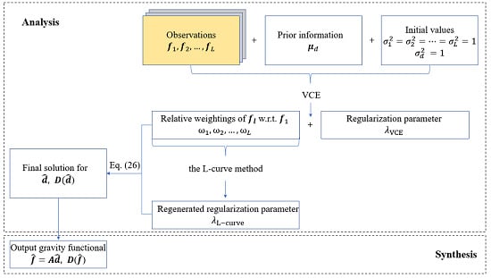
This study discusses the regularization methods when heterogeneous observations are to be combined in regional gravity field modeling. We analyze the drawbacks of the two traditional regularization methods, namely, the L-curve method and VCE. When the L-curve method is applied, the relative weights between different observation types need to be chosen beforehand, and the modeling results heavily depend on if the relative weights are chosen accurately. In VCE, the prior information is regarded to be another observation type and is required to be stochastic. However, in regional gravity modeling, the prior information is not stochastic, and in this case, the regularization parameter generated by VCE could be unreliable. We propose two “combined methods” which combine VCE and the L-curve method in such a way that the relative weights are estimated by VCE, but the regularization parameters are determined by the L-curve method. The two proposed methods differ in whether determining the relative weights between each observation type first (VCE-Lc) or the regularization parameter by the L-curve method first (Lc-VCE).
We compare the two proposed methods, VCE-Lc and Lc-VCE, with the L-curve method and VCE. Each method is applied to six groups of data sets with simulated satellite, terrestrial and airborne data in Europe, and the results are compared to the validation data with corresponding spatial and spectral resolutions. These data are simulated from EGM2008 and are provided by the IAG ICCT JSG 0.3, along with the simulated observation noise. The RMS error between the computed disturbing potential and the validation data, as well as the correlation between the estimated coefficients and the validation data are used as the comparison criteria. The investigation shows that the two proposed methods deliver smaller RMS errors and larger correlations than the L-curve method and VCE, in all the six study cases. In cases A and B, VCE fails to provide sufficient regularization due to large data gaps, the downward continuation, and high errors in the satellite data. In cases C–F, the RMS errors from VCE-Lc decrease by 4%, 8%, 5%, and 0.4%, respectively, compared to those obtained from VCE. The RMS errors from VCE-Lc decrease by 0.7%, 4%, 2%, 8%, 4%, and 8% compared to the results from the L-curve method (when the relative weights are chosen empirically), in the six study cases. However, when the relative weights are chosen inaccurately (e.g. equal weighting), the RMS error obtained by VCE-Lc reaches a value 43% smaller than that from the L-curve method. Among the four tested methods, the VCE-Lc gives the best results in terms of both RMS error and the correlation between the estimated coefficients and the validation data. Moreover, another advantage of using the VCE-Lc is that there is no need for determining the empirical weights beforehand, which is required in both the L-curve method and Lc-VCE.
We also carry out the same investigation using the CuP function, which has smoothing features as a comparison scenario. VCE-Lc and Lc-VCE still give the best and second best results in terms of both RMS error and the correlation. From our investigation, we conclude that VCE-Lc is the best choice among the applied methods for the determination of the regularization parameter when heterogeneous observations are to be combined, no matter using SRBFs with or without smoothing features.
In the future, a primary concern is to apply the newly devised methods using more types of SRBFs, so that the performance of different SRBFs can be compared while making sure that the differences in results are not coming from the regularization method. In addition, after validating the proposed methods with simulated data in this study, they have also been applied to real observations for the regional geoid modeling in Colorado, USA, within the “1 cm Geoid Experiment” [83]. The experiment was proposed within four scientific groups, namely, (1) the Global Geodetic Observing System (GGOS) Joint Working Group (JWG) 0.1.2, (2) the IAG JWG 2.2.2, (3) the IAG Sub-Commission (SC) 2.2, and (4) the ICCT JSG 0.15. We are currently preparing a related publication; the validation and comparison of different methodologies applied in this experiment can be found in [84].

Author Contributions

Conceptualization, Q.L.; Methodology, Q.L. and M.S.; Software, Q.L.; Validation, Q.L. and M.S.; Formal Analysis, Q.L.; Investigation, Q.L.; Resources, Q.L. and M.S.; Data Curation, Q.L.; Writing—Original Draft Preparation, Q.L.; Writing—Review and Editing, Q.L., M.S., R.P., and M.W.; Visualization, Q.L.; Supervision, M.S.; Project Administration, M.S. and R.P.; Funding Acquisition, M.S. and R.P. All authors have read and agreed to the published version of the manuscript.

Funding

This research was funded by Deutsche Forschungsgemeinschaft (DFG), grant number, SCHM 2433/11-1. The APC was funded by Institutional Open Access Program of the Technichal University of Munich (TUM).

Acknowledgments

This study was conducted in the framework of the project “Optimally combined regional geoid models for the realization of height systems in developing countries”, the authors would like to thank the German Research Foundation (DFG) for funding this project. We also acknowledge the ICCT Joint Study Group 0.3 for providing the data sets. We are grateful to Katrin Bentel for kindly providing support and the basic programme related to this work. Furthermore, the authors acknowledge the developers of the Generic Mapping Tool (GMT) mainly used for generating the figures in this work. The authors thank the editor and three reviewers for their comments that allowed them to improve this paper.

Conflicts of Interest

The authors declare no conflicts interest.

References

  1. Heiskanen, W.A.; Moritz, H. Physical Geodesy; San Francisco W. H. Freeman and Company: San Francisco, CA, USA, 1967; ISBN 978-3-211-33544-4. [Google Scholar]
  2. Hofmann-Wellenhof, B.; Moritz, H. Physical Geodesy; Springer-Verlag Wien: Vienna, Austria, 2005; ISBN 3-211-23584-1. [Google Scholar]
  3. Jekeli, C. Spline Representations of Functions on a Sphere for Geopotential Modeling; Technical Report; Ohio State University: Columbus, OH, USA, 2005. [Google Scholar]
  4. Schmidt, M.; Fengler, M.; Mayer-Gürr, T.; Eicker, A.; Kusche, J.; Sánchez, L.; Han, S.C. Regional gravity modeling in terms of spherical base functions. J. Geod. 2007, 81, 17–38. [Google Scholar] [CrossRef] [Green Version]
  5. Krarup, T. The method of least squares collocation. Stud. Geophys. Geod. 1970, 14, 107–109. [Google Scholar] [CrossRef]
  6. Moritz, H. Advanced Physical Geodesy; Herbert Wichmann Verlag: Kalsruhe, Germany, 1980; ISBN 978-3879071951. [Google Scholar]
  7. Pail, R.; Reguzzoni, M.; Sansó, F.; Kühtreiber, N. On the combination of global and local data in collocation theory. Stud. Geophys. Geod. 2010, 54, 195–218. [Google Scholar] [CrossRef]
  8. Rowlands, D.D.; Luthcke, S.; Klosko, S.; Lemoine, F.G.; Chinn, D.; McCarthy, J.; Cox, C.; Anderson, O. Resolving mass flux at high spatial and temporal resolution using GRACE intersatellite measurements. Geophys. Res. Lett. 2005, 32. [Google Scholar] [CrossRef]
  9. Rowlands, D.; Luthcke, S.; McCarthy, J.; Klosko, S.; Chinn, D.; Lemoine, F.; Boy, J.P.; Sabaka, T. Global mass flux solutions from GRACE: A comparison of parameter estimation strategies—Mass concentrations versus Stokes coefficients. J. Geophys. Res. Solid Earth 2010, 115. [Google Scholar] [CrossRef]
  10. Jacob, T.; Wahr, J.; Pfeffer, W.T.; Swenson, S. Recent contributions of glaciers and ice caps to sea level rise. Nature 2012, 482, 514–518. [Google Scholar] [CrossRef]
  11. Simons, F.J.; Dahlen, F.; Wieczorek, M.A. Spatiospectral concentration on a sphere. SIAM Rev. 2006, 48, 504–536. [Google Scholar] [CrossRef] [Green Version]
  12. Simons, F.J. Slepian functions and their use in signal estimation and spectral analysis. In Handbook of Geomathematics; Freeden, W., Nashed, Z.M., Sonar, T., Eds.; Springer: Berlin, Germany, 2009; pp. 891–923. [Google Scholar]
  13. Marchenko, A.N. Parameterization of the Earth’s Gravity Field: Point and Line Singularities; Lviv Astronomical and Geodetic Society: Lviv, Ukraine, 1998; ISBN 9785776346040. [Google Scholar]
  14. Holschneider, M.; Chambodut, A.; Mandea, M. From global to regional analysis of the magnetic field on the sphere using wavelet frames. Phys. Earth Planet. Inter. 2003, 135, 107–124. [Google Scholar] [CrossRef]
  15. Freeden, W.; Michel, V. Multiscale Potential Theory: With Applications to Geoscience; Birkhäuser: Basel, Switzerland, 2004; ISBN 978-1-4612-2048-0. [Google Scholar]
  16. Freeden, W.; Schreiner, M. Spherical Functions of Mathematical Geosciences: A Scalar, Vectorial, and Tensorial Setup; Springer Science & Business Media: Berlin, Germany, 2009; ISBN 978-3-642-09881-9. [Google Scholar]
  17. Freeden, W.; Gervens, T.; Schreiner, M. Constructive Approximation on the Sphere with Applications to Geomathematics; Oxford University Press on Demand: New York, NY, USA, 1998; ISBN 978-0198536826. [Google Scholar]
  18. Freeden, W. Multiscale Modelling of Spaceborne Geodata; Teubner: Stuttgart, Germany, 1999. [Google Scholar]
  19. Marchenko, A.N. Regional gravity field model from satellite altimetry, gravimetry, and GPS-leveling data in the Black Sea area. BOllettino Geod. Sci. Affin. LXII 2003, 4, 245–259. [Google Scholar]
  20. Lieb, V.; Schmidt, M.; Dettmering, D.; Börger, K. Combination of various observation techniques for regional modeling of the gravity field. J. Geophys. Res. Solid Earth 2016, 121, 3825–3845. [Google Scholar] [CrossRef]
  21. Li, X. Using radial basis functions in airborne gravimetry for local geoid improvement. J. Geod. 2018, 92, 471–485. [Google Scholar] [CrossRef]
  22. Wittwer, T. Regional Gravity Field Modelling with Radial Basis Functions. Ph.D. Thesis, Netherlands Geodetic Commission, Delft, The Netherlands, 2009. [Google Scholar]
  23. Naeimi, M.; Flury, J.; Brieden, P. On the regularization of regional gravity field solutions in spherical radial base functions. Geophys. J. Int. 2015, 202, 1041–1053. [Google Scholar] [CrossRef] [Green Version]
  24. Tenzer, R.; Klees, R. The choice of the spherical radial basis functions in local gravity field modeling. Stud. Geophys. Geod. 2008, 52, 287–304. [Google Scholar] [CrossRef] [Green Version]
  25. Bentel, K.; Schmidt, M.; Denby, C.R. Artifacts in regional gravity representations with spherical radial basis functions. J. Geod. Sci. 2013, 3, 173–187. [Google Scholar] [CrossRef]
  26. Eicker, A. Gravity field Refinement by Radial Basis Functions from In-Situ Satellite Data. Ph.D. Thesis, University of Bonn, Bonn, Germany, 2008. [Google Scholar]
  27. Lieb, V. Enhanced Regional Gravity Field Modeling from the Combination of Real Data via MRR. Ph.D. Thesis, Technische Universität München, Munich, Germany, 2017. [Google Scholar]
  28. Bouman, J. Quality of Regularization Methods. DEOS Report 98.2; Technical Report; Delft University Press: Delft, The Netherlands, 1998. [Google Scholar]
  29. Tikhonov, A.N.; Arsenin, V.I. Solutions of ill-posed Problems; Winston: Washington, DC, USA, 1977; ISBN 978-0470991244. [Google Scholar]
  30. Xu, P. Truncated SVD methods for discrete linear ill-posed problems. Geophys. J. Int. 1998, 135, 505–514. [Google Scholar] [CrossRef]
  31. Schuh, W.D. Tailored Numerical Solution Strategies for the Global Determination of the Earth’s Gravity Field; Technical Report; Technischen Universität Graz: Graz, Austria, 1996. [Google Scholar]
  32. Koch, K.R.; Kusche, J. Regularization of geopotential determination from satellite data by variance components. J. Geod. 2002, 76, 259–268. [Google Scholar] [CrossRef]
  33. Hansen, P.C. Truncated singular value decomposition solutions to discrete ill-posed problems with ill-determined numerical rank. SIAM J. Sci. Stat. Comput. 1990, 11, 503–518. [Google Scholar] [CrossRef]
  34. Hansen, P.C.; O’Leary, D.P. The use of the L-curve in the regularization of discrete ill-posed problems. SIAM J. Sci. Comput. 1993, 14, 1487–1503. [Google Scholar] [CrossRef]
  35. Grafarend, E.; Kleusberg, A.; Schaffrin, B. An introduction to the variance-covariance component estimation of Helmert type. Z. FüR Vermess. 1980, 105, 161–180. [Google Scholar]
  36. Koch, K.R. Parameter Estimation and Hypothesis Testing in Linear Models; Springer: Berlin/Heidelberg, Germany, 1999; ISBN 978-3-642-08461-4. [Google Scholar]
  37. Wahba, G. Spline Models for Observational Data; SIAM: Philadelphia, PA, USA, 1990; ISBN 978-0-89871-244-5. [Google Scholar]
  38. Haber, E. Numerical Strategies for the Solution of Inverse Problems. Ph.D. Thesis, The University of British Columbia, Vancouver, BC, Canada, 1997. [Google Scholar]
  39. Li, Y.; Oldenburg, D.W. Fast inversion of large-scale magnetic data using wavelet transforms and a logarithmic barrier method. Geophys. J. Int. 2003, 152, 251–265. [Google Scholar] [CrossRef] [Green Version]
  40. Liu, X. Global Gravity Field Recovery from Satellite-to-Satellite Tracking Data with the Acceleration Approach. Ph.D. Thesis, Technical University of Delft, Delft, The Netherlands, 2008. [Google Scholar]
  41. Van Loon, J. Functional and Stochastic Modelling of Satellite Gravity Data. Ph.D. Thesis, Technical University of Delft, Delft, The Netherlands, 2008. [Google Scholar]
  42. Akaike, H. Likelihood and the Bayes procedure. Trab. Estad. Investig. Oper. 1980, 31, 143–166. [Google Scholar] [CrossRef] [Green Version]
  43. Yabuki, T.; Matsu’Ura, M. Geodetic data inversion using a Bayesian information criterion for spatial distribution of fault slip. Geophys. J. Int. 1992, 109, 363–375. [Google Scholar] [CrossRef]
  44. Mitsuhata, Y.; Uchida, T.; Amano, H. 2.5-D inversion of frequency-domain electromagnetic data generated by a grounded-wire source. Geophysics 2002, 67, 1753–1768. [Google Scholar] [CrossRef]
  45. Fukahata, Y.; Nishitani, A.; Matsu’ura, M. Geodetic data inversion using ABIC to estimate slip history during one earthquake cycle with viscoelastic slip-response functions. Geophys. J. Int. 2004, 156, 140–153. [Google Scholar] [CrossRef] [Green Version]
  46. Liu, Y.; Fok, H.S.; Tenzer, R.; Chen, Q.; Chen, X. Akaike’s Bayesian Information Criterion for the Joint Inversion of Terrestrial Water Storage Using GPS Vertical Displacements, GRACE and GLDAS in Southwest China. Entropy 2019, 21, 664. [Google Scholar] [CrossRef] [Green Version]
  47. Wu, L. A parameter choice method for Tikhonov regularization. Electron. Trans. Numer. Anal. 2003, 16, 107–128. [Google Scholar]
  48. Ceccherini, S. Analytical determination of the regularization parameter in the retrieval of atmospheric vertical profiles. Opt. Lett. 2005, 30, 2554–2556. [Google Scholar] [CrossRef]
  49. Ridolfi, M.; Sgheri, L. Iterative approach to self-adapting and altitude-dependent regularization for atmospheric profile retrievals. Opt. Express 2011, 19, 26696–26709. [Google Scholar] [CrossRef]
  50. Albani, V.; De Cezaro, A.; Zubelli, J.P. On the Choice of the Tikhonov Regularization Parameter and the Discretization Level: A Discrepancy-Based Strategy. Inverse Probl. Imaging 2016, 10, 1–25. [Google Scholar] [CrossRef]
  51. Steck, T. Methods for determining regularization for atmospheric retrieval problems. Appl. Opt. 2002, 41, 1788–1797. [Google Scholar] [CrossRef]
  52. Farquharson, C.G.; Oldenburg, D.W. A comparison of automatic techniques for estimating the regularization parameter in non-linear inverse problems. Geophys. J. Int. 2004, 156, 411–425. [Google Scholar] [CrossRef] [Green Version]
  53. Xu, J.; Schreier, F.; Doicu, A.; Trautmann, T. Assessment of Tikhonov-type regularization methods for solving atmospheric inverse problems. J. Quant. Spectrosc. Radiat. Transf. 2016, 184, 274–286. [Google Scholar] [CrossRef] [Green Version]
  54. Ramillien, G.; Biancale, R.; Gratton, S.; Vasseur, X.; Bourgogne, S. GRACE-derived surface water mass anomalies by energy integral approach: Application to continental hydrology. J. Geod. 2011, 85, 313–328. [Google Scholar] [CrossRef]
  55. Xu, C.; Ding, K.; Cai, J.; Grafarend, E.W. Methods of determining weight scaling factors for geodetic–geophysical joint inversion. J. Geodyn. 2009, 47, 39–46. [Google Scholar] [CrossRef]
  56. Kusche, J. Noise variance estimation and optimal weight determination for GOCE gravity recovery. Adv. Geosci. 2003, 1, 81–85. [Google Scholar] [CrossRef] [Green Version]
  57. Bucha, B.; Janák, J.; Papčo, J.; Bezděk, A. High-resolution regional gravity field modelling in a mountainous area from terrestrial gravity data. Geophys. J. Int. 2016, 207, 949–966. [Google Scholar] [CrossRef]
  58. Wu, Y.; Zhou, H.; Zhong, B.; Luo, Z. Regional gravity field recovery using the GOCE gravity gradient tensor and heterogeneous gravimetry and altimetry data. J. Geophys. Res. Solid Earth 2017, 122, 6928–6952. [Google Scholar] [CrossRef]
  59. Liang, W. A Regional Physics-Motivated Electron Density Model of the Lonosphere. Ph.D. Thesis, Technische Universität München, Munich, Germany, 2017. [Google Scholar]
  60. Naeimi, M. Inversion of Satellite Gravity Data Using Spherical Radial Base Functions. Ph.D. Thesis, Leibniz Universität Hannover, Hanover, Germany, 2013. [Google Scholar]
  61. Xu, P.; Shen, Y.; Fukuda, Y.; Liu, Y. Variance component estimation in linear inverse ill-posed models. J. Geod. 2006, 80, 69–81. [Google Scholar] [CrossRef]
  62. Tanir, E.; Heinkelmann, R.; Schuh, H.; Kusche, J.; Van Loon, J. Assessment of the results of VLBI intra-technique combination using regularization methods. In Geodetic Reference Frames; Springer: Berlin, Germany, 2009; pp. 45–51. [Google Scholar]
  63. Wang, L.; Zhao, X.; Gao, H. A method for determining the regularization parameter and the relative weight ratio of the seismic slip distribution with multi-source data. J. Geodyn. 2018, 118, 1–10. [Google Scholar] [CrossRef]
  64. Tapley, B.D.; Bettadpur, S.; Watkins, M.; Reigber, C. The gravity recovery and climate experiment: Mission overview and early results. Geophys. Res. Lett. 2004, 31. [Google Scholar] [CrossRef] [Green Version]
  65. Reigber, C.; Schmidt, R.; Flechtner, F.; König, R.; Meyer, U.; Neumayer, K.H.; Schwintzer, P.; Zhu, S.Y. An Earth gravity field model complete to degree and order 150 from Grace: Eigen-Grace02s. J. Geodyn. 2005, 39, 1–10. [Google Scholar] [CrossRef]
  66. GRACE Data Product, ESA. Available online: https://earth.esa.int/web/guest/data-access/browse-data-products?p_p_id=datasetlist_WAR_ospportlet&missions=GRACE (accessed on 27 March 2020).
  67. GRACE Data Product, GFZ. Available online: https://www.gfz-potsdam.de/en/grace/grace-products/ (accessed on 27 March 2020).
  68. Bentel, K. Regional Gravity Modeling in Spherical Radial Basis Functions—On the Role of the Basis Function and the Combination of Different Observation Types. Ph.D. Thesis, Norwegian University of Life Sciences, Ås, Norway, 2013. [Google Scholar]
  69. Rummel, R.; Balmino, G.; Johannessen, J.; Visser, P.; Woodworth, P. Dedicated gravity field missions—Principles and aims. J. Geodyn. 2002, 33, 3–20. [Google Scholar] [CrossRef]
  70. Koop, R. Global Gravity Field Modelling Using Satellite Gravity Gradiometry; Nederlandse Commissie voor Geodesie: Delft, The Netherlands, 1993; ISBN 978-90-6132-246-7. [Google Scholar]
  71. Schmidt, M.; Göttl, F.; Heinkelmann, R. Towards the combination of data sets from various observation techniques. In The 1st International Workshop on the Quality of Geodetic Observation and Monitoring Systems (QuGOMS’11); Kutterer, H., Seitz, F., Alkhatib, H., Schmidt, M., Eds.; Springer: Cham, Switzerland, 2015; pp. 35–43. [Google Scholar]
  72. Kusche, J.; Klees, R. Regularization of gravity field estimation from satellite gravity gradients. J. Geod. 2002, 76, 359–368. [Google Scholar] [CrossRef]
  73. Hansen, P.C. The L-curve and its use in the numerical treatment of inverse problems. In Computational Inverse Problems in Electrocardiology; Johnston, P., Ed.; WIT Press: Southampton, UK, 2000; pp. 119–142. [Google Scholar]
  74. Pavlis, N.K.; Holmes, S.A.; Kenyon, S.C.; Factor, J.K. The development and evaluation of the Earth Gravitational Model 2008 (EGM2008). J. Geophys. Res. Solid Earth 2012, 117. [Google Scholar] [CrossRef] [Green Version]
  75. Pavlis, N.K.; Factor, J.K.; Holmes, S.A. Terrain-related gravimetric quantities computed for the next EGM. In Proceedings of the 1st International Symposium of the International Gravity Field Service (IGFS), Istanbul, Turkey, 28 August–1 September 2006; pp. 318–323. [Google Scholar]
  76. Torge, W.; Müller, J. Geodesy; Walter de Gruyter: Berlin, Germany, 2012; ISBN 978-3-11-025000-8. [Google Scholar]
  77. Forsberg, R. A Study of Terrain Reductions, Density Anomalies and Geophysical Inversion Methods in Gravity Field Modelling; Technical Report; Department Of Geodetic Science and Surveying, Ohio State University: Columbus, OH, USA, 1984. [Google Scholar]
  78. Kern, M.; Schwarz, K.; Sneeuw, N. A study on the combination of satellite, airborne, and terrestrial gravity data. J. Geod. 2003, 77, 217–225. [Google Scholar] [CrossRef]
  79. Sjöberg, L.; Eshagh, M. A theory on geoid modelling by spectral combination of data from satellite gravity gradiometry, terrestrial gravity and an Earth gravitational model. Acta Geod. Geophys. Hung. 2012, 47, 13–28. [Google Scholar] [CrossRef]
  80. Jiang, T.; Wang, Y.M. On the spectral combination of satellite gravity model, terrestrial and airborne gravity data for local gravimetric geoid computation. J. Geod. 2016, 90, 1405–1418. [Google Scholar] [CrossRef]
  81. Holota, P.; Nesvadba, O. On the Combination of Terrestrial Data and GOCE Based Models in Earth’s Gravity Field Studies: Compatibility and Optimization. In Proceedings of the 5th International GOCE User Workshop, Paris, France, 25–28 November 2014; Volume 728. [Google Scholar]
  82. Reuter, R. Über Integralformeln der Einheitssphäre und Harmonische Splinefunktionen. Ph.D. Thesis, RWTH Aachen University, Aachen, Germany, 1982. [Google Scholar]
  83. Sánchez, L.; Ågren, J.; Huang, J.; Wang, Y.; Forsberg, R. Basic Agreements for the Computation of Station Potential Values as IHRS Coordinates, Geoid Undulations and Height Anomalies within the Colorado 1 cm Geoid Experiment. 2018. Available online: https://ihrs.dgfi.tum.de/fileadmin/JWG_2015/Colorado_Experiment_Basic_req_V0.5_Oct30_2018.pdf (accessed on 26 April 2020).
  84. Wang, Y.; Sánchez, L.; Ågren, J.; Huang, J.; Forsberg, R. Colorado geoid computation experiment – Overview and Summary. J. Geod. 2020. submitted. [Google Scholar]
Figure 1. The different spherical radial basis functions (SRBFs) in the spatial domain (top, ordinate values are normalized to 1) and the spectral domain (bottom) for N m a x = 255 .
Remotesensing 12 01617 g001
Figure 2. An example of the L-curve function.
Remotesensing 12 01617 g002
Figure 3. Analysis and synthesis for combining different types of observations based on the VCE-Lc.
Remotesensing 12 01617 g003
Figure 4. Analysis and synthesis for combining different types of observations based on the Lc-VCE.
Remotesensing 12 01617 g004
Figure 5. The study area as well as the GRACE, GOCE, terrestrial and airborne observations.
Remotesensing 12 01617 g005
Figure 6. Extensions for the different areas Ω C of computation, Ω O of observations, and Ω I of investigation.
Remotesensing 12 01617 g006
Figure 7. The estimated coefficients d k (left column), the recovered disturbing potential T c (mid column), and the differences w.r.t the validation data (right column) for study case A. The results are obtained using: the L-curve method (first row), VCE (second row), VCE-Lc (third row), and Lc-VCE (fourth row).
Remotesensing 12 01617 g007
Figure 8. The estimated coefficients d k (left column), the recovered disturbing potential T c (mid column), and the differences w.r.t the validation data (right column) for study case F. The results are obtained using: the L-curve method (first row), VCE (second row), VCE-Lc (third row) and Lc-VCE (fourth row).
Remotesensing 12 01617 g008
Table 1. Kernels, i.e., the adapted basis functions for different gravitational functionals.
Gravitational FunctionalsAdapted Basis Function B ( x , x k )
Disturbing potential B ( x , x k ) = n = 0 2 n + 1 4 π R r n + 1 B n P n ( r T r k )
ine Gravitational potential difference B ( x A , x B , x k ) = n = 0 2 n + 1 4 π B n { R r A n + 1 P n ( r A T r k ) R r B n + 1 P n ( r B T r k ) }
ine Gravity disturbance B r ( x , x k ) = n = 0 2 n + 1 4 π ( n + 1 ) r R r n + 1 B n P n ( r T r k )
ine Gravity gradients B r r ( x , x k ) = n = 0 2 n + 1 4 π ( n + 1 ) ( n + 2 ) r 2 R r n + 1 B n P n ( r T r k )
Table 2. Study cases.
Study CaseData CombinationValidation Data
AGRACE + GOCESynthesis Data I
BGRACE + Airborne I + Airborne II
CGRACE + Terrestrial I
DGOCE + Terrestrial I
ine ETerrestrial II + Airborne ISynthesis Data II
FGRACE + GOCE + Terrestrial II +Airborne I
Table 3. Results of Study Case A: the root mean square error (RMS) values (unit [ m 2 / s 2 ]) as well as the correlations for each regularization method, when different relative weights ω l are chosen for the L-curve method
Regularization Method ω l Chosen Empirically ω l = 1
RMSCorrelationRMSCorrelation
L-curve method4.61850.93767.21530.9078
VCE7.83740.89657.83740.8965
VCE-Lc4.58760.93844.58760.9384
Lc-VCE4.60620.93825.16550.9310
Table 4. Results of Study Case F: the RMS values (unit [ m 2 / s 2 ]) as well as the correlations for each regularization method, when different relative weights ω l are chosen for the L-curve method
Regularization Method ω l Chosen Empirically ω l = 1
RMSCorrelationRMSCorrelation
L-curve method0.91060.98031.46870.9766
VCE0.84100.98070.84100.9807
VCE-Lc0.83770.99160.83770.9916
Lc-VCE0.83940.98420.84030.9831
Table 5. RMS values (unit [ m 2 / s 2 ]) of each method for different study cases using the Shannon function.
Regularization MethodABCDEF
L-curve method4.61856.43455.05904.77120.13960.9106
VCE7.837415.71685.13934.77240.14210.8410
VCE-Lc4.58766.16964.94354.39740.13450.8377
Lc-VCE4.60626.16104.95544.45490.13670.8394
Table 6. Correlations between the estimated coefficients and the validation data of each method for different study cases.
Regularization MethodABCDEF
L-curve method0.93760.91590.94320.94680.99230.9803
VCE0.89650.74240.94300.94630.99230.9807
VCE-Lc0.93840.91940.94510.95110.99230.9916
Lc-VCE0.93820.91840.94490.94990.99230.9842
Table 7. RMS values (unit [ m 2 / s 2 ]) of each method for different study cases using the CuP function.
Regularization MethodABCDEF
L-curve method4.55016.99313.70213.31810.22620.9191
VCE4.68707.72054.16893.70960.24970.8814
VCE-Lc4.51046.46753.58482.99110.22320.8810
Lc-VCE4.51066.46653.60762.99130.22370.8811
Table 8. Correlations between the estimated coefficients and the validation data of each method using the CuP function.
Regularization MethodABCDEF
L-curve method0.90020.87220.88480.90190.75360.7650
VCE0.87050.47210.78960.79260.17910.7632
VCE-Lc0.91170.87340.89960.91890.76580.7652
Lc-VCE0.90550.88750.88660.90610.76620.7652

