How Do Methods Assimilating Sentinel-2-Derived LAI Combined with Two Different Sources of Soil Input Data Affect the Crop Model-Based Estimation of Wheat Biomass at Sub-Field Level?

Abstract

The combination of Sentinel-2 derived information about sub-field heterogeneity of crop canopy leaf area index (LAI) and SoilGrids-derived information about local soil properties might help to improve the prediction accuracy of crop simulation models at sub-field level without prior knowledge of detailed site characteristics. In this study, we ran a crop model using either soil texture derived from samples that were taken spatially distributed across a field and analyzed in the lab (AS) or SoilGrids-derived soil texture (SG) as model input in combination with different levels of LAI assimilation. We relied on the LINTUL5 model implemented in the SIMPLACE modeling framework to simulate winter wheat biomass development in 40 to 60 points in each field with detailed measured soil information available, for 14 fields across France, Germany, and the Netherlands during two growing seasons. Water stress was the only growth-limiting factor considered in the model. The model performance was evaluated against total aboveground biomass measurements at harvest with regard to the average per-field prediction and the simulated spatial variability within the field. Our findings showed that a) per-field average biomass predictions of SG-based modeling approaches were not inferior to those using AS-texture as input, but came with a greater prediction uncertainty, b) relying on the generation of an ensemble without LAI assimilation might produce results as accurate as simulations where LAI is assimilated, and c) sub-field heterogeneity was not reproduced well in any of the fields, predominantly because of an inaccurate simulation of water stress in the model. We conclude that research should be devoted to the testing of different approaches to simulate soil moisture dynamics and to the testing in other sites, potentially using LAI products derived from other remotely sensed imagery.

1. Introduction

A successful use of dynamic crop models at sub-field level could provide valuable information to precision farming applications, such as detailed yield forecasts, timing of pesticide application and estimation of potential for variable rate application of fertilizers in the field. Modern earth observation satellite systems with high spatial and temporal resolution in the optical domain allow for the retrieval and monitoring of biophysical crop canopy variables [1]. The assimilation of this information into dynamic crop simulation models could help to account for the sub-field heterogeneity of crop growth [2] and advance the potential usage of those for precision agriculture applications. The idea of data assimilation for dynamic crop models is to incorporate one or several observations of model state variables during the period of crop growth. Based on these measurements, the model can be modified and used to make predictions about the future states of the crop [3]. A range of different observations (either field-measured or derived from remote sensing) have been assimilated into crop models, e.g. phenology [4], soil water content [5,6,7,8], canopy cover [9], and most-prominently used, leaf area index [2,7,8,10,11,12,13,14,15]. Defined as the total one-sided area of leaf tissue per unit ground surface area, it is one of the key parameters in crop growth analysis because of its influence on light interception, biomass production, plant growth, and ultimately on crop yield, and it is critical to understanding the function of many crop management practices [16].

A variety of methods have been implemented (see review papers [17,18,19] for an overview) to assimilate remotely sensed information into crop models. The updating method comprises the continuous updating of model state variables every time a new observation becomes available (i.e., sequential data assimilation). Here, the assumption is that a corrected state variable at time t will subsequently improve the succeeding simulation [17]. A number of algorithms have been tested to update crop model state variables sequentially, such as the particle filter [8,20], the proper orthogonal decomposition-based ensemble four-dimensional variational strategy (POD4DVar) [12,21], and the Ensemble Kalman filter (EnKF) [5,6,7,10,11,14,15,22,23,24]. EnKF, among others, uses a Monte Carlo approach to propagate model responses (state variables) forward in time based on a finite number of model replicates (ensemble) and the incorporated available observations [25].

The majority of published studies that focus on the assimilation of LAI observations into dynamic crop models rely on ensemble generation variables that provide input into the crop component of the model (e.g., temperature sum for different phenological phases, radiation use efficiency or partition coefficients—see e.g. [9,10,11] for examples). The performance of those algorithms that rely on a Monte Carlo setup highly depends on the composition of the set of variables that are perturbed to generate the model ensemble, with a combination of soil and crop component-based variables (i.e. soil water content at simulation start, maximal rooting depth, and specific leaf area) possibly being a better choice [26]. However, this presumes that spatially explicit details on soil properties necessary as model input are available [26].

A universal approach with the ability to run a crop model for different locations across different scales cannot rely on this given abundance of observed soil data. With SoilGrids (www.soilgrids.org), the International Soil Reference and Information Centre (ISRIC, Wageningen, Netherlands) offers a system that provides global predictions at 250 m resolution for standard soil properties (organic carbon, bulk density, Cation Exchange Capacity (CEC), pH, soil texture fractions and coarse fragments) at seven standard depths (0 cm, 5 cm, 15 cm, 30 cm, 60 cm, 100 cm, and 200 cm). About 150,000 soil profiles worldwide and 158 remote sensing-based soil covariates served as base for the predictions [27]. The SoilGrids information is publicly available under the Open Data Base license and is accessible at www.soilgrids.org (accessed 7 November 2019). With the given resolution, these data are, however, not expected to provide detailed information on spatially variable soil characteristics that ultimately cause sub-field heterogeneity of crop growth and yield [28], but may provide generalized information about spatial patterns at larger scales [27].

Numerous papers have recently shown the suitability of the European Space Agency’s (ESA) Sentinel-2 (S2) mission, with its freely available multispectral imagery, to retrieve crop biophysical variables at high spatial resolution including LAI [29,30,31], and to map sub-field variability of crop growth and status as a base for precision farming applications [32,33,34].

The biophysical processor integrated in the Sentinel Application Platform (SNAP) Sentinel-2 Toolbox allows for the automated per-pixel retrieval of LAI, among other biophysical variables, using relevant S2 top of canopy reflectance data only, without any ancillary information needed (e.g., land cover or crop type) [35]. The algorithm’s estimations are therefore expected to be reasonably well over all vegetation types, but worse than an algorithm developed for a specific surface type [35]. A number of publications report on the validation results of the Simplified Level 2 Product Prototype Processor (i.e., a preceding version of the Biophysical Processor that produces similar results, developed in the frame of different ESA project [35]) and found good performances in LAI estimation (RMSE 0.80-0.98) for a range of crops [36,37]. Recent studies investigated the accuracy of biophysical processor LAI estimations in winter wheat [31,38] and durum wheat [38] and found varying results (winter wheat: RMSE 1.16–1.53, durum wheat: RMSE 0.74). The authors of study [31], however, concluded that the tool is applicable for versatile and rapid winter wheat parameter retrieval in areas where ground data are not available.

The general idea of this study was to test if a crop simulation model delivers meaningful biomass yield predictions for any given field cropped with winter wheat in any given location, where (1) SoilGrids delivers input information about soil texture composition in different soil depth that drive the simulation of soil-related processes (root development, soil water dynamics), and (2) S2 LAI data assimilation delivers information about crop status development over time and space.

Therefore, we address the following research questions in this paper:

• How does the soil texture information drawn from SoilGrids compare to detailed soil texture derived from laboratory-analyzed soil samples taken on 14 conventionally farmed fields across France, Germany, and the Netherlands?
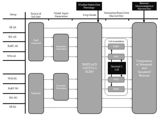
• With regard to the average total biomass of winter wheat at harvest per field: How does the crop model prediction perform when using either analyzed soil texture (in the following: AS) or texture extracted from SoilGrids (in the following: SG) as model input in a standard run (i.e., no ensemble creation, no LAI assimilation), the ensemble mean (i.e., no LAI assimilation), and combined with the assimilation of S2 LAI information based on either of two different approaches (ensemble Kalman filter and weighted mean)?
• Which approach, in combination with AS or SG, reproduces the measured spatial variability of aboveground biomass at harvest within a field better?

2. Materials and Methods

2.1. Experimental Fields and Data Collection

We collected data from fourteen conventionally farmed fields across Germany, France, and the Netherlands (seven fields during the growing season 2016/2017, another seven during the growing season 2017/2018, see Figure A1 in the Appendix A for a map), where winter wheat was grown in the locally practiced crop rotation. Field sizes varied between 7 hectares and 100 hectares. In 2016/2017, one distinct commercially available cultivar was planted on at least two different dates (with field 2 being the only exception with one planting date only) in each location. In 2017/2018, two cultivars were planted per field on the same date (with field 12 being an exception, where seeds from both cultivars were planted on two dates). Plant protecting agents, growth regulators, and fertilizers were applied based on best practice guidelines in accordance with local recommendations. We did not apply any irrigation.

We drew soil samples in 40 to 60 randomly distributed points per field, and analyzed them for texture composition (divided into the particle sizes sand, silt, clay and gravel according to the German classification system [39]) as well as total organic carbon content in the laboratory. German fields were sampled up to a depth of 90 cm in 30 cm intervals, and up to 60 cm on the French and Dutch fields (see

Table 1. Per-field mean values for different particle sizes (gravel, sand, silt, clay) and soil depths for soil samples analyzed in the lab (=AS) and extracted from SoilGrids (=SG) for sampling locations. All values expressed in mass fraction in %.

Field		Gravel AS	Gravel SG	Sand AS	Sand SG	Silt AS	Silt SG	Clay AS	Clay SG
1	0–30	0.02	6.96	4.25	26.46	75.95	58.24	19.8	15.31
	30–60	0.02	6.96	3.48	26.46	75.4	58.24	21.12	15.31
	60–90	0.15	7.67	3.26	25.19	76.01	58.10	20.73	16.71
2	0–30	1.07	4.08	54.46	38.14	29.61	43.28	15.93	18.58
	30–60	0.66	4.28	52.06	39.17	27.69	42.61	20.26	18.22
	60–90	0.47	5.08	56.64	38.17	25.59	43.14	17.77	18.69
3	0–30	1.52	9.12	37.97	27.22	41.57	54.27	20.46	18.52
	30–60	1.32	8.48	34.04	27.25	40.65	54.23	25.31	18.52
	60–90	3.34	9	36.18	25.22	39.79	54.78	24.02	20
4	0–30	0.92	8.46	10	27.39	62.93	49.01	27.06	23.6
	30–60	1.05	8.46	7.96	27.78	55.91	48.76	36.13	23.46
	60–90	1.41	9.94	8.11	26.67	59.06	48.47	32.82	24.86
5	0–30	22.12	12.96	13.64	23.74	38.25	48.64	48.12	27.62
	30–60	21.58	13.28	13.55	24.33	38.21	48.26	48.26	27.4
6	0–30	0.23	9.89	4.75	16.94	72.3	62.18	22.96	20.88
	30–60	0.05	10.29	2.65	17.71	67.15	61.36	30.2	20.93
7	0–30	0.01	4.52	80.93	80.44	10.26	15.19	8.83	4.37
	30–60	0.03	4.45	78.45	80.98	12.7	14.2	8.85	4.82
8	0–30	0.76	7.37	7.06	22.24	69.22	55.96	26.41	21.8
	30–60	0.72	7.37	8.79	21.51	70.97	57.06	25.11	21.43
	60–90	0.54	8.88	13.56	19.29	75.88	57.9	19.69	22.8
9	0–30	0.03	7.41	6.26	20	65.02	58.48	28.72	21.52
	30–60	0.54	8	4.82	20.3	67.7	58.48	27.48	21.23
	60–90	1.89	8.89	4.83	18.89	72.82	59.48	22.35	21.64
10	0–30	0.41	5.83	3.64	26.78	80.7	56.1	15.66	17.12
	30–60	0	5.83	3.33	26.97	79.53	56.31	17.15	16.72
	60–90	0	6.52	2.56	25	79.74	55.72	17.7	19.28
11	0–30	0	6.05	4.63	20	84.32	62.33	11.05	17.67
	30–60	0	6.33	3.02	20	85.07	62	11.91	18
	60–90	0	6.33	2.48	18	76.82	62.29	20.71	19.71
12	0–30	2.34	6.83	12.16	21.15	42.85	52.11	44.99	26.74
	30–60	1.94	7.02	10.93	21.64	48.1	51.89	40.97	26.47
	60–90	4.01	7.62	9.1	18.73	52.17	53.74	38.73	27.53
13	0–30	0.2	6.24	2.8	18.34	82.3	63.95	14.91	17.71
	30–60	0	6.13	2.06	19	81.82	63.37	16.12	17.63
	60–90	0	7.45	1.49	17.55	83.88	64.24	14.64	18.21
14	0–30	0.25	6.19	4.47	17.26	84.2	61.91	11.33	20.84
	30–60	0	6.19	2.9	18.56	83.76	61.05	13.33	20.4
	60–90	0	7.51	1.98	16.86	81.27	61.74	16.75	21.4

for mean values of different soil depths per field). Because of the presence of solid gypsum in deeper layers, some points in field 5 were sampled to a depth of 30 cm only. The minimum distance between two sampling points was 15 m.

Daily weather data were collected from weather stations (Adcon Telemetry, Klosterneuburg, Austria) installed adjacent to the fields (rainfall, minimum and maximum air temperature, solar radiation, and wind speed).

Around maturity, aboveground biomass was sampled at each soil sampling point on an area of 1 m², split into the component grain, stem, and leaves, oven dried at 105 °C until no further weight loss occurred, and weighed subsequently. Average total aboveground biomass yield per field varied between 969 g m⁻² (Field 5, France) and 1959 g m⁻² (Field 3, Germany), the harvest index (i.e., the ratio of grain yield to total aboveground biomass as a measure of reproductive efficiency) varied between 0.41 (Field 2, Germany) and 0.55 (Fields 1 and 7, Germany and Netherlands). Detailed information on the fields investigated in this study can be found in

Table A1. List of study fields and their respective locations. BMY: average total aboveground biomass yield (g m^-2), GY: average grain yield (g m^-2), HI: harvest index, DE: Germany, FR: France, NL: Netherlands.

Country	Growing Season	Field	Location	Cultivar Grown	Planting Date	BMY	GY	HI
DE	2016/2017	1	Central Saxony	Benchmark	2016-10-19	1645	912	0.55
					2016-11-30
DE	2016/2017	2	Southern Northrine-Westphalia	Jonny	2016-10-25	1455	597	0.41
DE	2016/2017	3	Northern Hesse	Julius	2016-10-04	1959	1023	0.52
					2016-10-28
DE	2016/2017	4	Northern Bavaria	RGT Reform	2016-10-05	1737	905	0.54
					2016-10-19
FR	2016/2017	5	Northwestern Charente	Bologna	2016-10-29	969	434	0.44
					2016-11-15
FR	2016/2017	6	Northern Oise	Lyrik	2016-10-03	1579	868	0.54
					2016-10-18
NL	2016/2017	7	Eastern Drenthe	RGT Reform	2016-10-19	1573	876	0.55
					2016-11-03
					2016-11-14
DE	2017/2018	8	Northern Bavaria	RGT Reform	2017-11-03	1451	773	0.53
				JB Asano
DE	2017/2018	9		RGT Reform	2017-11-16	1640	809	0.49
				JB Asano
DE	2017/2018	10	Central Saxony	RGT Reform	2017-09-21	1889	1008	0.53
				JB Asano
DE	2017/2018	11		RGT Reform	2017-10-16	1882	954	0.50
				JB Asano
DE	2017/2018	12	Central Thuringia	JB Asano	2017-09-19, 2017-10-19	1242	527	0.42
				RGT Reform
DE	2017/2018	13	Central Lower Saxony	RGT Reform	2017-11-03	1451	808	0.55
				JB Asano
DE	2017/2018	14		RGT Reform	2017-10-17	1795	889	0.49
				JB Asano

in the Appendix A.

2.2. SoilGrids Soil Information

The SoilGrids REST (representational state transfer) application programming interface was used to request the soil properties bulk density (BLDFIE), clay content (CLYPPT), silt content (SLTPPT), sand content (SNDPPT), content of coarse fragments (>2 mm) (CRFVOL), and soil organic carbon content (ORCDRC) of every exact location where soil samples in each field were taken. SG delivered information for seven standard depths (0 cm, 5 cm, 15 cm, 30 cm, 60 cm, 100 cm, and 200 cm). We calculated the weighted average of the clay and coarse fragments content using numerical integration over the depths 0–30 cm, 30–60 cm, and 60–100 cm (as suggested by [27]) in order to compare those values to the measured ones (see Table 1 for results).

2.3. Leaf Area Index Estimations

The Sentinel Application Platform (SNAP) Sentinel-2 Toolbox Biophysical Processor was used to derive LAI maps for every field (with a pixel resolution of 10 m) based on Sentinel-2 imagery that was atmospherically corrected using the Sen2Cor algorithm [40], with all bands resampled to 10 m resolution (using the Nearest method in SNAP). The Biophysical Processor uses the Sentinel-2 top of canopy reflectance data (coming from the bands 3-8a, 11, and 12) as input into a neural network to calculate LAI for each pixel. The neural network implemented in the biophysical processor was trained using PROSAIL model output—see [35] for a detailed description of the workflow implementation.

LAI values were extracted from each pixel of each image where a soil sampling point was located, using the raster package [41] implemented in R [42], and checked for validity (magnitude of values plus temporal consistency, data not shown). Figure 1 shows the per field acquisition dates of cloud free S2 imagery that were used in this study.

Since we wanted to evaluate how suitable our approaches were as biomass yield predictions tools, we decided to only assimilate LAI observations before the estimated flowering date (i.e., the simulations ran far beyond the assimilation of the last available observation).

Data availability was better in 2018 than in 2017 (see Figure 1). In 2017, every field was covered by at least four images within the period March to June, with a maximum of eight images (field 5). In 2018, every field was covered by at least eleven images within the period March to June, with a maximum of 15 images (field 11).

2.4. Crop Model

We employed the generic LINTUL5 model implemented in the modeling framework SIMPLACE (www.simplace.net, accessed 20 January 2020) to simulate daily leaf area and biomass development in all fields. LINTUL5 is a crop growth simulation model developed for potential water-limited, N-limited, and NPK-limited conditions [43], and has been used widely for crop response assessments [44,45,46].

SIMPLACE (Scientific Impact Assessment and Modelling Platform for Advanced Crop and Ecosystem Management) is a model framework that allows the solution of a modeling problem to be modularized into a number of discrete, replaceable, and interchangeable software units (so-called SimComponents) [47]. The solution used for this study was a combination of the SimComponents LINTUL5, SlimRoots, SlimWater, and STMPsim.

Crop growth in LINTUL5 is a function of intercepted radiation, temperature, and radiation use efficiency (RUE). Daily LAI is calculated as the product of the development stage-dependent specific leaf area (SLA) and the weight of the living green leaves (WLVG).

Soil water balance was simulated using SlimWater, where the daily change in soil water content in a multiple layered soil profile is based on the volumes of crop water uptake, soil evaporation, surface run-off, and seepage below the root zone [48]. Root growth was simulated using the SimComponent SlimRoots, where the daily increase in biomass of seminal and lateral roots depends on the input of assimilated biomass from the shoot (see [47] for more information). Soil hydraulic properties based on the measured texture and texture drawn from SoilGrids (see above) were predicted using the database of hydraulic properties of European soils (HYPRES) [49] pedotransfer functions (PTF) for each soil profile. The functions are based on soil hydraulic data provided by a range of institutions from 12 European countries and are applicable to studies at European scale [49]. Research suggests that the accuracy and reliability of pedotransfer functions may be appropriate for applications from regional to national scale [50].

The layered soil profile consisting of the measured data was extended to 200 cm soil depth, assuming the same in situ texture present as in the 60–90 cm layer.

We assumed no occurrence of disease stress and optimal nutrient supply at all times, as all fields were conventionally managed in accordance with local recommendations. Thus, water stress was the only growth-limiting factor considered in the model. In our SIMPLACE <LINTUL5,SLIM> solution, water stress was imposed on biomass production if the calculated actual transpiration of the crop dropped below the calculated potential transpiration because of the insufficient levels of transpirable soil water in the root layer. Evapotranspiration was estimated based on the Applied Penman approach [43].

SIMPLACE <LINTUL5, SLIM> ran in daily time steps. Daily phenology data were provided by a xarvio^TM in-house developed, commercial growth stage model that estimated cultivar-specific BBCH stages of winter wheat based on the accumulated thermal temperature, vernalization, and photoperiod. The growth stage model was developed for better estimation of fungicide application timing, and has been validated with roughly 30,000 records in Germany. The BBCH stages were transformed into the LINTUL-internal development stages (DVS) based on a lookup-table, and linked to all SimComponents that required DVS information. For all winter wheat-specific variables beyond phenology, we used the generic values (i.e., no calibration of cultivar specifics). Daily meteorological data needed in the simulation model was taken from the data provided by the weather stations.

2.5. Data Assimilation

We implemented two approaches to assimilate LAI values into SIMPLACE <LINTUL5, SLIM>: The ensemble Kalman filter (EnKF) and the weighted mean (WM) approach. EnKF has gained popularity in the scientific community because of its simple conceptual formulation and ease of implementation, plus its low computational requirements [51]. It combines an ensemble forecast and the Kalman filter to calculate the prediction error covariance using the Monte Carlo method [19]. State variables are updated sequentially, taking the uncertainties of the simulation results and observations into account [52]. We refer to other publications for detailed information about EnKF [3,51]. The integration into SIMPLACE<LINTUL5, SLIM> was done in R [42] using the SIMPLACE R wrapper [53], relying on the EnKF implementation provided by Stefan Gelissen (http://blogs2.datall-analyse.nl/2016/06/08/rcode_ensemble_kalman_filter/, accessed 9 November 2019). The workflow constituted as follows: First, the ensemble members were randomly generated based on the chosen initial values and variance. Second, model runs using the sets of variables as input were invoked. Simulations run until the first S2 LAI observation became available. This interrupted each model run, EnKF updated the LAI value accordingly, and the runs were re-invoked until the next observation became available.

The WM approach relies on a model ensemble that runs from simulation start to simulation end without compromising the consistency and integrity of the state variables in the ensemble runs. It is based on the attribution of weights to the model ensemble members depending on their proximity between simulation and observation at the first date of LAI observation. These weights are then updated at the subsequent observation dates and used in the calculation of the ensemble mean at each model time step. The efficiency is comparable to those of updating methods. Methodology and test results are documented in detail in our publication (currently under review) [54].

Both approaches (EnKF and WM) relied on the generation of a model ensemble. We chose a set consisting of soil and crop components (SCC) that comprised the combination of three variables that scaled (1) the soil water content at simulation start (SoilWaterInit), (2) the maximal rooting depth that could be reached by the plants (MaximalRootDepth), and (3) a scaling factor for the DVS-dependent specific leaf area (ScaleFactorSLA). By perturbing the first two variables at initialization, the model induced water stress (by modification of the transpiration reduction factor TRANRF) at varying points in time during the growing season, thereby expanding the range of LAI values at any given point in time in the ensemble. We did not alter both parameters after initialization for reasons of model consistency. ScaleFactorSLA scaled all predefined DVS-dependent SLA values uniformly and showed high impact on LAI dynamics and biomass accumulation in the model, and was included as to cover influences of possible hidden factors (such as nutrient stress).

The initial soil water content SoilWaterInit in soil layer k was calculated as

$$SoilWaterIni{t}_k=ScalingFactor\ast VolumetricWaterContent33to{1500}_k+VolumetricWaterContent{1500}_k,$$

(1)

where VolumetricWaterContent33to1500 describes the volumetric soil water content between field capacity and wilting point (i.e., plant available water), and VolumetricWaterContent1500 the volumetric soil water content at permanent wilting point. Both values were returned by the pedotransfer function (see above), based on the measured soil texture.

We chose a uniform parameter distribution for the WM approach, with defined minimum and maximum values (SoilWaterInit 0.3-1, MaximalRootDepth 0.5-2, ScalingFactorSLA 0.75-1.25). EnKF creates a model ensemble using a randomly generated Gaussian distribution of the variables (mean values for the distribution: SoilWaterInit 0.65, MaximalRootDepth 1.25, ScalingFactorSLA 1.25).

To achieve a maximum effect of the varying initial soil conditions on crop development, simulation start was set to the day preceding sowing. The LAI error was assumed 0.3.

2.6. Model Run and Evaluation

We decided to compare the two SG and AS derived soil texture fractions “clay” and “gravel,” as differences generally impact the soil moisture dynamics in the simulated soil profile. We calculated the Pearson correlation coefficient (r), the root mean squared error (RMSE), and the bias for each field and soil fraction, comparing each soil layer (0–30 cm, 30–60 cm, and 60–90 (-100 for SG) cm) accordingly. Additionally, we also included the absolute average available water content (AWC, 0–90 cm) calculated by the HYPRES pedotransfer function.

The assessment of the crop model biomass predictions with regard to AS, SG, and the combination of the two different assimilation approaches was based on the comparison of measured and simulated total aboveground biomass at harvest day. For this, SIMPLACE<LINTUL5, SLIM> ran in daily time steps for every sampling point in every field that was part of this study, once using AS and once using SG as input. All available Sentinel-2 LAI estimations for every sampling point were assimilated into the model using the approaches EnKF and WM in combination with the SCC ensemble generation set. Other studies have shown that crop growth simulation model predictions improve if LAI, observed over several growth stages, is assimilated [12,14].

To evaluate the potential benefit of data assimilation, we also included the ensemble mean (EM, i.e., no data assimilation, run with measured and SoilGrids extracted soil texture data using the same ensemble generation method as the WM approach) and the model’s standard runs (SR) (i.e., no data assimilation, no ensemble creation, run with single point input from AS and SG using the standard configuration) in the analysis. A workflow for all setups is provided in Figure 2.

We calculated the three metric RMSE, mean absolute percentage error (MAPE), and the bias. RMSE indicated the magnitude of error in the unit of measurement with symmetry provided; MAPE showed the average absolute percent difference between measured and predicted values, the bias computed the amount by which the measured values were greater or smaller than the predicted ones. We assumed that the crop model simulated spatial heterogeneity of biomass yield well if the value of each metric was close to zero.

3. Results

3.1. Comparison of Measured Soil Texture Data and Texture Data from SoilGrids

The results of the comparison of measured soil texture data and SoilGrids texture data per field are presented in

Table 2. Per-field results of comparison of measured soil texture data and texture data extracted from SoilGrids as well as plant-available water content derived from the HYPRES pedotransfer functions. R: Pearson correlation coefficient, RMSE: root mean squared error, AS: analyzed soil texture, SG: SoilGrids-extracted soil texture, AWC: available water content. RMSE and bias in mass fraction in %. All values show mean values per field. Positive bias values indicate overestimation by SoilGrids.

	Clay Content			Gravel Content			Plant-Available Water Content
Field	R	RMSE	Bias	R	RMSE	Bias	R	RMSE	Bias	AWC AS (%)	AWC SG (%)
1	−0.05	5.14	−2.27	−0.01	9.58	9.39	−0.21	0.03	−0.03	0.17	0.14
2	0.49	5.27	0.81	−0.22	5.16	4.95	−0.22	0.01	−0.01	0.124	0.133
3	0.45	5.67	−2.59	0.16	12.05	10.42	0.53	0.01	0	0.133	0.13
4	0.24	11.65	−5.93	−0.02	10.70	10.37	−0.12	0.02	−0.01	0.135	0.122
5	0.00	17.61	−16.25	−0.05	8.91	−7.28	0.22	0.05	0.05	0.184	0.112
6	0.67	6.17	−4.87	0.05	9.94	9.92	0.27	0.02	−0.02	0.15	0.134
7	−0.17	5.13	−4.07	0.03	4.30	4.28	0.09	0.04	0.04	0.106	0.145
8	−0.60	4.75	0.67	−0.21	10.26	10.04	0.34	0.03	−0.03	0.157	0.13
9	−0.53	6.08	−2.38	0.55	10.13	9.99	−0.11	0.02	−0.02	0.152	0.133
10	0.31	4.44	3.77	−0.53	8.39	8.18	0.27	0.04	−0.04	0.177	0.138
11	0.84	7.40	6.66	NA	9.83	9.52	0.52	0.04	−0.04	0.184	0.142
12	−0.04	14.16	−13.20	0.27	7.09	6.64	0.71	0.02	0.02	0.107	0.123
13	0.33	4.01	3.80	−0.63	8.38	8.27	0.60	0.04	−0.04	0.183	0.142
14	0.59	8.14	7.89	−0.53	7.95	7.89	−0.01	0.05	−0.05	0.186	0.135

. A strong positive agreement (r > 0.8) could only be seen for the clay content in field 11, while other fields showed weak to no agreement at all (r~0) (e.g., fields 1, 5, 12), and some even showed negative agreements (r < 0, e.g., field 8). RMSE values ranged between 4.01% (field 13) and 17.61% (field 5) mass fraction for clay content, and between 4.3% (field 7) and 12.05% (field 3) mass fraction for gravel content. For the most part, SoilGrids data underestimated the clay content and overestimated the gravel content in the field (positive bias values indicate overestimation by the SoilGrids data). Altogether, it was obvious that the SoilGrids data did not predict the measured soil texture well in any of the fields.

The analysis of the PTF-derived plant-available water content (AWC, i.e., volumetric soil water content at field capacity to wilting point pF2.5) showed no strong relationship in any of the fields; some fields show moderately strong relationships (e.g., fields 3, 11, 12), others no relationship (fields 7, 14), some more even negative relationships (fields 1, 2, 9). The average calculated AWC is lower in the SG data than in the AS data in most fields (except fields 2, 7, and 12).

3.2. Comparison of Simulated vs. Measured Aboveground Biomass

Figure 3 shows the mean RMSE and standard deviation of total aboveground biomass across all fields for the tested approaches. The highest RMSE was produced by SR AS (532.39 g m⁻²) with a standard deviation of 158.12 g m⁻², the lowest by EM SG (246.63 g m⁻²) with a standard deviation of 123.84 g m⁻². However, it is noticeable that all approaches but the standard runs show, on average, similar performances with a mean value of about 250 g m⁻².

The lowest MAPE, averaged across all fields, was produced by EnKF AS (0.14 with a standard deviation of 0.06) and WM AS (0.14 with a standard deviation of 0.07), the highest by SR AS (0.35 with a standard deviation of 0.14) and SR SG (0.25 with a standard deviation of 0.23). The SoilGrids-based approaches showed higher standard deviations than the analyzed soil texture-based approaches, with similar mean values, however (Figure 4).

On average across all fields, the greatest bias was produced by SR AS (484.52 g m⁻² with a standard deviation of 168.51 g m⁻²), the lowest by EM SG (15.37 g m⁻² with a standard deviation of 229.77 g m⁻²) and EnKF SG (−32.66 g m⁻² with a standard deviation of 269.24 g m⁻²) (Figure 5). Those approaches using SG as model input tended to produce a lower bias with a higher standard deviation in comparison with those approaches using measured soil texture as model input (which produced higher bias values with lower standard deviations).

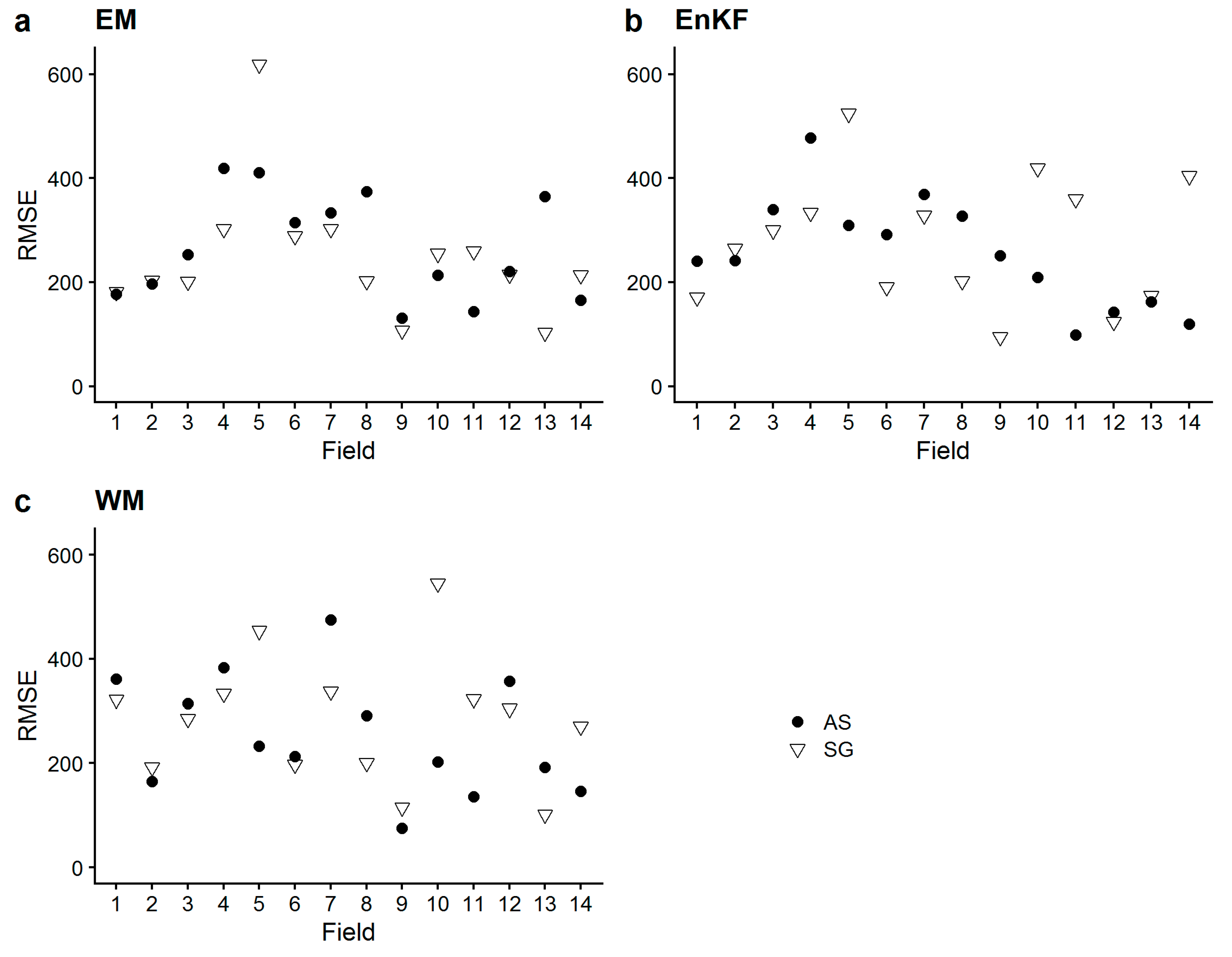
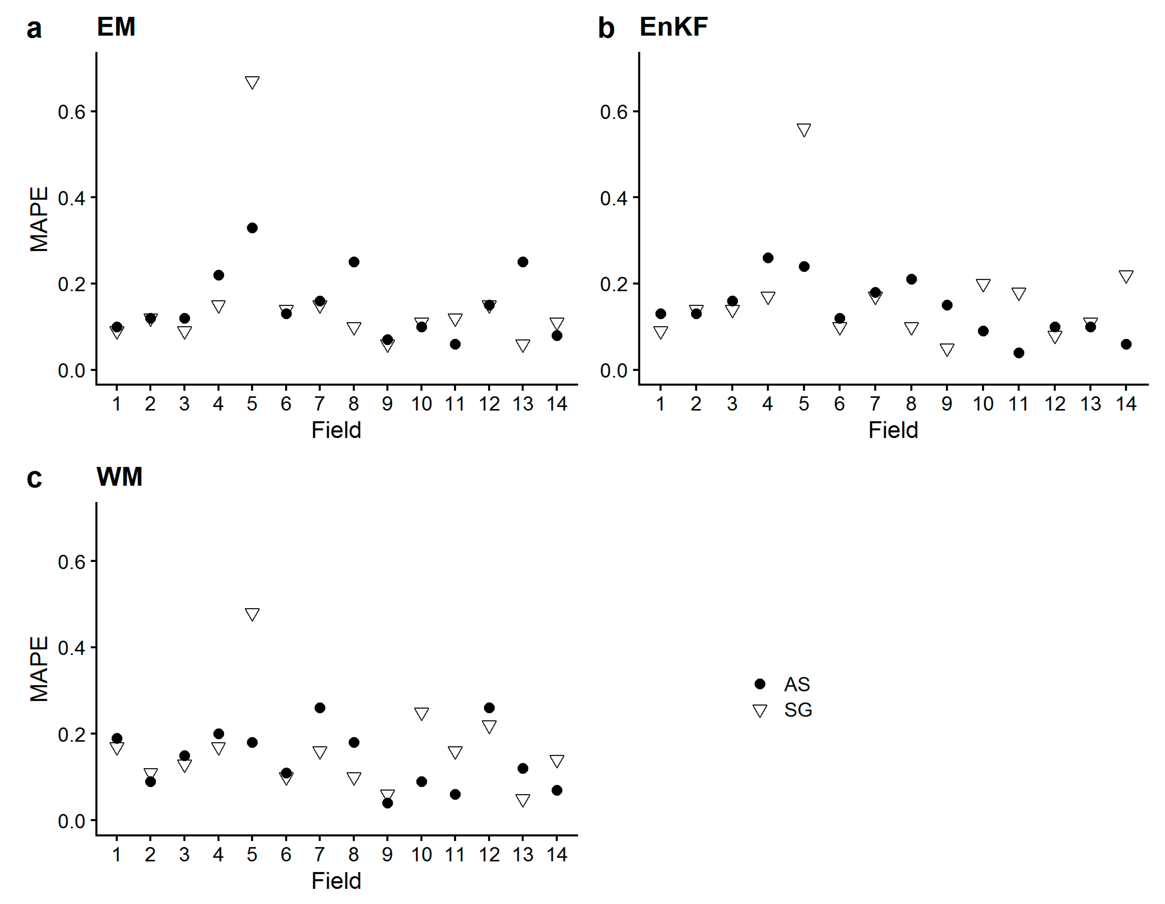
3.3. Assessment of Reproduction of Sub-Field Variability

Our assessment of the sub-field reproduction of our approaches is based on the analysis of the metrics RMSE, MAPE, and bias, assuming that values closer to 0 show a greater agreement with field-measured biomass at harvest day. We decided to exclude the approaches SR AS and SR SG from further analysis because of their inferior average performances (see previous section). Figure 6, Figure 7 and Figure 8 show the per-field results of RMSE, MAPE, and bias for EM (a), EnKF (b), and WM (c) approaches, either using analyzed soil or SoilGrids-derived texture as model input.

It is obvious in all three figures that performances of both AS and SG were highly variable between fields and between approaches (EM, EnKF, and WM), as well as per field. No single approach stood out, and neither AS or SG showed a systematically better performance across all fields.

4. Discussion

4.1. Results of the SoilGrids vs. Measured Soil Texture Comparison

With regard to research question 1, the analysis of the SoilGrids vs. analyzed soil texture showed that (1) SG did not predict the field-measured soil texture well (clay content was largely underestimated and gravel content was largely overestimated) across the soil profiles down to 90 cm soil depth, and (2) the plant-available soil water volumetric content derived from the PTFs was substantially lower for SG in most of the fields than for AS. A number of studies have been reported on the limitations of the SoilGrids system [55,56,57], and the authors themselves advise on their homepage to, if national or local scales are targeted, compare the predictions with soil maps derived from national and local soil databases, since they are usually based on more detailed input soil information and therefore exhibit greater accuracy (www.soilgrids.org, accessed 19 November 2019). Combining local and global predictions could be a promising possibility, as well as the creation of SoilGrids at higher spatial resolution based on state-of-the-art remote sensing products that are relevant for soil mapping [27]. Currently, SoilGrids show the highest accuracy and resolution among the soil datasets covering the world [58], and was therefore our information source of choice.

4.2. Results of the Crop Modeling Excersises

The SoilGrids system generally provides worldwide soil property predictions at 250 m resolution [27]. Soil information for each field was therefore provided by few grid cells only, and thus identical estimated soil texture information was assigned to all sampling points located inside one corresponding grid cell. Spatial heterogeneity in the biomass predictions of the SG-based assimilation approaches could therefore only be induced by a) the differences in soil texture information if the field stretched over more than one grid cell (for SR), and/or b) the assimilation of S2-derived LAI information (for EM, EnKF, and WM) that was extracted from 10 m resolution pixels, because all other input variables were identical in the model for each point in the field (weather data, crop specific variables). Contrary to this, spatial heterogeneity in the biomass predictions of the AS-based approaches was a mixed effect of individual soil properties (for SR and EM) and assimilated S2-derived LAI (for EnKF and WM).

Given these limitations, our expectations with regards to the research questions 2 and 3 therefore were that 1) the performance of the crop model biomass predictions with SG-based approaches will be worse because of inaccurate soil texture information, leading to inaccurate modeling of soil moisture and root growth dynamics that ultimately affect the biomass production; 2) those approaches that rely on the assimilation of S2-derived LAI into the crop model will perform better in predicting biomass yield than those approaches without assimilation, because potential model inaccuracies will be corrected for; and 3) spatial heterogeneity of biomass yield in the SG-based approaches will not be as accurately reproduced as in the AS-based approaches because processes that influence biomass production after flowering are not accurately accounted for because of inaccurate soil information.

The analysis of the results showed that:

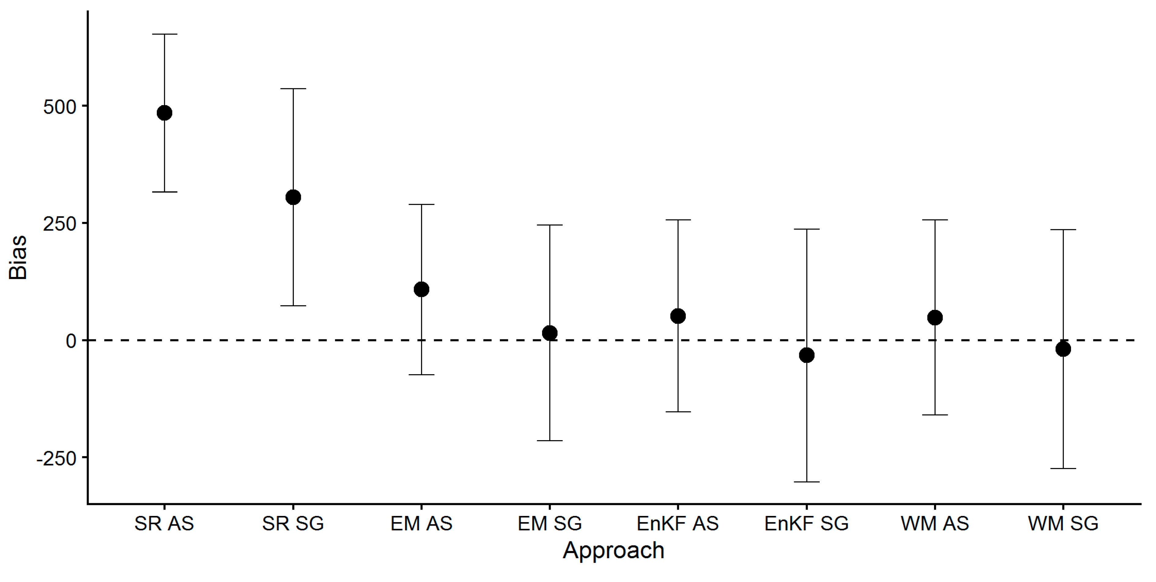
• Mean values of the calculated metrics (RMSE, MAPE, Bias) across all fields did not substantially differ between ensemble-based SG and AS approaches (i.e., EM, EnKF, WM), but standard deviations were greater for SG-based approaches. The model’s standard runs (SR, i.e., no assimilation, no ensemble generation), performed worse, and biomass yield was largely overestimated as indicated by the positive bias.These findings show that the average biomass prediction performance based on SG soil information was not inferior to AS soil information prediction performance, but came with a greater prediction uncertainty.
• The simulated sub-field heterogeneity of biomass at harvest did not accurately match the measured one in any of the sites, as no approach showed a congruent performance for any of the metrics. AS-based approaches did not outperform SG-based approaches concerning the reproduction of heterogeneity. The performance of the assimilation approaches were largely site-specific, as we saw the approaches performing differently in the different sites, with no clear approach standing out. To our surprise, EM did not perform substantially worse.

Water stress was the only stress (i.e., biomass growth inhibiting) factor that we considered in our SIMPLACE <LINTUL5,SLIM> model solution. Differences between AS and SG approaches with the same setup could therefore only be caused by differences in soil water dynamics and/or root growth simulations that cause diverging levels of water stress. The SLIM components of the model failed to simulate soil-related processes adequately, as the setups without data assimilation using field-measured soil texture (SR AS and EM AS) overestimated, on average, biomass yield to a larger extent than the SR SG and EM AS using SoilGrids-derived soil texture (as indicated by the bias). The assimilation of LAI information, however, alleviated this effect (as the mean bias of EnKF AS and EnKF SG as well as WM AS and WM SG are similar).

The methods of simulating soil water dynamics vary between crop simulation models, with different approaches for soil water movement (e.g., tipping bucket or Richard’s approach), different degrees of resolution (e.g., number of soil layers) and weather variables (e.g., approaches for the calculation of evapotranspiration) [59]. While there is probably no single approach that works best in all cases, we encourage a comparative study to investigate the effects of different soil water dynamic simulation approaches on the results of our methodology.

4.3. Limitations of Input Data

The pedotransfer functions developed from the HYPRS database allow for the assignment of hydraulic properties to soils in Europe that show similar textural compositions. Thus, those functions should not be used to derive hydraulic properties outside Europe, as the lack of data suggests a risky extrapolation [49]. This means that, currently, our model solution is limited to an application in Europe only. Scientists in other parts of the world are therefore encouraged to rely only on predictions made for soils that were inside the range of soils used to derive the pedotransfer functions.

The aboveground biomass measurements at harvest comprised one measurement per sampling point only (i.e., no repetitive measurements). The values could therefore be prone to measurement errors. This uncertainty should be considered when interpreting the results based on simulated vs. observed results. Furthermore, differences in phenology were the only cultivar-specific properties we considered in this study. The model was not calibrated for other variables (e.g., SLA, RUE) that could have influenced the results positively.

4.4. Sentinel-2 LAI Estimations

In this study, LAI estimations were obtained directly through the SNAP Sentinel-2 Toolbox Biophysical Processor. The algorithm is based on a set of strong assumptions associated with the underlying PROSAIL radiative transfer model (regarding leaf optical properties, canopy structure and background reflectance, see [35]). Violations of those assumptions may generally lead to differences with ground truth measurements, but could be corrected for with a custom correction accounting for the specificities of the given type of canopy [35]. Given this, we decided to forgo a validation exercise.

We are currently not aware of any other tool that provides automated LAI estimates at Sentinel-2 or greater spatial resolution (i.e., at resolutions that are of interest for precision farming applications). Arguably, this approach offers great opportunities for crop modelers, as LAI estimations can be derived without much effort. We encourage the implementation for other multispectral satellites (e.g., Landsat-8, PlanetScope).

Contrary to other studies, we cannot confirm that assimilating S2-derived LAI into a crop model improves the general prediction accuracy. Our results suggested that relying on an EM approach might lead to satisfactory results, comparable to those that were produced with the help of LAI assimilation. Furthermore, despite its shown inaccuracy at small scale, SoilGrids data proved not to provide information that lead to totally diverging results from those that used analyzed soil information as model input. However, the reader should keep in mind that, among all sites, none of the approaches showed an outstanding performance. This means that, if one approach works fine for one site, it might not perform well for another site.

Ref [13] assimilated Sentinel-2 derived LAI into the EPIC (Environmental Policy Integrated Climate) model to estimate winter wheat grain yield on Austrian experimental fields under four fertilization management strategies over the course of two growing seasons, using field-measured soil characteristics as model input. They found that assimilation via recalibration of parameters defining the LAI curve improved the model’s performance notably during the first year (RMSE 317 kg ha⁻¹, RRMSE 6% compared to RMSE 572 kg ha⁻¹, RRMSE 11% without assimilation), but only slightly during the second year (RMSE 1961 kg ha⁻¹, RRMSE 55% compared to RMSE 2019 kg ha⁻¹, no RRMSE reported), with a strong underestimation of the observed yield. They attribute this underestimation to (a) rainfall possibly not representative of the site as weather data from a station 30 km away was used, (b) non-representative model default parameters for the specific year, and (c) erroneously modelled water stress conditions. [7] assimilated Sentinel-2-derived LAI into the WOFOST (World Food Studies) model for winter wheat grain yield prediction at field scale in the North China Plain, with soil information extracted from the 1:1,000,000 China Soil Database used as model input. The authors found that the assimilation, relying on EnKF, decreased the RMSE by 69 kg ha⁻¹ to 404 kg ha⁻¹ (MRE 4.32%). They furthermore found that the joint assimilation of LAI and soil moisture estimations showed superior performance in estimating crop yield, but concluded that soil moisture assimilation may not be necessary under very wet conditions [7]. [2] used LAI data derived from Landsat-8, Landsat-7, and Sentinel-2A images to correct the WARM rice model via automatic recalibration of crop parameters at sub-field resolution for 40 paddy fields in northern Italy. They found that assimilating LAI increased the overall accuracy (MAE 0.66 t ha⁻¹, RRMSE 13.8%), and that sub-field yield variability, in most cases, was well reproduced. Occurring inconsistencies were attributed to possibly erroneous LAI data or factors that were not considered by the model, such as effects of previous cover crop or extreme weather events [2].

5. Conclusions

The objectives of this study were to: (1) Compare detailed soil texture measurements from 14 fields across France, Germany, and the Netherlands to soil texture information drawn from SoilGrids for the exact same locations; (2) investigate the performance of the crop model solution SIMPLACE<LINTUL5, SLIM> in those locations when using either analyzed or SoilGrids texture as model input in a range of setups in- and excluding the assimilation of Sentinel-2 estimated LAI with regard to average total biomass of winter wheat at harvest; and (3) investigate which approach, in combination with the provided soil texture information, reproduced spatial variability of aboveground biomass at harvest within the fields better.

Despite the inaccurate soil texture information provided by SoilGrids for the locations of the sampling points in the fourteen fields (clay content was largely underestimated, and gravel content was largely overestimated), the mean results of the performance of the SG-based model runs did not differ substantially from the AS-based model runs, for all ensemble-based approaches. We therefore reasoned not to advise against using this source of soil information as crop model input; the user should, however, be aware of greater uncertainty in the prediction (we found a higher standard error with similar mean values for the SG-based approaches). We furthermore concluded that, contrary to other studies, the assimilation of S2-derived LAI (using EnKF and WM) into the crop model did not improve the general prediction accuracy (average over all field), as the results of the EM runs (i.e., without assimilation) were similar. Sub-field variability of aboveground biomass at harvest was not reproduced accurately in any of the fields, because of inaccurate simulation of water stress that influences biomass accumulation dynamic in the crop model.

Based on the findings and discussed limitations of this study, we encourage future researchers to (1) evaluate the performance of other crop models that rely on different approaches to simulate soil moisture dynamics (e.g., Richards approach) and evapotranspiration (Penman–Monteith, Priestley–Taylor, Turc, …) when using either measured or SoilGrids-estimated soil texture as input in combination with assimilated LAI to see if water stress is simulated more accurately; (2) test our approaches in other cropping sites around the globe and/or for other crops to investigate if our findings can be confirmed in different environmental conditions and a variable availability of cloud free satellite imagery; (3) use different sets of remote sensing data to see the effect of variable spatial resolutions; and (4) include further stresses that might alter biomass production (e.g., nutrient stress, heat stress).

References

1. Verrelst, J.; Camps-Valls, G.; Muñoz-Marí, J.; Rivera, J.P.; Veroustraete, F.; Clevers, J.G.P.W.; Moreno, J. Optical remote sensing and the retrieval of terrestrial vegetation bio-geophysical properties—A review. ISPRS J. Photogramm. Remote Sens. 2015, 108, 273–290. [Google Scholar] [CrossRef]
2. Gilardelli, C.; Stella, T.; Confalonieri, R.; Ranghetti, L.; Campos-Taberner, M.; García-Haro, F.J.; Boschetti, M. Downscaling rice yield simulation at sub-field scale using remotely sensed LAI data. Eur. J. Agron. 2019, 103, 108–116. [Google Scholar] [CrossRef]
3. Wallach, D.; Makowski, D.; Jones, J.W.; Brun, F. Chapter 8—Data Assimilation for Dynamic Models. In Working with Dynamic Crop Models, 2nd ed.; Wallach, D., Makowski, D., Jones, J.W., Brun, F., Eds.; Academic Press: San Diego, CA, USA, 2014; pp. 311–343. ISBN 978-0-12-397008-4. [Google Scholar]
4. Chen, Y.; Zhang, Z.; Tao, F. Improving regional winter wheat yield estimation through assimilation of phenology and leaf area index from remote sensing data. Eur. J. Agron. 2018, 101, 163–173. [Google Scholar] [CrossRef]
5. De Wit, A.J.W.; van Diepen, C.A. Crop model data assimilation with the Ensemble Kalman filter for improving regional crop yield forecasts. Agric. For. Meteorol. 2007, 146, 38–56. [Google Scholar] [CrossRef]
6. Hu, S.; Shi, L.; Huang, K.; Zha, Y.; Hu, X.; Ye, H.; Yang, Q. Improvement of sugarcane crop simulation by SWAP-WOFOST model via data assimilation. Field Crop Res. 2019, 232, 49–61. [Google Scholar] [CrossRef]
7. Pan, H.; Chen, Z.; de Wit, A.; Ren, J. Joint Assimilation of Leaf Area Index and Soil Moisture from Sentinel-1 and Sentinel-2 Data into the WOFOST Model for Winter Wheat Yield Estimation. Sensors 2019, 19, 3161. [Google Scholar] [CrossRef] [PubMed] [Green Version]
8. Xie, Y.; Wang, P.; Sun, H.; Zhang, S.; Li, L. Assimilation of Leaf Area Index and Surface Soil Moisture With the CERES-Wheat Model for Winter Wheat Yield Estimation Using a Particle Filter Algorithm. IEEE J. Sel. Top. Appl. Earth Obs. Remote Sens. 2017, 10, 1303–1316. [Google Scholar] [CrossRef]
9. Silvestro, P.C.; Pignatti, S.; Pascucci, S.; Yang, H.; Li, Z.; Yang, G.; Huang, W.; Casa, R. Estimating Wheat Yield in China at the Field and District Scale from the Assimilation of Satellite Data into the Aquacrop and Simple Algorithm for Yield (SAFY) Models. Remote Sens. 2017, 9, 509. [Google Scholar] [CrossRef] [Green Version]
10. Huang, J.; Tian, L.; Liang, S.; Ma, H.; Becker-Reshef, I.; Huang, Y.; Su, W.; Zhang, X.; Zhu, D.; Wu, W. Improving winter wheat yield estimation by assimilation of the leaf area index from Landsat TM and MODIS data into the WOFOST model. Agric. For. Meteorol. 2015, 204, 106–121. [Google Scholar] [CrossRef] [Green Version]
11. Ines, A.V.M.; Das, N.N.; Hansen, J.W.; Njoku, E.G. Assimilation of remotely sensed soil moisture and vegetation with a crop simulation model for maize yield prediction. Remote Sens. Environ. 2013, 138, 149–164. [Google Scholar] [CrossRef] [Green Version]
12. Li, H.; Chen, Z.; Liu, G.; Jiang, Z.; Huang, C. Improving Winter Wheat Yield Estimation from the CERES-Wheat Model to Assimilate Leaf Area Index with Different Assimilation Methods and Spatio-Temporal Scales. Remote Sens. 2017, 9, 190. [Google Scholar] [CrossRef] [Green Version]
13. Novelli, F.; Spiegel, H.; Sandén, T.; Vuolo, F. Assimilation of Sentinel-2 Leaf Area Index Data into a Physically-Based Crop Growth Model for Yield Estimation. Agronomy 2019, 9, 255. [Google Scholar] [CrossRef] [Green Version]
14. Xie, Y.; Wang, P.; Bai, X.; Khan, J.; Zhang, S.; Li, L.; Wang, L. Assimilation of the leaf area index and vegetation temperature condition index for winter wheat yield estimation using Landsat imagery and the CERES-Wheat model. Agric. For. Meteorol. 2017, 246, 194–206. [Google Scholar] [CrossRef]
15. Zhao, Y.; Chen, S.; Shen, S. Assimilating remote sensing information with crop model using Ensemble Kalman Filter for improving LAI monitoring and yield estimation. Ecol. Model. 2013, 270, 30–42. [Google Scholar] [CrossRef]
16. Jonckheere, I.; Fleck, S.; Nackaerts, K.; Muys, B.; Coppin, P.; Weiss, M.; Baret, F. Review of methods for in situ leaf area index determination: Part, I. Theories, sensors and hemispherical photography. Agric. For. Meteorol. 2004, 121, 19–35. [Google Scholar] [CrossRef]
17. Dorigo, W.A.; Zurita-Milla, R.; de Wit, A.J.W.; Brazile, J.; Singh, R.; Schaepman, M.E. A review on reflective remote sensing and data assimilation techniques for enhanced agroecosystem modeling. Int. J. Appl. Earth Obs. Geoinf. 2007, 9, 165–193. [Google Scholar] [CrossRef]
18. Huang, J.; Gómez-Dans, J.L.; Huang, H.; Ma, H.; Wu, Q.; Lewis, P.E.; Liang, S.; Chen, Z.; Xue, J.-H.; Wu, Y.; et al. Assimilation of remote sensing into crop growth models: Current status and perspectives. Agric. For. Meteorol. 2019, 276–277, 107609. [Google Scholar] [CrossRef]
19. Jin, X.; Kumar, L.; Li, Z.; Feng, H.; Xu, X.; Yang, G.; Wang, J. A review of data assimilation of remote sensing and crop models. Eur. J. Agron. 2018, 92, 141–152. [Google Scholar] [CrossRef]
20. Jiang, Z.; Chen, Z.; Chen, J.; Liu, J.; Ren, J.; Li, Z.; Sun, L.; Li, H. Application of Crop Model Data Assimilation With a Particle Filter for Estimating Regional Winter Wheat Yields. IEEE J. Sel. Top. Appl. Earth Obs. Remote Sens. 2014, 7, 4422–4431. [Google Scholar] [CrossRef]
21. Jiang, Z.; Chen, Z.; Chen, J.; Ren, J.; Li, Z.; Sun, L. The Estimation of Regional Crop Yield Using Ensemble-Based Four-Dimensional Variational Data Assimilation. Remote Sens. 2014, 6, 2664–2681. [Google Scholar] [CrossRef] [Green Version]
22. Cheng, Z.; Meng, J.; Shang, J.; Liu, J.; Qiao, Y.; Qian, B.; Jing, Q.; Dong, T. Improving Soil Available Nutrient Estimation by Integrating Modified WOFOST Model and Time-Series Earth Observations. IEEE Trans. Geosci. Remote Sens. 2018, 2896–2908. [Google Scholar] [CrossRef]
23. Li, X.; Du, H.; Mao, F.; Zhou, G.; Chen, L.; Xing, L.; Fan, W.; Xu, X.; Liu, Y.; Cui, L.; et al. Estimating bamboo forest aboveground biomass using EnKF-assimilated MODIS LAI spatiotemporal data and machine learning algorithms. Agric. For. Meteorol. 2018, 256–257, 445–457. [Google Scholar] [CrossRef]
24. Zhuo, W.; Huang, J.; Li, L.; Zhang, X.; Ma, H.; Gao, X.; Huang, H.; Xu, B.; Xiao, X. Assimilating Soil Moisture Retrieved from Sentinel-1 and Sentinel-2 Data into WOFOST Model to Improve Winter Wheat Yield Estimation. Remote Sens. 2019, 11, 1618. [Google Scholar] [CrossRef] [Green Version]
25. Huang, J.; Sedano, F.; Huang, Y.; Ma, H.; Li, X.; Liang, S.; Tian, L.; Zhang, X.; Fan, J.; Wu, W. Assimilating a synthetic Kalman filter leaf area index series into the WOFOST model to improve regional winter wheat yield estimation. Agric. For. Meteorol. 2016, 216, 188–202. [Google Scholar] [CrossRef]
26. Tewes, A.; Hoffmann, H.; Schäfer, F.; Kerkhoff, C.; Krauss, G.; Gaiser, T. Assimilation of Leaf Area Index Measurements Into A Crop Model Framework: Performance Comparison of Two Assimilation Approaches. In Proceedings of the 12th European Conference on Precision Agriculture, SupAgro Montpellier, Montpellier, France, 8–11 July 2019; pp. 182–183, ISBN 978-2-900792-49-0. [Google Scholar]
27. Hengl, T.; de Jesus, J.M.; Heuvelink, G.B.M.; Gonzalez, M.R.; Kilibarda, M.; Blagotić, A.; Shangguan, W.; Wright, M.N.; Geng, X.; Bauer-Marschallinger, B.; et al. SoilGrids250m: Global gridded soil information based on machine learning. PLoS ONE 2017, 12, e0169748. [Google Scholar] [CrossRef] [Green Version]
28. Pätzold, S.; Mertens, F.M.; Bornemann, L.; Koleczek, B.; Franke, J.; Feilhauer, H.; Welp, G. Soil heterogeneity at the field scale: A challenge for precision crop protection. Precis. Agric. 2008, 9, 367–390. [Google Scholar] [CrossRef]
29. Clevers, J.G.P.W.; Kooistra, L.; Van den Brande, M.M.M. Using Sentinel-2 Data for Retrieving LAI and Leaf and Canopy Chlorophyll Content of a Potato Crop. Remote Sens. 2017, 9, 405. [Google Scholar] [CrossRef] [Green Version]
30. Pasqualotto, N.; Delegido, J.; Van Wittenberghe, S.; Rinaldi, M.; Moreno, J. Multi-Crop Green LAI Estimation with a New Simple Sentinel-2 LAI Index (SeLI). Sensors 2019, 19, 904. [Google Scholar] [CrossRef] [Green Version]
31. Xie, Q.; Dash, J.; Huete, A.; Jiang, A.; Yin, G.; Ding, Y.; Peng, D.; Hall, C.C.; Brown, L.; Shi, Y.; et al. Retrieval of crop biophysical parameters from Sentinel-2 remote sensing imagery. Int. J. Appl. Earth Obs. Geoinformation 2019, 80, 187–195. [Google Scholar] [CrossRef]
32. Toscano, P.; Castrignanò, A.; Di Gennaro, S.F.; Vonella, A.V.; Ventrella, D.; Matese, A. A Precision Agriculture Approach for Durum Wheat Yield Assessment Using Remote Sensing Data and Yield Mapping. Agronomy 2019, 9, 437. [Google Scholar] [CrossRef] [Green Version]
33. Vizzari, M.; Santaga, F.; Benincasa, P. Sentinel 2-Based Nitrogen VRT Fertilization in Wheat: Comparison between Traditional and Simple Precision Practices. Agronomy 2019, 9, 278. [Google Scholar] [CrossRef] [Green Version]
34. Pause, M.; Raasch, F.; Marrs, C.; Csaplovics, E. Monitoring Glyphosate-Based Herbicide Treatment Using Sentinel-2 Time Series—A Proof-of-Principle. Remote Sens. 2019, 11, 2541. [Google Scholar] [CrossRef] [Green Version]
35. Weiss, M.; Baret, F. S2ToolBox Level 2 Products: LAI, FAPAR, FCOVER. Sentinel-2 Algorithm Theoretical Based Document. 2016. Available online: https://step.esa.int/docs/extra/ATBD_S2ToolBox_L2B_V1.1.pdf (accessed on 5 March 2020).
36. Pasqualotto, N.; Bolognesi, S.F.; Belfiore, O.R.; Delegido, J.; D’Urso, G.; Moreno, J. Canopy chlorophyll content and LAI estimation from Sentine1-2: Vegetation indices and Sentine1-2 Leve1-2A automatic products comparison. In Proceedings of the 2019 IEEE International Workshop on Metrology for Agriculture and Forestry (MetroAgriFor), Portici, Italy, 24–26 October 2019; pp. 301–306. [Google Scholar] [CrossRef]
37. Djamai, N.; Fernandes, R.; Weiss, M.; McNairn, H.; Goïta, K. Validation of the Sentinel Simplified Level 2 Product Prototype Processor (SL2P) for mapping cropland biophysical variables using Sentinel-2/MSI and Landsat-8/OLI data. Remote Sens. Environ. 2019, 225, 416–430. [Google Scholar] [CrossRef]
38. Upreti, D.; Huang, W.; Kong, W.; Pascucci, S.; Pignatti, S.; Zhou, X.; Ye, H.; Casa, R. A Comparison of Hybrid Machine Learning Algorithms for the Retrieval of Wheat Biophysical Variables from Sentinel-2. Remote Sens. 2019, 11, 481. [Google Scholar] [CrossRef] [Green Version]
39. Bodenkundliche Kartieranleitung. KA5; Bundesanstalt für Geowissenschaften und Rohstoffe (Ed.) Schweizerbart Science Publishers: Stuttgart, Germany, 2006; ISBN 978-3-510-95920-4. [Google Scholar]
40. Main-Knorn, M.; Pflug, B.; Louis, J.; Debaecker, V.; Müller-Wilm, U.; Gascon, F. Sen2Cor for Sentinel-2. In Proceedings of the Image and Signal Processing for Remote Sensing XXIII, Warsaw, Poland, 11–14 September 2017; p. 3. [Google Scholar] [CrossRef] [Green Version]
41. Hijmans, R.J. Raster: Geographic Data Analysis and Modeling, Version 2.6-7. 2018. Available online: https://cran.r-project.org/package=raster (accessed on 5 March 2020).
42. R Core Team. R: A Language and Environment for Statistical Computing; R Foundation for Statistical Computing: Vienna, Austria, 2019. [Google Scholar]
43. Wolf, J. User Guide for LINTUL5: Simple Generic Model for Simulation of Crop Growth under Potential, Water Limited and Nitrogen, Phosphorus and Potassium Limited Conditions; Wageningen UR: Wageningen, The Netherlands, 2012. [Google Scholar]
44. Gabaldón-Leal, C.; Webber, H.; Otegui, M.E.; Slafer, G.A.; Ordóñez, R.A.; Gaiser, T.; Lorite, I.J.; Ruiz-Ramos, M.; Ewert, F. Modelling the impact of heat stress on maize yield formation. Field Crop Res. 2016, 198, 226–237. [Google Scholar] [CrossRef]
45. Mboh, C.M.; Srivastava, A.K.; Gaiser, T.; Ewert, F. Including root architecture in a crop model improves predictions of spring wheat grain yield and above-ground biomass under water limitations. J. Agron. Crop Sci. 2019, 205, 109–128. [Google Scholar] [CrossRef]
46. Webber, H.; Zhao, G.; Wolf, J.; Britz, W.; de Vries, W.; Gaiser, T.; Hoffmann, H.; Ewert, F. Climate change impacts on European crop yields: Do we need to consider nitrogen limitation? Eur. J. Agron. 2015, 71, 123–134. [Google Scholar] [CrossRef]
47. Gaiser, T.; Perkons, U.; Küpper, P.M.; Kautz, T.; Uteau-Puschmann, D.; Ewert, F.; Enders, A.; Krauss, G. Modeling biopore effects on root growth and biomass production on soils with pronounced sub-soil clay accumulation. Ecol. Model. 2013, 256, 6–15. [Google Scholar] [CrossRef]
48. Addiscott, T.M.; Whitmore, A.P. Simulation of solute leaching in soils of differing permeabilities. Soil Use Manag. 1991, 7, 94–102. [Google Scholar] [CrossRef]
49. Wösten, J.H.M.; Lilly, A.; Nemes, A.; Le Bas, C. Development and use of a database of hydraulic properties of European soils. Geoderma 1999, 90, 169–185. [Google Scholar] [CrossRef]
50. Wösten, J.H.M.; Pachepsky, Y.A.; Rawls, W.J. Pedotransfer functions: Bridging the gap between available basic soil data and missing soil hydraulic characteristics. J. Hydrol. 2001, 251, 123–150. [Google Scholar] [CrossRef]
51. Evensen, G. The Ensemble Kalman Filter: Theoretical formulation and practical implementation. Ocean. Dyn. 2003, 53, 343–367. [Google Scholar] [CrossRef]
52. Guo, C.; Tang, Y.; Lu, J.; Zhu, Y.; Cao, W.; Cheng, T.; Zhang, L.; Tian, Y. Predicting wheat productivity: Integrating time series of vegetation indices into crop modeling via sequential assimilation. Agric. For. Meteorol. 2019, 272–273, 69–80. [Google Scholar] [CrossRef]
53. Krauss, G. Simplace: Interface to Use the Modelling Framework SIMPLACE, Version 4.2.4; Bonn, Germany, 2019. Available online: https://r-forge.r-project.org/projects/simplace/ (accessed on 5 March 2020).
54. Tewes, A.; Hoffmann, H.; Krauss, G.; Schäfer, F.; Kerkhoff, C.; Gaiser, T. New approaches for the assimilation of LAI measurements into a crop model ensemble to improve wheat biomass estimations. Agronomy 2020. under review. [Google Scholar]
55. Griffiths, R.I.; Thomson, B.C.; Plassart, P.; Gweon, H.S.; Stone, D.; Creamer, R.E.; Lemanceau, P.; Bailey, M.J. Mapping and validating predictions of soil bacterial biodiversity using European and national scale datasets. Appl. Soil Ecol. 2016, 97, 61–68. [Google Scholar] [CrossRef] [Green Version]
56. Mulder, V.L.; Lacoste, M.; Richer-de-Forges, A.C.; Martin, M.P.; Arrouays, D. National versus global modelling the 3D distribution of soil organic carbon in mainland France. Geoderma 2016, 263, 16–34. [Google Scholar] [CrossRef]
57. Tifafi, M.; Guenet, B.; Hatté, C. Large Differences in Global and Regional Total Soil Carbon Stock Estimates Based on SoilGrids, HWSD, and NCSCD: Intercomparison and Evaluation Based on Field Data From USA, England, Wales, and France. Glob. Biogeochem. Cycles 2018, 32, 42–56. [Google Scholar] [CrossRef]
58. Dai, Y.; Shangguan, W.; Wei, N.; Xin, Q.; Yuan, H.; Zhang, S.; Liu, S.; Lu, X.; Wang, D.; Yan, F. A review of the global soil property maps for Earth system models. SOIL 2019, 5, 137–158. [Google Scholar] [CrossRef] [Green Version]
59. Palosuo, T.; Kersebaum, K.C.; Angulo, C.; Hlavinka, P.; Moriondo, M.; Olesen, J.E.; Patil, R.H.; Ruget, F.; Rumbaur, C.; Takáč, J.; et al. Simulation of winter wheat yield and its variability in different climates of Europe: A comparison of eight crop growth models. Eur. J. Agron. 2011, 35, 103–114. [Google Scholar] [CrossRef] [Green Version]
Figure 1. Data availability of Sentinel-2 imagery for study fields and the growing season 2016–2017 and 2017–2018. Every cross indicates one available image.
Remotesensing 12 00925 g001
Figure 2. Workflow for the range of setups investigated in this study. Every setup was run for every sampling point in every field that was part of this study. SR: standard run, EM: ensemble mean, EnKF: ensemble Kalman filter, WM: weighted mean, AS: analyzed soil texture, SG: SoilGrids-derived soil texture.
Remotesensing 12 00925 g002
Figure 3. Mean and standard deviation of RMSE of total aboveground biomass for tested approaches. SG: SoilGrids-derived soil texture information used as model input, AS: analyzed soil texture used as model input, SR: standard run, EM: ensemble mean, EnKF: ensemble Kalman filter, WM: weighted mean. All values in g m−2.
Remotesensing 12 00925 g003
Figure 4. Mean and standard deviation of total aboveground biomass mean absolute percentage error (MAPE in decimal-%) for tested approaches. SR: standard run, EnKF: ensemble Kalman filter, EM: ensemble mean, WM: weighted mean, AS: analyzed soil texture used as model input, SG: SoilGrids-derived soil texture as model input.
Remotesensing 12 00925 g004
Figure 5. Average bias and standard deviation of total aboveground biomass for tested approaches. SR: standard run, EM: ensemble mean, EnKF: ensemble Kalman filter, WM: weighted mean, AS: analyzed soil texture used as model input, SG: SoilGrids-derived texture as model input. All values in g m−2.
Remotesensing 12 00925 g005
Figure 6. RMSE calculated from measured vs. predicted biomass in all sampling points per field, for analyzed soil texture (AS) as model input and SoilGrids-extracted (SG) soil texture as model input. (a) Results for ensemble mean (EM); (b) results for ensemble Kalman filter (EnKF); (c) results for weighted mean (WM). All values in g m−2.
Remotesensing 12 00925 g006
Figure 7. Mean absolute percentage error (MAPE, in decimal-%) calculated from measured vs. predicted biomass in all sampling points per field, for analyzed soil texture (AS) as model input and SoilGrids-extracted (SG) soil texture as model input. (a) Results for ensemble mean (EM); (b) results for ensemble Kalman filter (EnKF); (c) results for weighted mean (WM).
Remotesensing 12 00925 g007
Figure 8. Bias calculated from measured vs. predicted biomass in all sampling points per field, for analyzed soil texture (AS) as model input and SoilGrids-extracted (SG) soil texture as model input. (a) Results for ensemble mean (EM); (b) results for ensemble Kalman filter (EnKF); (c) results for weighted mean (WM). All values in g m−2. Positive values indicate overestimation of measured biomass by the model.
Remotesensing 12 00925 g008