Article

Forecasting Sunflower Grain Yield by Assimilating Leaf Area Index into a Crop Model

1
INRAE, UR75 MIAT, 31320 Castanet-Tolosan, France
2
Terres Inovia, 31450 Baziège, France
3
CESBIO, Université Toulouse III Paul Sabatier, 31401 Toulouse, France
4
INRAE, UMR1248 AGIR, 31320 Castanet-Tolosan, France
*
Author to whom correspondence should be addressed.
Remote Sens. 2020, 12(22), 3816; https://doi.org/10.3390/rs12223816
Submission received: 22 October 2020 / Revised: 15 November 2020 / Accepted: 18 November 2020 / Published: 20 November 2020

Abstract

:
Forecasting sunflower grain yield a few weeks before crop harvesting is of strategic interest for cooperatives that collect and store grains. With such information, they can optimize their logistics and thus reduce the financial and environmental costs of grain storage. To provide these predictions, data assimilation approaches involving the crop model SUNFLO are used. The methods are based on the re-estimation of soil conditions and on the sequential update of crop model states using an ensemble Kalman filter. They combine the simulation of the crop model and time series of leaf area index (LAI) derived from remote sensors and extracted over 281 fields near Toulouse, France. A sensitivity analysis is used to identify the most relevant model inputs to consider into the data assimilation process. Results show that data assimilation leads to statistically significant better predictions than the simulation alone (from an RMSE of 9.88 q·ha 1 to an RMSE 7.49 q·ha 1 ). Significant improvement is achieved by relying on smoothed LAI rather than raw LAI. Nevertheless, there is still an over estimation of the grain yield that can be partially explained by the limiting factors observed on the fields and the forecast yield still need improvements to meet the required applications’ accuracy.

Graphical Abstract

1. Introduction

Forecasting sunflower grain yield a few weeks before crop harvesting is of strategic interest for cooperatives that collect and store grains. With such information, they can optimize their logistics (allocation of storage cells, transfers between silos) and thus reduce the financial and environmental costs of grain storage.
By simulating the time-course of a crop during the growth season (e.g., plant development, nitrogen uptake, leaf area and biomass growth), models can provide such yield predictions. These process-based crop growth models generally require various inputs related to crop variety, soil physical properties, weather and crop management. Out of experimental stations, obtaining such inputs is subject to uncertainty. For example, soil data are partially available at farmer’s field level, and when available, the input values could be highly uncertain due to random and systematic measurement errors and spatial and temporal variation observed in soil properties. Soil physical properties are used for determining soil available water capacity for root activity and crop growth. In dry environments especially, uncertainties in soil inputs have a predominant influence on yield prediction [1]. Therefore, this requirement becomes critical if the desired prediction is at a regional scale [2].
Into a data assimilation approach, remote sensing observations can be used to improve the accuracy of yield predictions and reduce the uncertainty in soil properties inputs. Recent studies have been carried out for various crops with some focus on wheat ([3,4,5,6,7,8,9]), maize ([5,10,11,12,13]) and sugar beet ([2,4]). Most of them rely on leaf area index (LAI) assessments derived from satellite images to correct crop model simulations. Nevertheless, in [5], the researchers used soil moisture measurements, arguing that crop-specific variables, such as LAI, were not available for their study case. Better prediction results are reached when multiple variables are available for assimilation (for example LAI and evapotranspiration [7] or LAI and soil moisture [11]). Data assimilation is a way to take into account uncertainty on model input values and parameters. For instance, some researchers considered either uncertainty on the soil properties [2] or crop practices (e.g., irrigation timing and amount) [7,8]. Various crop simulation models have been coupled to data assimilation techniques to improve their predictive performances: Decision Support System for Agrotechnology Transfer (DSSAT) [11], Crop Environment REsource Synthesis (CERES) [3,8,14], Log-Normal Allocation and Senescence (LNAS) [4], Simple Algorithm For Yield (SAFY) [6], Simulateur multidisciplinaire pour les cultures standard (STICS) [4], Simple and Universal Crop growth Simulator (SUCROS) [2], Soil-Water-Atmosphere-Plant (SWAP) [7] and WOrld FOod STudies (WOFOST) [5,9,10,12], among others.
In terms of methods, three approaches of data assimilation are commonly adopted [15]: the calibration, the updating and the forcing methods. The first approach consists of re-estimating model inputs or parameters using remote sensing observations by minimizing a cost function such as the mean squared error between simulated and observed LAI values [2,6,7,13]. A second approach consists of substituting the LAI crop model state variables with LAI observations [16]. The third approach relies on the sequential update of model state variables, such as LAI, to correct the trajectory of the simulations. This can be done by the direct insertion of LAI observations into the crop model. With better theoretical foundations, it can be done also by using an ensemble Kalman filter [3,5,9,11,12], or a particle filter [4,14] to avoid the Gaussian assumption on state variables. However, other methods have been adopted to handle temporal information such as a 4D variational (4DVAR) approach in [8] or an empirical model mixing remote sensing observations and crop state variables to perform sequential updates [10].
It is noteworthy to mention that several of these applications across the proposed classification use temporal information. For instance, the use of a simplex search algorithm, as in [17], to estimate the model parameters over the growing season will be impacted by the temporal dynamics of the LAI for several of the biophysical parameters. A solution for taking into account the temporal information is to smooth observations before the assimilation [14]. In a data assimilation approach, 4DVAR-based methods apply the assimilation scheme over a temporal window of information [8].
In this study, a data assimilation system for the SUNFLO [18,19] crop model has been developed to forecast sunflower grain yield at field scale, four weeks before harvesting. To the best of our knowledge, data assimilation has only been carried out once for the sunflower crop in [17]. Here, there is a focus on the uncertainty of soil properties, as in [2], since this information is known to be difficult to determine precisely in all fields. The sunflower crop is also mostly grown in unirrigated and shallow soils of southern regions and is thus strongly responsive to available water capacity to support growth and to initial soil water content when springtime precipitations are limited. Moreover, due to the broad field network on which data collection has been carried out (281 plots), modeling the uncertainty on crop model inputs is preferred to modeling the uncertainty on parameters of model equations.
First, a sensitivity analysis (as in [7,9]) is carried out in order to quantify the impact of soil conditions with respect to other input factors. Different assimilation techniques were then compared, with a focus on the least square estimator (LSE) and the ensemble Kalman filter (EnKF) approaches. The impact of smoothing the LAI measurements before the assimilation process is also assessed. Finally, the impact of the weather series used to extrapolate simulations from the day of forecast to the harvesting day is also analyzed.

2. Materials and Methods

2.1. Field Network

This study targeted plots cultivated with sunflower, during three consecutive years (2014, 2015 and 2016), in the Haute-Garonne and Gers departments (southwest of France). A total of 281 sunflower fields (6.05 ha in average) were monitored throughout the growth season: 76 fields in 2014, 145 in 2015 and 60 in 2016. Commercial grain yields (q·ha 1 , 9% moisture + 2% impurities) were provided exclusively by the farmers. Yield values were sampled either from individual fields (measured using a yield sensor or commercial data: 59%), islets of fields (21%) or even whole farms (20%).
Crop management data were collected during farmers’ interviews. The following information was gathered: sown variety, sowing date, amount and timing of nitrogen fertilization and irrigation. Rough information on soil depth was provided by the farmers. The following variables were collected on each field which was observed two to three times: development stages, plant population, field heterogeneity (spatial data), disease injuries (qualitative assessments for mildew, phomopsis, verticillium, premature ripening), weed infestation (% covering), mineral deficiency (e.g., boron). These data were used for running the crop model, diagnosing yield-limiting factors and discussing the gaps between observation and simulation.
Four weather stations were used to provide daily data: maximum and minimum temperature, precipitation, global radiation and evapotranspiration.

2.2. Remote Sensing Data Processing

An extensive dataset of high resolution optical satellite acquisitions in the visible and near infrared (NIR) was assembled for this study to maximize the number of assimilated data. While the Sentinel-2 satellites provide a very good revisit period, the mission provides data for the 2016 crop season; thus, data from Spot-5 Take-5, Deimos-1, Formosat-2, Sentinel-2 and Landat-8 satellites were considered. The Spot-5 Take-5 data set corresponds to the Spot-5 data during the Take-5 campaign, when Spot-5 had been placed on a five days cycle orbit that mimics the Sentinel-2 acquisition frequency before decommissioning of the satellite (end of 2015), as it was already done in 2013 with Spot-4 [20]. Spot-5 is a third generation Satellite Pour l’Observation de la Terre (SPOT) satellite from the Centre National d’Etudes Spatiales (CNES), the french space agency, providing very high resolution (10 m) images. The Deimos-1 micro-satellite is a commercial Spanish Earth observation satellite as part of the Disaster Monitoring Constellation (DMC). Deimos-1 provides high resolution (22 m) images with variable incidence angles. Formosat-2 is a commercial Earth observation satellite formerly operated by the National Space Organization (NSPO) of Taiwan. Formosat-2 ceased operations in August 2016. Formosat-2 data consist of high-resolution VNIR with programmable acquisitions at possible daily revisits. Sentinel-2A is the first of the Sentinel-2 satellites and is part of the European Union Copernicus program for Earth observation. The Sentinel-2 satellites provide global high resolution (10 m) multi-spectral observations including the VNIR and the red-edge domains at a five days revisit frequency. Landsat-8, as its name indicates, is the eighth satellite of the Landsat program. Landsat-8 is a joint mission from National Aeronautics and Space Administration (NASA) of the United States and the United States Geological Survey (USGS). Landsat-8 provides VNIR images at 30 m spatial resolution and 12 days revisit. Landsat-8 also provides thermal imagery, but this information was not exploited in this paper. Images from Landsat-8 covering the period from 2014 to 2016 were extracted. As they provide the longest time series and also cover the acquisition dates of all the other sensors, data from Landsat-8 were used as a baseline for comparing Normalized Difference Vegetation Index (NDVI) in this study. The main characteristics of the platforms mentioned above are summarized in Table 1, which shows the differences between the sensors acquisition characteristics (spectral bands, spatial resolution and acquisition modes). All sensor data were available with the MAJA cloud mask processing except for Deimos-1.
Images are corrected for geometric, radiometric and atmospheric impacts using either KALIDEOS processing chain (http://kalideos.cnes.fr) or MACCS method [21,22]. The MACCS chain enables for cloud and cloud-shadow filtering [23] with an absolute geolocation error lower then 0.4 pixels. The NDVI were averaged over field limits considering a five meters buffer region.
The LAI was retrieved using the BVnet [24] tool for 2014 and 2015, and for the following sensors: Landsat-8, Deimos-1, Spot-5 Take-5 and Formosat-2. BVnet is a neural network implementation of the PROSAIL radiative transfer model [25] that enables the estimation of biophysical variables such as LAI. It relies on the inversion of the radiative transfer model PROSAIL using artificial neural network. The BVnet tool uses the green, red and near infrared spectral bands, and the short wave infrared band when available. It computes LAI taking into account for the spectral and directional characteristics (illumination and viewing angles) of the remote sensing data. LAI data were extracted and averaged over the plots excluding a one pixel buffer area. Cloud mask conditions were then applied.
To homogenize the Sentinel-2A data with the other time series, the Landsat-8 acquisitions which cover the entire time span of the study were considered as reference. Figure 1 shows the total Landsat-8 and Sentinel-2A acquisitions for 2016. It also shows the dates of simultaneous acquisitions of the two sensors within a four days gap and low-cloud cover conditions.
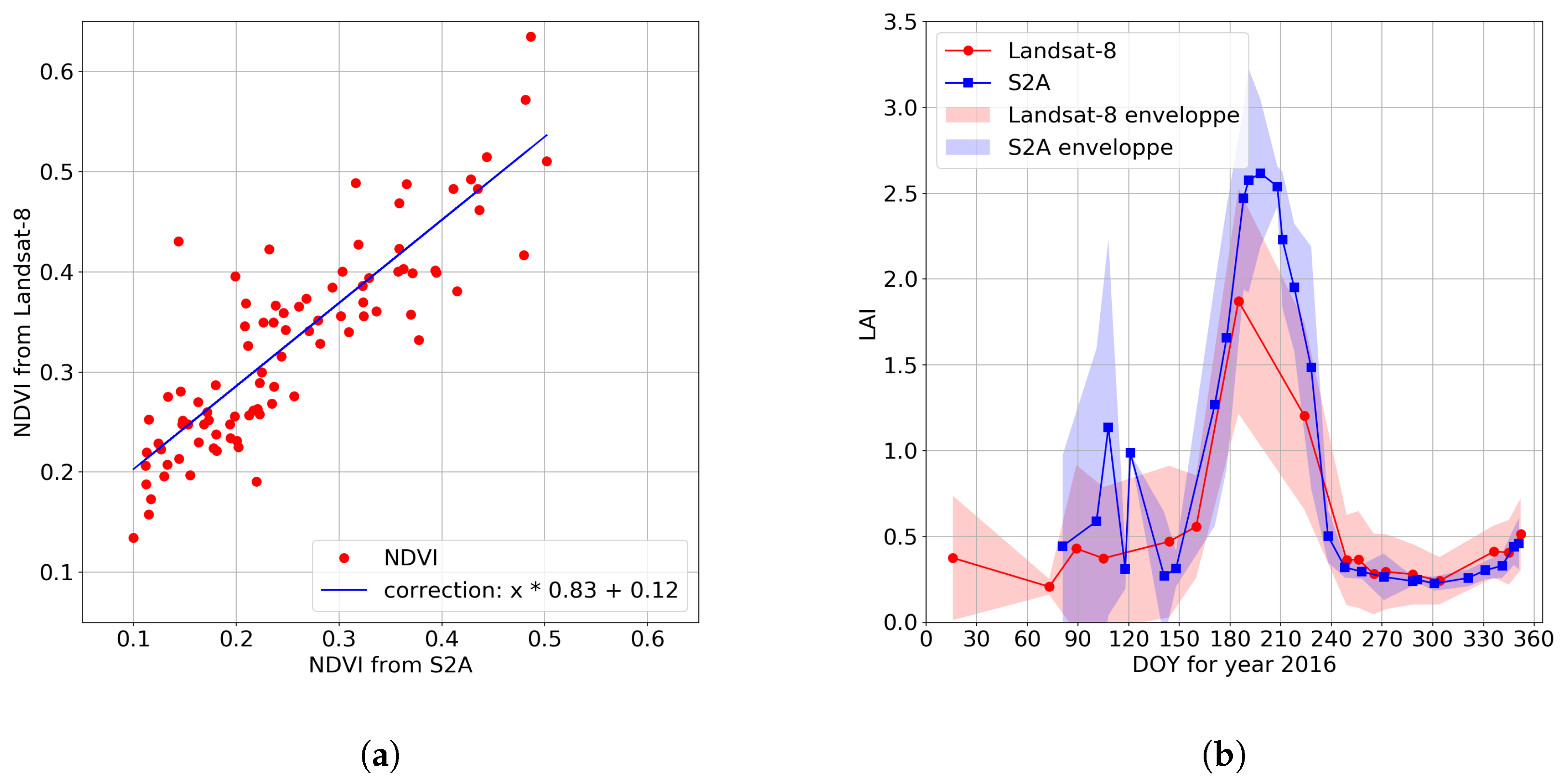
Based on the dates of simultaneous acquisitions, the NDVI from Landsat-8 and Sentinel-2A are compared. Figure 2a shows the scatter plot between the mean over each plot of the NDVI from Landsat8 and from Sentinel-2A. It also shows the correction function that was used to convert the Sentinel-2A NDVI to Landsat-8 like NDVI. The corrected NDVI is used to obtain the Sentinel-2A LAI using an exponential function (Equation (1)) that was fitted between the Landsat-8 NDVI and Landsat-8 LAI (with an R = 0.98). Figure 2b shows the final time series of homogenized Sentinel-2A and Landsat-8 LAI with the corresponding envelope area obtained from the standard deviation across all field plots.
L A I = 0.1388 exp ( 3.711 N D V I ) 0.17
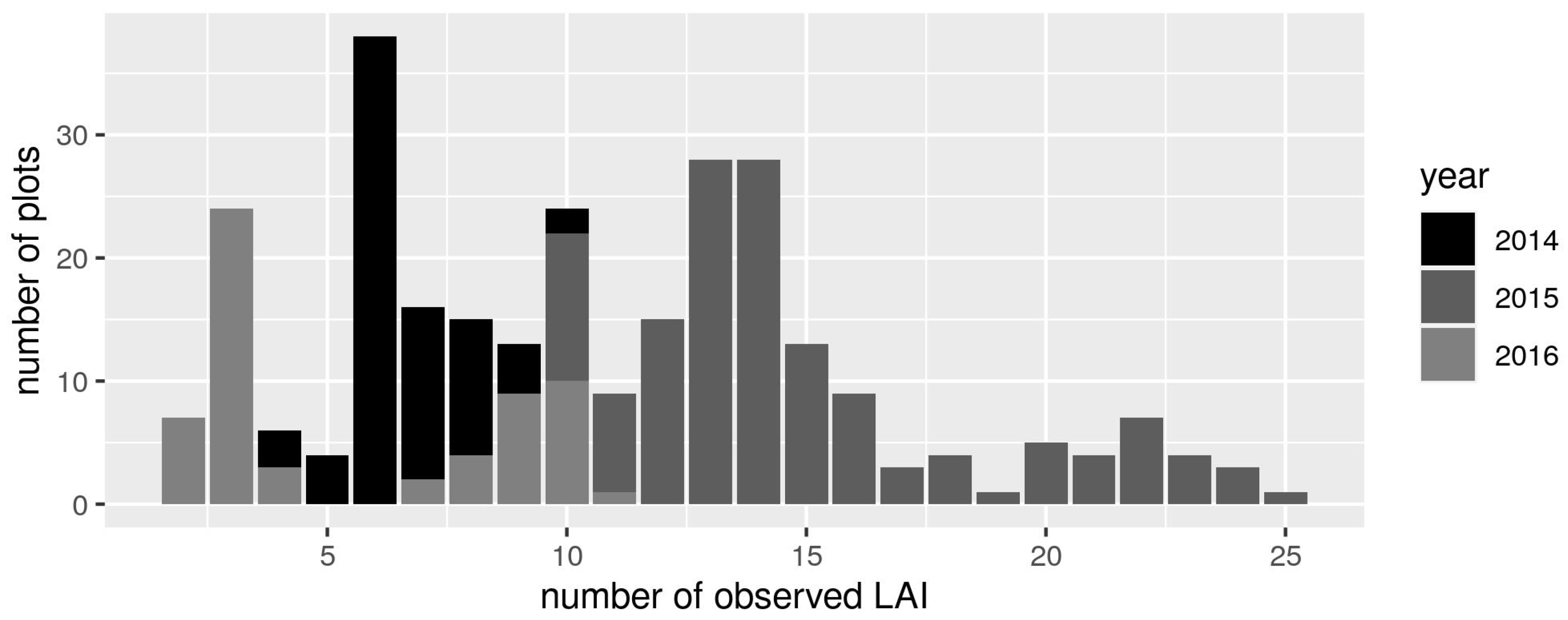
As a result, after processing the images from all the sensors, the mean number of observed LAI per plot that remained during the sunflower growing season (from May to August) was 10.64 with a range of 2 to 25 (Figure 3). The number of images was essentially depending on the cloudiness, 2015 being a dry and shiny year.

2.3. Crop Simulation with SUNFLO

SUNFLO is a process-based model for the sunflower crop which was developed to simulate the grain yield and oil concentration as a function of time, environment (soil and climate), management practices (irrigation, nitrogen fertilization, crop density) and genetic diversity, through genotype-dependent inputs [18,19].
The model simulates the main soil and plant processes: root growth, soil water and nitrogen content, plant transpiration and nitrogen uptake, leaf expansion and senescence and biomass accumulation, as a function of main environmental constraints (temperature, radiation, water and nitrogen deficits).
This crop model is based on a conceptual framework initially proposed by Monteith [26] and now shared by a large family of crop models [27,28,29,30]. In this framework, the daily crop dry biomass ( T D M t , g·m 2 ) is calculated as an ordinary difference equation (Equation (2)) function of incident photosynthetically active radiation (PAR, MJ·m 2 ), light interception efficiency ( 1 e k . L A I ) and radiation use efficiency (RUE, g·MJ 1 [31]). The light interception efficiency is based on Beer–Lambert’s law as a function of leaf area index ( L A I ) and light extinction coefficient (k).
T D M t = T D M t 1 + R U E t ( 1 e k L A I t ) P A R t
The soil model describes root growth, water flux and extraction, and nitrogen absorption and mineralization. Crop management is described by the sowing date, plant density, timing and amount of nitrogen fertilization and irrigation. Detailed algorithms and equations of SUNFLO can be found in [18,19]. The oil model was recently refined by [32]. A more complete description of the crop model was published as additional data in [33].
The model inputs (Table 2) are soil properties and initial conditions, cultivar features and technical operations (irrigation, fertilization). Daily weather data are also needed for simulation and are composed of five variables commonly available in weather stations: maximum and minimum air temperatures (T, C), precipitation (P, mm), potential evapotranspiration (PET, mm), global radiation (GR, MJ·m 2 ).
Nine soil inputs are needed to describe the soil depth available for roots, its water holding capacity and initial soil conditions at sowing. Each variety is described by 11 inputs, whose values for the considered varieties were previously measured in independent experiments.
There was a focus on nine state variables particularly involved in yield prediction in data assimilation methods. Two were related to the crop aerial part: LAI and total dry biomass (TDM, MJ·m 2 ). Two were related to soil properties: water content in the two soil layers (C1 and C2). The last five were related to the plant–soil interaction: root depth (zRac, mm), water deficit index (FTSW), nitrogen deficit index (INN), cumulated transpiration between the flowering and the maturity stages (TRPF, mm), absorbed nitrogen (Nabs, kg·ha 1 ).

2.4. Sensitivity Analysis

Sensitivity analysis is generally used to identify input factors that have a large influence on model outputs [34]. The aim of this study was to forecast the grain yield using both the SUNFLO model and the measurements of LAI, so it seemed relevant to identify which are the input factors that influence both grain yield and LAI. In the SUNFLO model, the soil conditions at sowing (initial water and nitrogen content) as well as more permanent soil properties (soil texture, stone content, bulk density and rootable depth) define the water deficit which is the main limiting factor for crop growth. The simulated water deficit is also impacted by management options (variety, plant density, nitrogen fertilization, irrigation) and weather conditions (temperature, precipitation, radiation). This information is generally easier to get from surveys and databases although some residual error exists (e.g., distance from the weather station, inaccuracies in input timings and amounts).
To identify the most important input factors, a screening approach has been conducted using the Morris method [35] on both the maximal value of LAI (at flowering) and the grain yield. The Morris method, by using intensive simulations, computes two indices for all screened input factors: μ and σ . For a given input factor, these indices are expressed in the unit of the output variable (either grain yield or LAI in our case) and aggregate elementary effects. An elementary effect is the absolute difference of output value due to the difference in the value of one solely input. The  μ index represents the overall linear influence of the input on the output and σ is the non-linear influence of the input plus the influence of its interaction with other inputs.
As a result that the impact of input factors depends on environmental conditions, two contrasted production situations were considered for the sensitivity analysis. They differed from each other by climate data and management but both are located at ’En Crambade’ near Toulouse on clay soil.
  • Low production level: dry weather (2005), no nitrogen fertilization, low plant density (4.5 plants·m 2 ), early-maturing cultivar.
  • High production level: wet weather (2002), application of 80 kg·N·ha 1 , high plant density (6.5 plants·m 2 ), late-maturing cultivar.
For most of the situations in this project, uncertainty on collected input values was not available. Consequently, a variation of 30% of the inputs around the default value is considered. Constraints on some of the inputs in order to keep some realism in the simulations were required:
  • w a t e r I n i t i a l and s t o n e C o n t e n t , which are fractions, were kept between 0 and 1.
  • r o o t D e p t h ranged between 400 and 2000 mm according to our expertise on soil heterogeneity in the Toulouse region.
The range of variation of inputs for the two situations was given in Table 3.

2.5. Data Assimilation

Three alternative options for assimilating remote sensing data into the SUNFLO crop model are considered in this work. They are all detailed in Appendix A.
The simplest method consists of direct insertion (DI) of the value of LAI into the crop model each day an observation is available. The assumption is that the total dry biomass (TDM) that is closely related to grain yield will be updated by propagation of the observation through the simulation equations. An example of the resulting LAI dynamics is illustrated on a plot of our dataset in Figure 4.
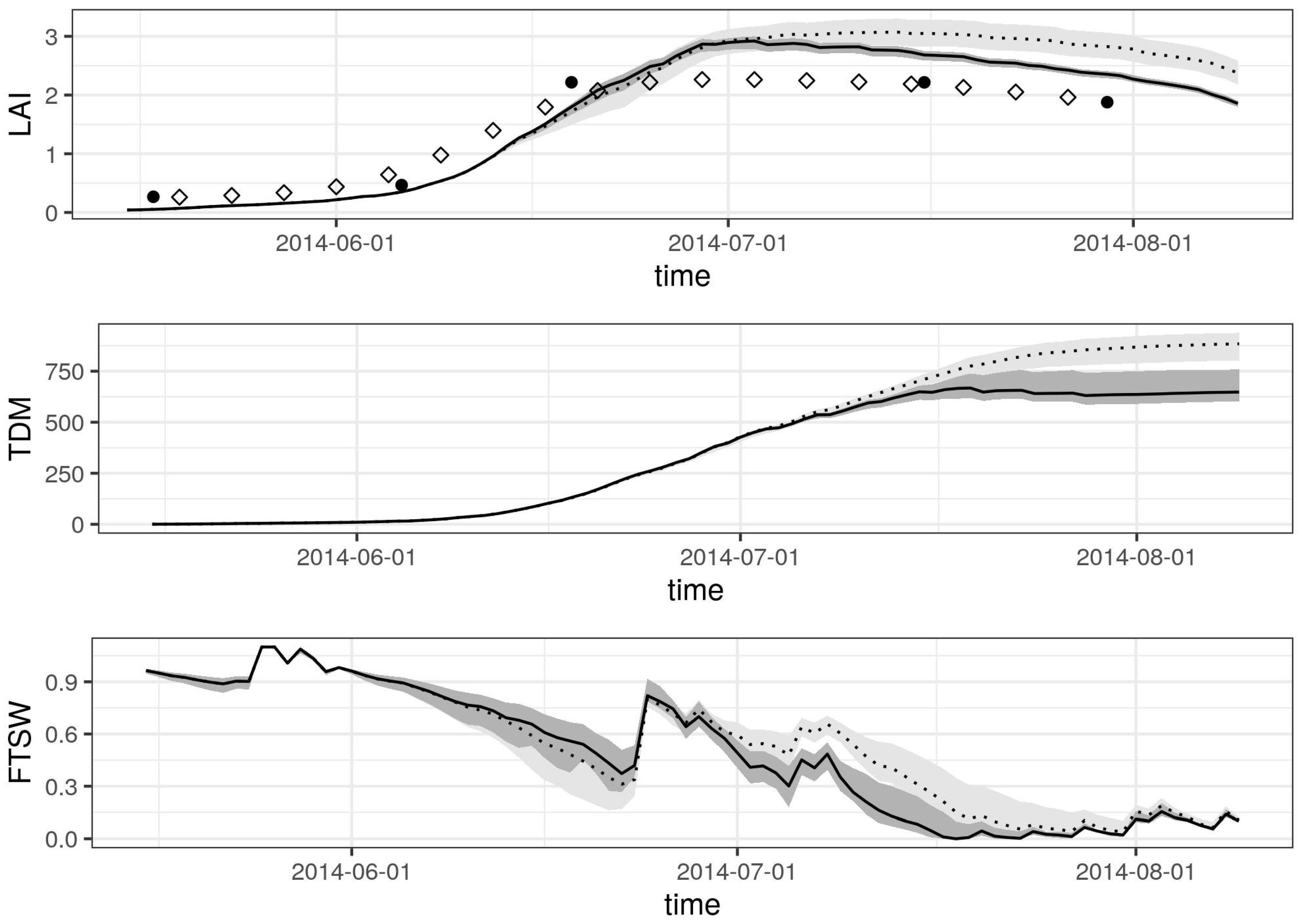
A more sophisticated update scheme is the ensemble Kalman filter (EnKF). Rather than updating only the LAI variable into the system at days of observations, nine state variables (defined in Section 2.3) are updated according to a covariance matrix of these variables. It is assumed that the state variables vector is a random variable with a multivariate normal distribution. The EnKF relies on the simulation of different model states in order to update the covariance matrix at each day of observation. In our case, the different model states correspond to different initializations of soil conditions. At the day of forecast, the model state corresponding to the median value of total dry matter (TDM) is selected. An example of this method for a subset of three state variables is presented in Figure 5.
Re-estimating input factors is another way of assimilating LAI from remote sensing. One can seek for the least square estimator (LSE) of soil conditions, by comparing simulated and measurements of LAI. It consists of finding the soil conditions that lead to the minimal sum of squared errors of the variable LAI. It requires an optimization method for solving the minimization problem. It is noteworthy that, additionally to the updated model state at the day of forecast, the LSE approach provides new estimates of the soil conditions. An example of the resulting LAI is illustrated in Figure 4. Inputs that were re-estimated were selected within the candidate list (Table 2) by the sensitivity analysis step.
The data assimilation methods provide an estimation of the crop model state at the days of forecast. To complete the simulations in order to get an estimation of the grain yield, the crop model requires weather time series between the day of forecast and the harvesting day. In an operational context, the true weather series are not known. Instead, the past weather series at the location of the study plot (24 previous years) were used for the completion of the simulation.
Before the assimilation, the sequence of LAI can be smoothed in order to extract more frequent observations. Li et al. [36] used a Savitzky–Golay filter in order to smooth the noise of LAI time series imagery. Here the Whittaker method is carried out as proposed in [37] which behaves well for vegetation indices when compared to other smoothing techniques [38]. Compared to other methods, it has the advantage to be suitable for handling partial LAI sequence. Indeed, in our case, the whole sequence cannot be available, since the time of forecast (set to August 10th) is before the time of harvesting.
In a nutshell, two alternatives were considered for the preprocessing of LAI from remote sensing.
  • raw LAI: no preprocessing is performed on measurements of LAI.
  • smoothed LAI: LAI values were extracted at constant time intervals from a smoothed sequence of LAI using the Whittaker smoother.
A direct simulation and three approaches for assimilating LAI measurements were compared in this paper, details are given in Appendix A:
  • Open-loop simulation: a direct simulation with no LAI forcing.
  • Direct insertion (DI): the simplest assimilation method that consists in replacing the model LAI state variable at each time of observation.
  • EnKF: the ensemble Kalman filter method.
  • LSE: the least square estimator.
Additionally two different sets of weather series used for completing the simulation were compared:
  • oracle (for comparison purpose): the true unknown weather series is used for the simulation between the day of forecast and the harvesting day. It is impracticable in an operational context but can be used to assess the impact of weather variables during this time interval.
  • past weather: 24 past years weather series, at the location of the plot, are used to complete the simulation from the day of forecast to the harvesting day. The forecast grain yield is the average of the 24 simulations of grain yield.

2.6. Experiments Settings and Software

The crop model SUNFLO and the EnKF method were implemented in C++ (gcc 5.3.0) with the VLE software version 2.0 [39] using the modeling platform RECORD [40] and the eigen library version 3 [41]. The rest of the experiments were performed with R version 3.6.1 [42]. Crop model simulations and optimization (∼2M simulations) were performed on the muse cluster (Montpellier University).
For the sensitivity analysis, the Morris method with parameter values r = 100 and l e v e l s = 5 from the R packages sensitivity [43] was used. That consists in 2400 simulations for each sensitivity analysis. To smooth LAI observations, the implementation of the Whittaker smoother in the R package pracma [44] with the parameters l a m b d a = 500 and d = 2 was mobilized, and LAI were extracted from the smoothed sequence every four days. No setting was required for the open-loop simulation and the DI methods. For the EnKF method, 100 particles were simulated ( M = 100 in Appendix A) and an error variance of the LAI observation was set to 0.2 ( R = 0.2 in Appendix A). For the LSE approach, the genetic optimization algorithm genoud [45] from the package rgenoud (version 5.8) was used with 50 generations and a population of size 16 for each optimization.

3. Results

3.1. Sensitivity Analysis of SUNFLO Crop Model

The variation of simulated maximal LAI and grain yield corresponding to sensitivity analyses were important (Figure 6), indicating that the uncertainties in input conditions had a strong impact on considered output variables. Indeed, the relatively high uncertainty obtained on the input conditions lead to a very high variation in grain yield, from 7 to 44 q·ha 1 for the low production level situation and from 11 to 46 q·ha 1 for the high production level situation. As expected, the difference in simulated grain yield between the two situations is statistically significant (with a p-value p < 2.2 × 10 16 in the non-parametric Wilcoxon test).
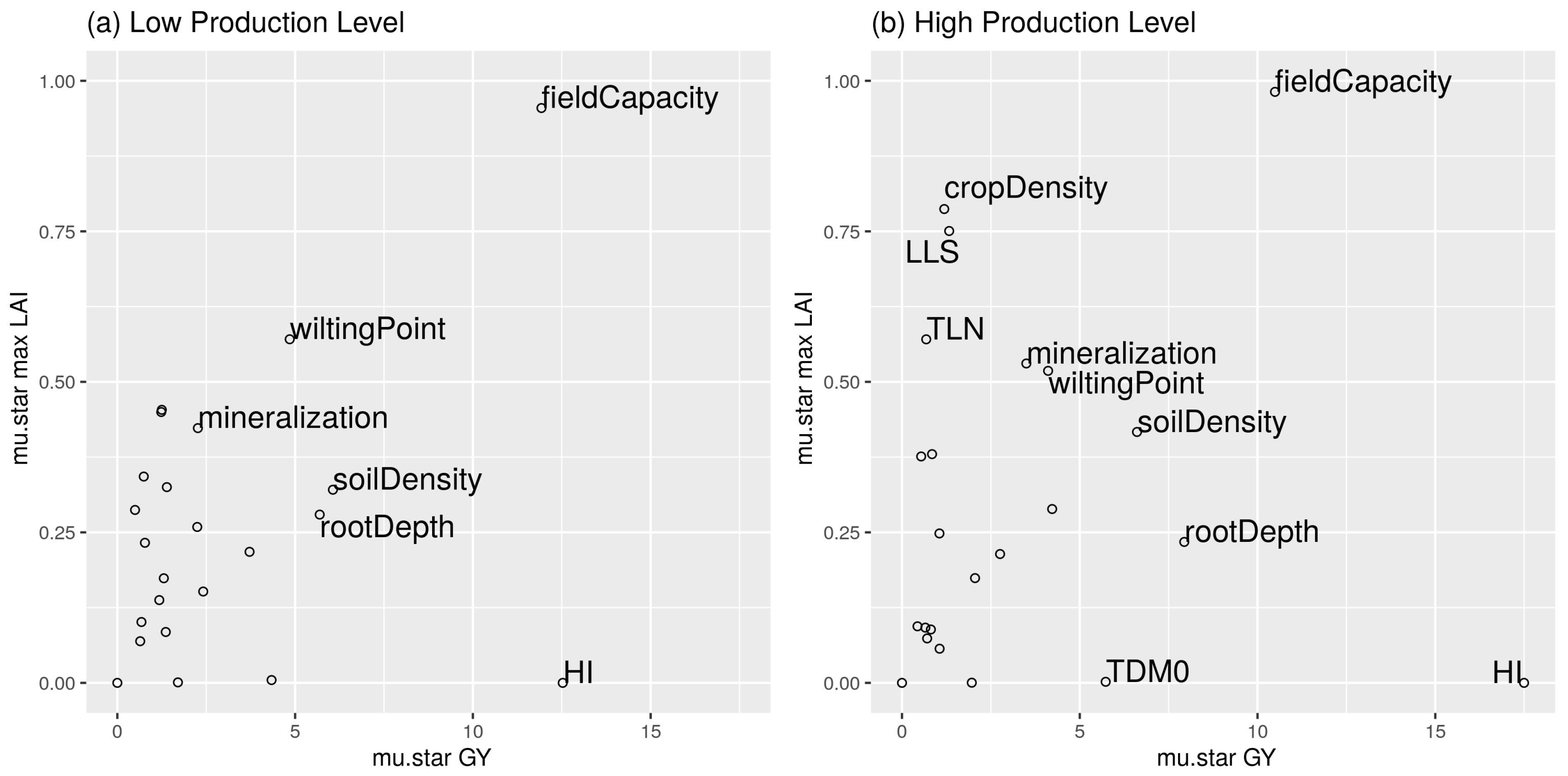
From these experiments, the means of absolute elementary effects (mu.star) resulting from the Morris method for both the maximal LAI and yield are shown in Figure 7 for the two contrasting production situations. These indices allowed the selection of the most impacting input factors on LAI and yield output variables. Components which were used for the calculation of the soil water capacity (and consequently the calculation of the water deficit) mostly impacted the LAI and grain yield: this was the case for f i e l d C a p a c i t y , w i l t i n g P o i n t , s o i l D e n s i t y , m i n e r a l i z a t i o n and r o o t D e p t h , especially the input f i e l d C a p a c i t y for both situations. However, w a t e r I n i t i a l and s t o n e C o n t e n t were not relevant for further selection. In our conditions, the permanent soil properties that determined soil water capacity and nitrogen mineralization were more relevant to select than variables describing the initial conditions at sowing time.
The inputs related to plant features such as the individual maximum leaf area ( L L S ), the potential number of leaves at flowering ( T L N ) and the crop density had a strong impact on maximal LAI but a lower impact on the yield. Thus re-estimating them in the LSE approach, or randomizing them in the EnKF approach, would not be of interest for improving yield forecasts. Conversely, a variation of H I (potential harvest index) resulted logically in a high variation of yield. However, as expected, it did not impact the simulated LAI since H I intervenes after the peak LAI during the crop development. Re-estimating H I using LAI measurements as a proxy would not be relevant.
Despite the fact that soil conditions are difficult to acquire on farms, these results confirmed that they impact strongly the simulated crop production. This validates the main hypothesis of this work. Therefore, these inputs are good candidates for modeling input conditions’ uncertainty into the data assimilation process. As a result, the randomized input factors selected for LSE and the EnKF approaches are the five soil input conditions: f i e l d C a p a c i t y , w i l t i n g P o i n t , s o i l D e n s i t y , m i n e r a l i z a t i o n and r o o t D e p t h .

3.2. Data Assimilation Results

Table 4 gives a global overview of the evaluation criteria for the performance of the assessed yield forecasting approaches, over the 281 sampled plots. Bias, root mean squared error (RMSE), normalized RMSE (RRMSE) which is the RMSE divided by the mean of the observations, mean absolute error (MAE) and the coefficient of determination (R2) are listed for all the combinations of the different methods. As a reminder, this evaluation encompasses the effects of the assimilation method (open-loop simulation, direct insertion, the ensemble Kalman filter and least square estimator), the weather series used to complete the simulation (‘oracle’ or ‘past weather’) and the LAI variables used during the assimilation process (‘raw LAI’ or ‘smoothed LAI’).
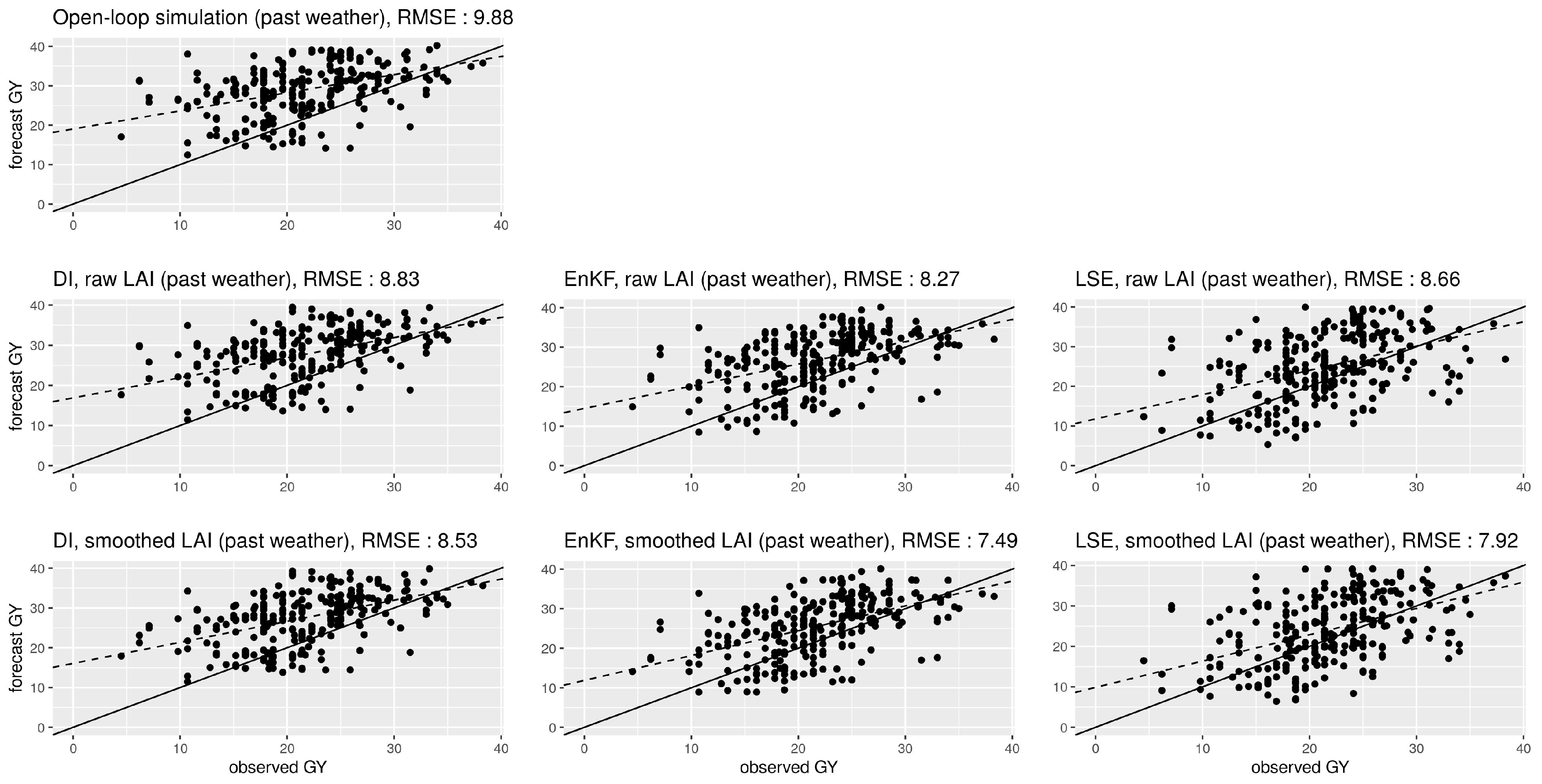
Relying on LAI measurements to forecast the grain yield led to better results than the simulation alone, regardless of the assimilation approach and the criterion. The best results in terms of R2 and RMSE are obtained by using the EnKF approach with smoothed LAI and the best results obtained for the bias was the LSE with smoothed LAI. Figure 8 shows the forecast yield as a function of observed yield for all the methods based on the used of past weather series, as well as the the reference prediction (no assimilation).
However, these approaches resulted in overall poor performances for the sampled field population. The model largely overestimated plot yields in the reference simulation (bias is 7.33 q·ha 1 ) with a relatively low correlation (R2 is 0.18 ). As a result, the assimilation of LAI in order to improve yield forecasts resulted mainly in bias reduction. The LSE approach performed best for this criteria (bias reduction up to 2.4 q·ha 1 using the smoothed LAI), but the correlation between the observed and forecast yields with LSE was low.

3.2.1. Impact of the Use of Past Weather Series

To achieve a complete simulation, a daily weather series is necessary from the day of forecast to the harvesting time. Available past weather series at the location of the plot were used to complete the simulations. The impact of this choice was assessed by comparing the ‘oracle’ alternative and the ‘past weather’ dataset. In the ‘oracle’ dataset, the actual unknown weather series was used to complete the simulations.
The mean absolute difference of yield forecasts based on the ‘oracle’ alternative on one hand, and the ‘past weather’ alternative on the other hand, was only 0.02 q·ha 1 and was not statistically significant (with a p-value p = 0.15 in the non-parametric paired Wilcoxon test). The maximal difference, over the 281 plots, between the two alternatives was also very low ( 1.4 q·ha 1 ).
Therefore, one can conclude that the final yield value was nearly independent of the weather inputs after the day of forecast, which was set to August 10th in this study (about one month before harvest). Thus, the rest of the analysis was based on the ’past weather’ alternative which corresponded to the practicable approach.

3.2.2. Forecasting Methods Comparison

The difference in mean absolute error (MAE) was computed for all pairs of methods to provide a side-by-side comparison in Table 5. Given two methods, the non-parametric paired Wilcoxon test was also performed on individual absolute errors to analyze, over the 281 situations, the significance of the difference in MAE.
As in Table 4, it is shown that using both LAI measurements and simulation provided better forecasts than the simulation alone (all the differences in MAE were significant). The EnKF approach with smoothed LAI led to significantly better predictions than all the other ones, except for the LSE approach with smoothed LAI. Using smoothed LAI, even if it was not significant, the EnKF approach led however to better MAE than the LSE method (a difference of 0.275 q·ha 1 ).

3.2.3. Impact of Smoothing LAI

There was a significant difference between assimilating raw LAI and assimilating smoothed LAI ( 0.84 q·ha 1 with a p-value p = 9.5 × 10 22 in the non-parametric paired Wilcoxon test). Moreover, the maximal difference between the two alternatives was high (21 q·ha 1 ). These results emphasized the important improvement when using smoothed vegetation indices with the Whittaker smoother during the data assimilation process. Smoothing LAI led to an improvement of the forecast accuracy of 3.39% of RMSE for direct insertion, 9.43% for the ensemble Kalman filter and 8.54% for the least square estimator (see Table 4). Most sophisticated methods (i.e., EnKF and LSE) are more sensitive to the frequency of observations in the LAI time series. In view of these results, the rest of the analysis focuses on assimilation approaches of smoothed LAI.

3.2.4. Impact of Yield Limiting Factors

To further analyze results with an agronomic point of view, the crop monitoring data that were collected during the growing season on each field was mobilized: the fraction of field area infested by weeds or concerned by severe irregular plant population, and the fraction of plants severely attacked by fungal diseases (e.g., phomopsis, phoma, verticillium).
Situations were considered out of the validity domain of the simulation model (i.e., yield was limited by factors not included in the model) when weeds were covering more than 25% of the area, when yield loss expected from disease survey was more than 3 q·ha 1 , or if the field had important areas without plants. Based on this categorization of the 281 plots, the methods were compared with respect to the different yield limiting factors (Table 6).
The population of fields (with or without the observed limiting factors) was split and model statistics were operated on each of the groups. First, a yield limiting factor has been observed in most of the fields: 263 amongst 281 corresponding to 93% of the plots.
The best yield prediction was achieved on the subset of fields without limiting factors, with the prediction error increasing with added limiting factors. This can be explained by the fact that biotic limiting factors are not modeled into the SUNFLO crop model and by the fact that crop density used as input variable of the model did not consider the fraction of the field occupied by weeds.

4. Discussion

In this study, it has been shown that the availability of accurate soil conditions for the SUNFLO crop model is of crucial importance for yield simulation. The performed sensitivity analysis confirmed the high impact of soil conditions on simulated yield and leaf area index, which is in line with previous works on other crops and other crop models [1,2] and validated these inputs as good candidates for calibration in a data assimilation process. This result was expected as sunflower crop is grown as a rainfed crop in southwestern France, in a context of high summer evaporative demand and moderately deep soils. As stated, water is the main limiting factor for production of sunflower in the region [46].
Statistically significant improvement was achieved in yield forecasting by assimilating LAI from remote sensing into the sunflower crop model SUNFLO, compared to simulation alone. Moreover, using a past weather series instead of the true series to complete the simulation between the day of forecast (set about one month before the harvest) and the harvesting day did not impact the quality of results. This suggests that, in the context of cooperatives needs in southwest France, forecasting sunflower yield one month before harvesting is not a limit for a precise estimation.
Regardless of the method used, the yield forecast was improved by the most sophisticated methods, i.e., calibration (LSE) and ensemble Kalman filter (EnKF). Although these two types of methods are used in the literature [15], they were rarely compared side-by-side. Here, the ensemble Kalman approach performed better (except for bias criteria) but this result is difficult to extrapolate since yield forecasts obtained by simulation alone were not precise enough yet.
Indeed, the main limitation in the assessments of these assimilation approaches is the mismatch between the open-loop simulation results and the field observations (yield and LAI). In the fields sampled in this study, a bias of 7.3 q·ha 1 was obtained whereas the expectations of agronomists and cooperatives in terms of performance is estimated at less than 3 q·ha 1 one month before harvesting. In sunflower, only a few papers refer to the use of remote sensing to predict sunflower yield. They differ by the nature of the actual data used for evaluating the performance of the model when assimilating remote sensing data: yield either at regional, farm, field or intra-field level, yield information from the farmer or directly measured by sensors onboard harvesters. Semi-empirical models as SAFY [17] and SAFY-CO2 [47] or statistical models (linear models, non-parametric approaches, etc.) based on the use of NDVI, LAI or leaf area duration were also evaluated for yield prediction [48,49]. In spite of these differences in methodological approaches, the RMSE was mostly ranging from 4 to 6 q·ha 1 which is close to the performance of SUNFLO used in assimilation with the EnKF approach in conditions with no major limiting factors (5.8 q·ha 1 ) but with more uncertainties on the observed yield values.
In our experiments, when LAI measurements from remote sensing are used in a data assimilation approach, the improvement of the model prediction error is still required. One frequent explanation for poor performances of crop models when applied on-farm is that they do not take into account various yield reducing factors associated with pests or weeds or uneven plant stand. By assimilating LAI from remote sensing, the effect of these factors on leaf growth were partially accounted for. Others factors such as fungal diseases (e.g., fungal phoma, phomopsis) reduce yield not only by impacting leaf area and radiation interception, but also through a reduction of radiation use efficiency. In this case, the assimilation approach could not correct such indirect effects as the remote-sensed variable carries no information about it.
In these circumstances, the risk of assimilating LAI observations is to compensate for the lack of representation of unfavorable soil properties. In these experiments, this is especially true for the least square estimator (LSE) approach when one seeks to re-estimate soil properties. The calibration of the SAFY model for the sunflower crop near Toulouse has been performed from remote sensing in [17]. The researchers emphasized that the estimated harvest index (0.25) was significantly lower than the potential harvest index considered in SUNFLO (from 0.32 to 0.51 according to varieties). This can explain the over-estimation of yield forecast and constitutes a line of thought to improve the SUNFLO model in the context of on-farm experiments. However, the model accuracy on fields without non-modeled yield limiting factors was in the range of previous independent experimental validations (RMSE 4–7 q·ha 1 ) as reported in [18,50,51,52].
One solution for providing relevant yield estimates is to consider agronomic models that are forced by remote sensing LAI without the introduction of the water stress derived from the soil moisture availability in the context of a least square estimation. In this case, the impact of low water content availability can be compensated by the frequent observation of vegetation phenology. This solution still has two major drawbacks: first its inability to provide a consistent set of soil/vegetation outputs which means that water needs cannot be estimated, and second it needs to be applied on full crop cycle because the impact of water stress on LAI presents a lag in time.
Finally, smoothing the LAI before the assimilation leads to significantly better results. This point is largely discussed in other approaches involving only remote sensing observations [36], and not really in a crop model based data assimilation approach. Extracting an estimation of LAI every four days from the smoothed sequence facilitates the data assimilation in our experiments where only 7 to 13 images are available yearly. The main advantage of the smoothing pre-process is to provide relevant LAI with a reduced number of acquisitions. It is also foreseen that the increased availability of LAI from optical sensors like Sentinel-2 and proxy-LAI from Synthetic Aperture Radar data like Sentinel-1 from the European Union Copernicus program will enable high temporal frequency of LAI even in cloudy weather. Considering that smoothing LAI reduces the uncertainty of the dataset and corrects for satellite acquisition configurations and sensor differences of the LAI dynamics, except for very extreme events (fire, hail, etc.), it should remain of interest to use this type of filter.

5. Conclusions

The goal of this study was to investigate the relevance of data assimilation of remote sensed LAI into the SUNFLO crop model in order to forecast sunflower grain yield about one month before harvest. Three approaches were considered: the direct insertion of remote sensed LAI into the crop model, an ensemble Kalman filter approach and a least square estimator approach. A preliminary sensitivity analysis of the crop model was performed to identify the crop model inputs that influence the most the simulations of LAI and grain yield. The impact of smoothing the remote sensed LAI before the assimilation, using a Whittaker smoother, was also assessed. Experiments were conducted near Toulouse, southwest France, on a total of 281 fields monitored over three consecutive years (2014–2016).
The sensitivity analysis emphasized the impact of soil available water on simulated LAI and grain yield. Assimilating smoothed remote-sensed LAI using an ensemble Kalman filter led to the best improvement in adequacy between forecast and observed grain yield. The least square estimator of available water components led also to an important improvement of this adequacy. A significant conclusion of these experiments is the beneficial role of smoothing LAI beforehand the assimilation.
This study also underlined the need for crop model adaptations for on-farm use cases, since grain yield was overestimated because of the occurrence of limiting factors such as weeds and diseases. For weeds, it would be interesting to rely on remote sensing techniques that allow to identify the ratio of weeds and crops dynamically [53,54]. This could be taken into account in the assimilation process by re-estimating the covering of the crop. On the contrary, identifying the whole disease injuries by remote sensing seems to be challenging and including fungal disease into the modeled system would be a relevant strategy.
To go beyond the grain yield forecasting, agricultural cooperatives need also estimations of the oil content, which is simulated by the crop model SUNFLO as well. Even if sunflower oil content is mainly determined genetically by the crop variety, it is also impacted by the post flowering photosynthetically active radiation and by the LAI dynamics [55]. Thus, assimilating LAI in SUNFLO in order to forecast the sunflower oil content should be feasible.
Finally, one of the main theoretical drawbacks of the ensemble Kalman filter is its inability to handle non Gaussian distributions of state variables. To avoid this assumption, one can rely on a Bayesian framework for data assimilation, as in [14], in which a particle filter was implemented. Nevertheless, as suggested in [4], the re-sampling method, such as sequential importance sampling, that is required in the particle filter approach, would benefit a stochastic version of the crop model.

Author Contributions

Conceptualization: R.T., L.C., J.-F.D., A.A.B., P.C., P.D.; methodology: R.T., L.C., J.-F.D., A.A.B., P.C., P.D.; software: R.T., J.-F.D., P.C.; validation: R.T., L.C., J.-F.D., A.A.B., P.C., P.D.; formal analysis: R.T., A.A.B.; writing—original draft preparation: R.T.; project administration: L.C., P.D. All authors have read and agreed to the published version of the manuscript.

Funding

The authors are grateful for the funding of this research by the two projects: CASDAR 1311 2014–2016 (French Ministry of Agriculture) and PROMISES 2018–2020 supported by Carnot Plant2Pro (French National Research Agency).

Acknowledgments

The authors thank Arterris and Val de Gascogne for their help in structuring the field network. They also thank A. Micheneau, H. Gibrin, B. Garric, Y. Fernandez and F. Attia for their work on this project. R.T. additionally thanks A. C. Ruane (NASA Goddard Institute for Space Studies) for his comments on this work. This work has been realized with the support of the High Performance Computing Platform MESO@LR, financed by the Occitanie Region, Montpellier Mediterranean Metropole and the University of Montpellier.

Conflicts of Interest

The authors declare no conflict of interest. The funders had no role in the design of the study; in the collection, analyses, or interpretation of data; in the writing of the manuscript, or in the decision to publish the results.

Abbreviations

   The following abbreviations are used in this manuscript:
NDVInormalized difference vegetation Index
LAIleaf area index
GYgrain yield
TDMtotal dry matter
FTSWfraction of transpirable water
DIdirect insertion of LAI
LSEleast square estimator
EnKFensemble Kalman filter
R2coefficient of determination
MAEmean absolute error
RMSEroot mean square error
DSSATdecision support system for agrotechnology transfer
CEREScrop environment resource synthesis
SAFYsimple algorithm for yield
STICSsimulateur multidisciplinaire pour les cultures standard
SUCROSsimple and universal crop growth simulator
SWAPsoil-water-atmosphere-plant
WOFOSTworld food studies

Appendix A. Data Assimilation Methods

In order to formally describe the forecast approaches, some notations are required. Let U = { f i e l d C a p a c i t y , w i l t i n g P o i n t , s o i l D e n s i t y , m i n e r a l i z a t i o n , r o o t D e p t h } be the set of input parameters that are randomized into the data assimilation process. The choice of U relies on sensitivity analysis results in Section 3.1. Let X R | | U | | , with | | U | | the length of U, be the range of variation of inputs U as described in Section 2.4. There is an assumption that into X , lies the true input combination x and let x b (b stands for ‘background’) be the input values from data collection. Let L A I 1 , . . . , L A I N 1 be the LAI observations given by remote sensing techniques (either smoothed or not) at times t 1 , . . . , t N 1 , respectively. Let t N be the day of forecast and t N + 1 the harvesting date. Times t 1 , . . , t N + 1 are in increasing order. Let Y be the model state domain, and  y [ L A I ] be the LAI component of the state y Y . One considers that the model provides a simulation function f and an initialization function g:
f : X , Y , { t 1 , . . . , t N } , { t 2 , . . . , t N + 1 } Y
g : X Y
The function f is the model state transition between two clocks. Hence, f ( x , y , t i , t j ) , simulates the model state to time t j starting from time t i with an initialized state y using input values x . The function g models the initialization of model states at t 1 , which depends on the input combination under which simulation is performed.
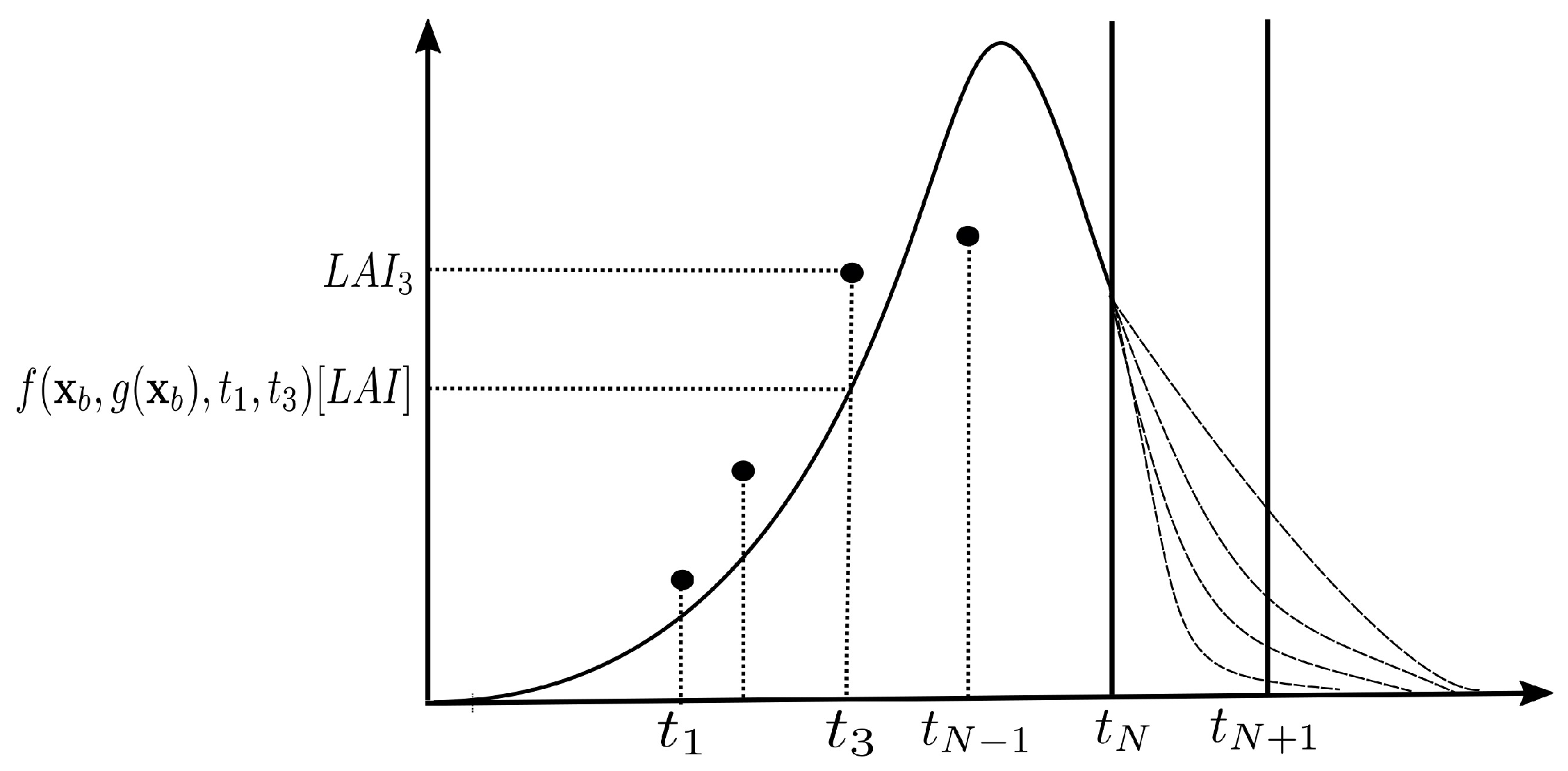
The different assimilation methods consists of providing a corrected model state y ^ N at the day of forecast. One relies on observations { L A I 1 , . . . , L A I N 1 } , the  input uncertainty modeled by a uniform distribution on X and the use of simulator f until the day of forecast t N . The problem is illustrated in Figure A1.
Figure A1. Notations used in the problem formulation. To improve grain yield forecast, both LAI observations from remote sensing (e.g., L A I 3 ) and a simulator function f are used to provide a new model state at the day of forecast t N .
Remotesensing 12 03816 g0a1
The open-loop method provides an estimation of y ^ N by using the simulation of SUNFLO until t N with background inputs values x b without taking into account neither its uncertainty nor the LAI observations. Formally, it can be written as:
y ^ N = f ( x b , g ( x b ) , t 1 , t N )
The purpose of this method is to provide a base for comparison with other methods. Figure 4 illustrates the simulation for a specific plot.
The direct insertion (DI) method (Algorithm A1) for estimating y ^ N is to simulate SUNFLO until t N without taking into account the uncertainty of input values, one thus relies on the input values from data x b . The LAI state is forced to take the observation values during simulation at the different times of observations. An illustration is given in Figure 4.
Algorithm A1 Direct insertion (DI) method for LAI assimilation
Remotesensing 12 03816 i001
The EnKF method (Algorithm A2) consists in using an ensemble Kalman filter (EnKF) to combine LAI observations and simulations, covariance error of observations R and the covariance of state variables B i at each time of observation t i . The optimization problem can be formulated, for each observation time t i , into the 3Dvar paradigm of data assimilation, as this function for updating y :
y ^ i = argmin y | | y f ( x b , y ^ i 1 , t i 1 , t i ) | | B i 1 + | | L A I i h T y | | R 1
The vector y ^ i is called the analysis state and is used to force simulation state at time t i . The vector f ( x b , y ^ i 1 , t i 1 , t i ) is called the background state which is basically the simulation of the model from t i 1 to t i starting from the previous analysis state, computed at time t i 1 . The vector h is the observation operator. In our case, the observation is directly linked to the LAI model state variable and h is 1 at the index of the LAI variable and 0 otherwise. Thus, h T y = y [ L A I ] . Whereas the ensemble Kalman filter does not address directly the optimization problem, it is suitable to produce an estimation of y ^ N by considering the state covariance B and the error covariance R . It maintains simultaneously the simulation of M particles to estimate B . The M particles are initialized with uniform random input values into X .
Algorithm A2 EnKF for L A I assimilation
Remotesensing 12 03816 i002
Figure 5 is an illustration of the use of assimilation by ensemble Kalman filter to assimilate, until t N , LAI observations into the SUNFLO model. Once we have y N m for each particle, the corrected state y ^ N is defined as the state of the particle with the median value of TDM at t N .
Finally, the least square estimator (LSE) of x is given in Equation (A4). Using an optimization method, the soil conditions are re-estimated. Then, by simulating the LSE until t N , we obtain an estimation of y ^ N . Compared to the EnKF approach, the LSE provides also an estimation of x . An illustration of the LSE method results is given in Figure 4.
x ^ = argmin x X 1 N 1 i = 1 i = N 1 ( L A I i f ( x , g ( x ) , t 1 , t i ) [ L A I ] ) 2
y ^ N = f ( x ^ , g ( x ^ ) , t 1 , t N )

References

  1. Aggarwal, P. Uncertainties in crop, soil and weather inputs used in growth models: Implications for simulated outputs and their applications. Agric. Syst. 1995, 48, 361–384. [Google Scholar] [CrossRef]
  2. Launay, M.; Guerif, M. Assimilating remote sensing data into a crop model to improve predictive performance for spatial applications. Agric. Ecosyst. Environ. 2005, 111, 321–339. [Google Scholar] [CrossRef]
  3. Rui, L.I.; Li, C.J.; Dong, Y.Y.; Feng, L.I.U.; Wang, J.H.; Yang, X.D.; Pan, Y.C. Assimilation of Remote Sensing and Crop Model for LAI Estimation Based on Ensemble Kaiman Filter. Agric. Sci. China 2011, 10, 1595–1602. [Google Scholar] [CrossRef]
  4. Chen, Y.; Cournède, P.H. Data assimilation to reduce uncertainty of crop model prediction with Convolution Particle Filtering. Ecol. Model. 2014, 290, 165–177. [Google Scholar] [CrossRef] [Green Version]
  5. de Wit, A.; van Diepen, C. Crop model data assimilation with the Ensemble Kalman filter for improving regional crop yield forecasts. Agric. For. Meteorol. 2007, 146, 38–56. [Google Scholar] [CrossRef]
  6. Dong, T.; Liu, J.; Qian, B.; Zhao, T.; Jing, Q.; Geng, X.; Wang, J.; Huffman, T.; Shang, J. Estimating winter wheat biomass by assimilating leaf area index derived from fusion of Landsat-8 and MODIS data. Int. J. Appl. Earth Obs. Geoinf. 2016, 49, 63–74. [Google Scholar] [CrossRef]
  7. Huang, J.; Ma, H.; Su, W.; Zhang, X.; Huang, Y.; Fan, J.; Wu, W. Jointly assimilating modis lai and et products into the swap model for winter wheat yield estimation. IEEE J. Sel. Top. Appl. Earth Obs. Remote Sens. 2015, 8, 4060–4071. [Google Scholar] [CrossRef]
  8. Dong, Y.; Zhao, C.; Yang, G.; Chen, L.; Wang, J.; Feng, H. Integrating a very fast simulated annealing optimization algorithm for crop leaf area index variational assimilation. Math. Comput. Model. 2013, 58, 877–885. [Google Scholar] [CrossRef]
  9. Ma, H.; Huang, J.; Zhu, D.; Liu, J.; Su, W.; Zhang, C.; Fan, J. Estimating regional winter wheat yield by assimilation of time series of HJ-1 CCD NDVI into WOFOST–ACRM model with Ensemble Kalman Filter. Math. Comput. Model. 2013, 58, 759–770. [Google Scholar] [CrossRef]
  10. Cheng, Z.; Meng, J.; Wang, Y. Improving spring maize yield estimation at field scale by assimilating time-series hj-1 ccd data into the wofost model using a new method with fast algorithms. Remote Sens. 2016, 8, 303. [Google Scholar] [CrossRef] [Green Version]
  11. Ines, A.V.; Das, N.N.; Hansen, J.W.; Njoku, E.G. Assimilation of remotely sensed soil moisture and vegetation with a crop simulation model for maize yield prediction. Remote Sens. Environ. 2013, 138, 149–164. [Google Scholar] [CrossRef] [Green Version]
  12. Li, Y.; Zhou, Q.; Zhou, J.; Zhang, G.; Chen, C.; Wang, J. Assimilating remote sensing information into a coupled hydrology-crop growth model to estimate regional maize yield in arid regions. Ecol. Model. 2014, 291, 15–27. [Google Scholar] [CrossRef]
  13. Battude, M.; Al Bitar, A.; Morin, D.; Cros, J.; Huc, M.; Sicre, C.M.; Dantec, V.L.; Demarez, V. Estimating maize biomass and yield over large areas using high spatial and temporal resolution Sentinel-2 like remote sensing data. Remote Sens. Environ. 2016, 184, 668–681. [Google Scholar] [CrossRef]
  14. Jiang, Z.; Chen, Z.; Chen, J.; Liu, J.; Ren, J.; Li, Z.; Sun, L.; Li, H. Application of Crop Model Data Assimilation With a Particle Filter for Estimating Regional Winter Wheat Yields. IEEE J. Sel. Top. Appl. Earth Obs. Remote Sens. 2014, 7, 4422–4431. [Google Scholar] [CrossRef]
  15. Jin, X.; Kumar, L.; Li, Z.; Feng, H.; Xu, X.; Yang, G.; Wang, J. A review of data assimilation of remote sensing and crop models. Eur. J. Agron. 2018, 92, 141–152. [Google Scholar] [CrossRef]
  16. Yao, F.; Tang, Y.; Wang, P.; Zhang, J. Estimation of maize yield by using a process-based model and remote sensing data in the Northeast China Plain. Phys. Chem. Earth Parts A/B/C 2015, 87–88, 142–152. [Google Scholar] [CrossRef]
  17. Claverie, M.; Demarez, V.; Duchemin, B.; Hagolle, O.; Ducrot, D.; Marais-Sicre, C.; Dejoux, J.F.; Huc, M.; Keravec, P.; Béziat, P.; et al. Maize and sunflower biomass estimation in southwest France using high spatial and temporal resolution remote sensing data. Remote Sens. Environ. 2012, 124, 844–857. [Google Scholar] [CrossRef]
  18. Casadebaig, P.; Guilioni, L.; Lecoeur, J.; Christophe, A.; Champolivier, L.; Debaeke, P. SUNFLO, a model to simulate genotype-specific performance of the sunflower crop in contrasting environments. Agric. For. Meteorol. 2011, 151, 163–178. [Google Scholar] [CrossRef]
  19. Lecoeur, J.; Poiré-Lassus, R.; Christophe, A.; Pallas, B.; Casadebaig, P.; Debaeke, P.; Vear, F.; Guilioni, L. Quantifying physiological determinants of genetic variation for yield potential in sunflower. SUNFLO: A model-based analysis. Funct. Plant Biol. 2011, 38, 246. [Google Scholar] [CrossRef]
  20. Hagolle, O.; Sylvander, S.; Huc, M.; Claverie, M.; Clesse, D.; Déchoz, C.; Lonjou, V.; Poulain, V. SPOT-4 (Take 5): Simulation of Sentinel-2 Time Series on 45 Large Sites. Remote Sens. 2015, 7, 12242–12264. [Google Scholar] [CrossRef] [Green Version]
  21. Hagolle, O.; Dedieu, G.; Mougenot, B.; Debaecker, V.; Duchemin, B.; Meygret, A. Correction of aerosol effects on multi-temporal images acquired with constant viewing angles: Application to Formosat-2 images. Remote Sens. Environ. 2008, 112, 1689–1701. [Google Scholar] [CrossRef] [Green Version]
  22. Hagolle, O.; Huc, M.; Villa Pascual, D.; Dedieu, G. A multi-temporal and multi-spectral method to estimate aerosol optical thickness over land, for the atmospheric correction of FormoSat-2, LandSat, VENμS and Sentinel-2 images. Remote Sens. 2015, 7, 2668–2691. [Google Scholar] [CrossRef] [Green Version]
  23. Hagolle, O.; Huc, M.; Pascual, D.V.; Dedieu, G. A multi-temporal method for cloud detection, applied to FORMOSAT-2, VENμS, LANDSAT and SENTINEL-2 images. Remote Sens. Environ. 2010, 114, 1747–1755. [Google Scholar] [CrossRef] [Green Version]
  24. Baret, F.; Hagolle, O.; Geiger, B.; Bicheron, P.; Miras, B.; Huc, M.; Berthelot, B.; Niño, F.; Weiss, M.; Samain, O.; et al. LAI, fAPAR and fCover CYCLOPES global products derived from VEGETATION: Part 1: Principles of the algorithm. Remote Sens. Environ. 2007, 110, 275–286. [Google Scholar] [CrossRef] [Green Version]
  25. Baret, F.; Jacquemoud, S.; Guyot, G.; Leprieur, C. Modeled analysis of the biophysical nature of spectral shifts and comparison with information content of broad bands. Remote Sens. Environ. 1992, 41, 133–142. [Google Scholar] [CrossRef]
  26. Monteith, J.L. Climate and the Efficiency of Crop Production in Britain. R. Soc. Lond. Philos. Trans. Ser. B 1977, 281, 277–294. [Google Scholar] [CrossRef]
  27. Brisson, N.; Gary, C.; Justes, E.; Roche, R.; Mary, B.; Ripoche, D.; Zimmer, D.; Sierra, J.; Bertuzzi, P.; Burger, P.; et al. An overview of the crop model stics. Eur. J. Agron. 2003, 18, 309–332. [Google Scholar] [CrossRef]
  28. Holzworth, D.P.; Huth, N.I.; deVoil, P.G.; Zurcher, E.J.; Herrmann, N.I.; McLean, G.; Chenu, K.; van Oosterom, E.J.; Snow, V.; Murphy, C.; et al. APSIM—Evolution towards a new generation of agricultural systems simulation. Environ. Model. Softw. 2014, 62, 327–350. [Google Scholar] [CrossRef]
  29. Jones, J.; Hoogenboom, G.; Porter, C.; Boote, K.; Batchelor, W.; Hunt, L.; Wilkens, P.; Singh, U.; Gijsman, A.; Ritchie, J. The DSSAT cropping system model. Eur. J. Agron. 2003, 18, 235–265. [Google Scholar] [CrossRef]
  30. Duchemin, B.; Maisongrande, P.; Boulet, G.; Benhadj, I. A simple algorithm for yield estimates: Evaluation for semi-arid irrigated winter wheat monitored with green leaf area index. Environ. Model. Softw. 2008, 23, 876–892. [Google Scholar] [CrossRef] [Green Version]
  31. Monteith, J. Validity of the correlation between intercepted radiation and biomass. Agric. For. Meteorol. 1994, 68, 213–220. [Google Scholar] [CrossRef]
  32. Andrianasolo, F.N.; Casadebaig, P.; Maza, E.; Champolivier, L.; Maury, P.; Debaeke, P. Prediction of sunflower grain oil concentration as a function of variety, crop management and environment using statistical models. Eur. J. Agron. 2014, 54, 84–96. [Google Scholar] [CrossRef] [Green Version]
  33. Picheny, V.; Casadebaig, P.; Trépos, R.; Faivre, R.; Da Silva, D.; Vincourt, P.; Costes, E. Using numerical plant models and phenotypic correlation space to design achievable ideotypes. Plant Cell Environ. 2017, 40, 1926–1939. [Google Scholar] [CrossRef] [PubMed]
  34. Wallach, D.; Makowski, D.; Jones, J. Working with Dynamic Crop Models: Evaluation, Analysis, Parameterization, and Applications; Elsevier: Amsterdam, The Netherlands, 2006. [Google Scholar]
  35. Morris, M.D. Factorial Sampling Plans for Preliminary Computational Experiments. Technometrics 1991, 33, 161–174. [Google Scholar] [CrossRef]
  36. He, L.I.; Jiang, Z.W.; Chen, Z.X.; Ren, J.Q.; Bin, L.I.U. Assimilation of temporal-spatial leaf area index into the CERES-Wheat model with ensemble Kalman filter and uncertainty assessment for improving winter wheat yield estimation. J. Integr. Agric. 2017, 16, 2283–2299. [Google Scholar] [CrossRef]
  37. Atzberger, C.; Eilers, P.H. A time series for monitoring vegetation activity and phenology at 10-daily time steps covering large parts of South America. Int. J. Digit. Earth 2011, 4, 365–386. [Google Scholar] [CrossRef]
  38. Geng, L.; Ma, M.; Wang, X.; Yu, W.; Jia, S.; Wang, H. Comparison of Eight Techniques for Reconstructing Multi-Satellite Sensor Time-Series NDVI Data Sets in the Heihe River Basin, China. Remote Sens. 2014, 6, 2024–2049. [Google Scholar] [CrossRef] [Green Version]
  39. Quesnel, G.; Duboz, R.; Ramat, E. The Virtual Laboratory Environment—An operational framework for multi-modelling, simulation and analysis of complex dynamical systems. Simul. Model. Pract. Theory 2009, 17, 641–653. [Google Scholar] [CrossRef] [Green Version]
  40. Bergez, J.E.; Chabrier, P.; Gary, C.; Jeuffroy, M.; Makowski, D.; Quesnel, G.; Ramat, E.; Raynal, H.; Rousse, N.; Wallach, D.; et al. An open platform to build, evaluate and simulate integrated models of farming and agro-ecosystems. Environ. Model. Softw. 2013, 39, 39–49. [Google Scholar] [CrossRef]
  41. Guennebaud, G.; Jacob, B. Eigen v3. Available online: http://eigen.tuxfamily.org (accessed on 19 November 2020).
  42. R Core Team. R: A Language and Environment for Statistical Computing; R Foundation for Statistical Computing: Vienna, Austria, 2020. [Google Scholar]
  43. Iooss, B.; Janon, A.; Pujol, G.; with contributions from Baptiste Broto; Boumhaout, K.; Veiga, S.D.; Delage, T.; Fruth, J.; Gilquin, L.; Guillaume, J.; et al. Sensitivity: Global Sensitivity Analysis of Model Outputs, R package version 1.16.3; 2019; Available online: https://cran.r-project.org/web/packages/sensitivity/index.html (accessed on 22 October 2020).
  44. Borchers, H.W. Pracma: Practical Numerical Math Functions, R package version 2.2.5; 2019; Available online: https://cran.r-project.org/web/packages/pracma/index.html (accessed on 22 October 2020).
  45. Mebane, W.R.; Sekhon, J.S. Genetic Optimization Using Derivatives: The rgenoud package for R. J. Stat. Softw. 2010, 42, 473–487. [Google Scholar]
  46. Champolivier, L.; Debaeke, P.; Merrien, A. Pourquoi irriguer le tournesol, une culture réputée tolérante à la sécheresse? Innov. Agron. 2011, 14, 151–164. [Google Scholar]
  47. Pique, G.; Fieuzal, R.; Debaeke, P.; Bitar, A.A.; Tallec, T.; Ceschia, E. Combining High-Resolution Remote Sensing Products with a Crop Model to Estimate Carbon and Water Budget Components: Application to Sunflower. Remote Sens. 2020, 12, 2967. [Google Scholar] [CrossRef]
  48. Micheneau, A.; Champolivier, L.; Dejoux, J.F.; Bitar, A.A.; Trépos, R.; Casadebaig, P.; Pontet, C.; Debaeke, P. Predicting sunflower grain yield using remote sensing data and models. In Proceedings of the 15th ESA Congress, Geneva, Switzerland, 27–30 August 2018; p. 44. [Google Scholar]
  49. Fieuzal, R.; Bustillo, V.; Collado, D.; Dedieu, G. Estimation of Sunflower Yields at a Decametric Spatial Scale—A Statistical Approach Based on Multi-Temporal Satellite Images. In Proceedings of the 3rd International Electronic Conference on Remote Sensing, 22 March–5 April 2019; Volume 18. [Google Scholar]
  50. Debaeke, P.; Casadebaig, P.; Haquin, B.; Mestries, E.; Palleau, J.P.; Salvi, F. Simulation de la réponse variétale du tournesol à l’environnement à l’aide du modèle SUNFLO. Oilseeds Fats Crop. Lipids 2010, 17, 143–151. [Google Scholar] [CrossRef]
  51. Casadebaig, P.; Mestries, E.; Debaeke, P. A model-based approach to assist variety evaluation in sunflower crop. Eur. J. Agron. 2016, 81, 92–105. [Google Scholar] [CrossRef] [Green Version]
  52. Casadebaig, P.; Debaeke, P.; Wallach, D. A new approach to crop model calibration: Phenotyping plus post-processing. Crop. Sci. 2020, 60, 709–720. [Google Scholar] [CrossRef]
  53. López-Granados, F.; Jurado-Expósito, M.; Peña-Barragán, J.M.; García-Torres, L. Using remote sensing for identification of late-season grass weed patches in wheat. Weed Sci. 2006, 54, 346–353. [Google Scholar] [CrossRef] [Green Version]
  54. Ortiz-Monasterio, J.I.; Lobell, D.B. Remote sensing assessment of regional yield losses due to sub-optimal planting dates and fallow period weed management. Field Crop. Res. 2007, 101, 80–87. [Google Scholar] [CrossRef]
  55. Aguirrezábal, L.A.N.; Lavaud, Y.; Dosio, G.A.A.; Izquierdo, N.G.; Andrade, F.H.; González, L.M. Intercepted Solar Radiation during Seed Filling Determines Sunflower Weight per Seed and Oil Concentration. Crop. Sci. 2003, 43, 152–161. [Google Scholar] [CrossRef]
Figure 1. Acquisition dates in day of year (DOY) from Sentinel-2A and Landsat-8 for the year 2016.
Remotesensing 12 03816 g001
Figure 2. Homogenization of Sentinel-2A and Landsat-8 data using an empirical exponential model. Normalized Difference Vegetation Index (NDVI) correction (a) and final leaf area index (LAI) time series (b).
Remotesensing 12 03816 g002
Figure 3. The 281 plots of the field network distributed according to the year and the number of available LAI observations during the period May–August.
Remotesensing 12 03816 g003
Figure 4. Open-loop simulation, direct insertion (DI) and least square estimator (LSE) illustrated on a plot of this study. Daily LAI values from observations (dots), open-loop (dotted line), DI (dashed line) and LSE (solid line) are plotted from the sowing day to the day of forecast.
Remotesensing 12 03816 g004
Figure 5. Illustration, on the same plot as in Figure 4, of the ensemble Kalman filter (EnKF) method to assimilate LAI observations and to correct trajectories of SUNFLO state variables LAI, total dry biomass (TDM) and the fraction of transpirable water (FTSW). Light gray (resp. dark gray) represents quartiles over the different model states of the simulated trajectory without assimilation (resp. with assimilation). Dots represents raw LAI observations and squares represent smoothed LAI observations.
Remotesensing 12 03816 g005
Figure 6. Grain yield (GY) and maximal LAI simulated during the Morris sensitivity analyses for the two contrasted production situations.
Remotesensing 12 03816 g006
Figure 7. Means of absolute elementary effects (mu.star) computed by the Morris method for two contrasted production situations and for two model outputs: grain yield (GY) and maximal LAI.
Remotesensing 12 03816 g007
Figure 8. Forecast grain yields (GY) as a function of observed yield. Forecast and RMSE value for the open-loop simulation method (first line), the three assimilation methods (respectively DI, EnKF, LSE) based on raw LAI (second line) and the same three methods based on smoothed LAI (third line). The black solid line represents 1:1 line.
Remotesensing 12 03816 g008
Table 1. Main characteristics of sensors in terms of spatial resolution, acquisition mode, spectral bands and selected years.
SensorSpatial Resolution for VNIR (m)Acquisition ModeRed Band (nm)NIR Band (nm)Exploited Year(s)
Landsat-830systematic[636–673][851–879]2014 to 2016
Formosat-28programmed[630–690][760–900]2014
Deimos-122programmed[630–690][770–900]2014
Spot-5 Take-510systematic[610–680][780–890]2015
Sentinel-2A10systematic[650–680][785–899]2016
Table 2. SUNFLO scalar inputs. The first nine inputs describe soil conditions, the next 2 inputs describe management. The others describe sunflower crop variety.
Input Name: Description (Units)Default Value
rootDepth: maximum soil rooting depth (mm)1000
stoneContent: stone content ratio (0:1)0.1
fieldCapacity: gravimetric water content at field capacity (%)21.5
wiltingPoint: gravimetric water content at wilting point (%)10
waterInitial: initial water content ratio (0:1)0.69
soilDensity: soil apparent density (g·cm 3 )1.5
mineralization: potential mineralization rate (kg·ha 1 · days 1 )0.5
ninit1: mineral nitrogen content of 1st soil layer (kg·ha 1 )30
ninit2: mineral nitrogen content of 2nd soil layer (kg·ha 1 )20
cropDensity: sowing density (plant·m 2 )7
cropSowingDepth: sowing depth (mm)30
TLN: Potential number of leaves at flowering (leaf)29
LLH: Potential rank of the plant largest leaf at flowering (leaf)17
LLS: Potential area of the plant largest leaf at flowering (cm 2 )448
k: Light extinction coefficient during vegetative growth (-)0.88
TDE1: Temperature sum from emergence to floral initiation (C.d)482
TDF1: Temperature sum from floral initiation to beginning of flowering (C.d)354
TDM0: Temperature sum from beginning of flowering to beginning of grain filling (C.d)247
TDM3: Temperature sum from beginning of grain filling to seed physiological maturity (C.d)590
HI: potential harvest index (0:1)0.398
LE: Threshold for leaf expansion response to water stress (dimensionless)−4.42
TR: Threshold for stomatal conductance response to water stress (dimensionless)−9.3
Table 3. Data summary and configuration of the Morris method for two production situations: the low and high level production situations.
NameExperiment DataLow Production LevelHigh Production Level
RangeValueRangeValueRange
rootDepth[400, 2000]1000[700, 1300]1000[700, 1300]
stoneContent[0, 0.2]0.1[0.07, 0.13]0.1[0.07, 0.13]
fieldCapacity[21.5, 21.5]21.5[15.05, 27.95]21.5[15.05, 27.95]
wiltingPoint[10, 10]10[7, 13]10[7, 13]
waterInitial[0.69, 0.69]0.69[0.483, 0.897]0.69[0.483, 0.897]
soilDensity[1.5, 1.5]1.5[1.05, 1.95]1.5[1.05, 1.95]
mineralization[0.5, 0.5]0.5[0.35, 0.65]0.5[0.35, 0.65]
ninit1[30, 30]30[21, 39]30[21, 39]
ninit2[20, 20]20[14, 26]20[14, 26]
cropDensity[1.3, 7.3]4.5[3.15, 5.85]6.5[4.55, 8.45]
cropSowingDepth[30, 50]30[21, 39]30[21, 39]
TLN[24.33, 35.6]29[20.3, 37.7]29[20.3, 37.7]
LLH[13.5, 23.1]17[11.9, 22.1]17[11.9, 22.1]
LLS[199.96, 590]439[307.3, 570.7]474[331.8, 616.2]
k[0.85, 0.95]0.88[0.616, 1.144]0.88[0.616, 1.144]
TDE1[446.63, 522.2]444[310.8, 577.2]508[355.6, 660.4]
TDF1[328.77, 384.4]321[224.7, 417.3]368[257.6, 478.4]
TDM0[246.5, 246.5]250[175, 325]252[176.4, 327.6]
TDM3[499.55, 933.9]560[392, 728]563[394.1, 731.9]
HI[0.32, 0.51]0.4[0.28, 0.52]0.45[0.315, 0.585]
LE[−5.79, −2.4]−4.42[−5.746, −3.094]−4.42[−5.746, −3.094]
TR[−14.21, −7.64]−9.3[−12.09, −6.51]−9.3[−12.09, −6.51]
Table 4. LAI assimilation results: root mean squared error (RMSE), coefficient of determination (R2) and bias are given for the different methods (columns) and different weather series used to complete simulation (rows).
Bias raw LAIsmoothed LAI
(q·ha 1 )Open-loopDIEnKFLSEDIEnKFLSE
oracle7.36.085.033.325.93.822.23
past weather7.336.075.023.395.873.82.29
RMSE raw LAIsmoothed LAI
(q·ha 1 )Open-loopDIEnKFLSEDIEnKFLSE
oracle9.818.848.288.68.557.57.86
past weather9.888.838.278.668.537.497.92
RRMSE raw LAIsmoothed LAI
(-)Open-loopDIEnKFLSEDIEnKFLSE
oracle0.4530.4080.3820.3970.3940.3460.363
past climate0.4560.4070.3820.40.3940.3460.365
MAE raw LAIsmoothed LAI
(q·ha 1 )Open-loopDIEnKFLSEDIEnKFLSE
oracle8.197.196.846.997.026.136.34
past weather8.247.186.837.046.996.116.38
R2 raw LAIsmoothed LAI
(-)Open-loopDIEnKFLSEDIEnKFLSE
oracle0.180.210.230.180.240.270.21
past weather0.180.210.230.180.240.270.22
Table 5. Side-by-side comparison of assimilation methods (‘past weather’ alternative). This table provides the differences in mean absolute error (MAE) between methods. The sign ‘**’ designates the side-by-side comparisons where there was a significant difference in MAE, with a p-value less than 0.01 in the non parametric paired Wilcoxon test.
MAE Difference Raw LAISmoothed LAI
(q.ha 1 )Open-LoopDIEnKFLSEDIEnKF
Open-loop      
DI, raw LAI1.05 **     
EnKF, raw LAI1.41 **0.353    
LSE, raw LAI1.2 **0.146−0.207   
DI, smoothed LAI1.24 **0.192 **−0.1620.0456  
EnKF, smoothed LAI2.13 **1.08 **0.724 **0.931 **0.886 ** 
LSE, smoothed LAI1.85 **0.8020.4490.656 **0.61−0.275
Table 6. Forecasting error (RMSE) for assimilation methods as a function of limiting factors diagnosed on fields. The three columns ‘weeds, ‘diseases’ and ‘cover irregularities’ identify the different types of yield limiting factors observed. If the value ‘Yes’ is given, the fields tagged with the limiting factor associated were included in the analysis.
WeedsDiseasesCover
Irregularities
Number
of Plots
RMSE
Open-LoopDIEnKFLSE
YesYesYes2819.888.537.497.92
YesYesNo1599.798.537.657.97
YesNoYes1659.148.137.228.3
YesNoNo889.18.287.718.8
NoYesYes549.77.66.477.02
NoYesNo3210.117.896.796.8
NoNoYes337.396.185.516.72
NoNoNo187.116.55.876.28
Publisher’s Note: MDPI stays neutral with regard to jurisdictional claims in published maps and institutional affiliations.