Abstract
Widespread in the subtropics and tropics of the Southern Hemisphere, savannas are highly heterogeneous and seasonal natural vegetation types, which makes change detection (natural vs. anthropogenic) a challenging task. The Brazilian Cerrado represents the largest savanna in South America, and the most threatened biome in Brazil owing to agricultural expansion. To assess the native Cerrado vegetation (NV) areas most susceptible to natural and anthropogenic change over time, we classified 33 years (1985–2017) of Landsat imagery available in the Google Earth Engine (GEE) platform. The classification strategy used combined empirical and statistical decision trees to generate reference maps for machine learning classification and a novel annual dataset of the predominant Cerrado NV types (forest, savanna, and grassland). We obtained annual NV maps with an average overall accuracy ranging from 87% (at level 1 NV classification) to 71% over the time series, distinguishing the three main NV types. This time series was then used to generate probability maps for each NV class. The native vegetation in the Cerrado biome declined at an average rate of 0.5% per year (748,687 ha yr−1), mostly affecting forests and savannas. From 1985 to 2017, 24.7 million hectares of NV were lost, and now only 55% of the NV original distribution remains. Of the remnant NV in 2017 (112.6 million hectares), 65% has been stable over the years, while 12% changed among NV types, and 23% was converted to other land uses but is now in some level of secondary NV. Our results were fundamental in indicating areas with higher rates of change in a long time series in the Brazilian Cerrado and to highlight the challenges of mapping distinct NV types in a highly seasonal and heterogeneous savanna biome.
Keywords:
Cerrado; land cover; grasslands; forests; monitoring; random forest; spectral indexes; vegetation seasonality 1. Introduction
Widespread in the subtropics and tropics of the Southern Hemisphere, savannas cover approximately 20% of the Earth’s terrestrial surface—around 65% of Africa, 60% of Australia, and 45% of South America [1,2]. They are naturally heterogeneous in terms of climate, soil, biodiversity, and threats posed by human activities and land occupation [3]. This heterogeneity is a consequence of varying edaphic and climatic conditions, occurrence and frequency of fires and the impacts of herbivore populations, the latter mainly in the African continent [4,5]. These variations result in the provisioning of a myriad of ecosystem services, with benefits to human populations that depend directly and indirectly on the savannas as source of food, water, materials, and pollinators [5].
The Brazilian tropical savanna (Cerrado) is the second largest biome in South America, occupying approximately 2 million km2. Although mainly distributed in the central part of Brazil, the Cerrado presents a large latitudinal and longitudinal variation, resulting in different ecoregions [6]. It is formed by a mosaic of open grasslands, shrublands, savanna woodlands, deciduous or semi-deciduous forests, and evergreen riparian forests [7]. It is the most biologically diverse savanna in the world and is considered one of the global hotspots for biodiversity conservation, as it is under severe human-induced threats [8,9]. The Brazilian Cerrado has already lost half of the biome to croplands and planted pastures [6,10,11], and the biome currently holds strategic importance for the Brazilian economy, owing to the production of agricultural commodities. The rate of conversion of native Cerrado vegetation (NV) is up to two times the conversion observed in the Amazon in the past five years [12], and most of the native vegetation conversion tends to occur in areas with dense vegetation (favorable climate and soil conditions) and flat terrains (suitable for mechanized farming) [13].
The conversion of NV has significant impacts on ecosystem functioning, such as regional climate regulation, hydrological stability, and biogeochemical cycles, associated with the loss of significant carbon stocks and the replacement of biodiverse ecosystems, presenting heterogeneous canopy and deep root systems with shallow-rooted monocultures [11,14].
It is, therefore, crucial to understand the spatial and temporal dynamics of land conversion taking into account the three main Cerrado vegetation types (grasslands, savanna, and forests), as differences in carbon stocks and water fluxes are related to the degree of woodiness of the vegetation. In that sense, a long time series of remotely sensed data with high to medium spatial and temporal resolutions provide the means to better understand the ongoing land cover processes in the biome in order to support decision making regarding its conservation [13,15].
The lack of systematic land use and land cover (LULC) maps for the Cerrado biome is partially because of the difficulty in classifying highly complex gradients of natural vegetation with important differences in woody and herbaceous layers [16]. The differentiation of anthropogenic land-use classes and the natural cover is not always straightforward. The Cerrado is also highly seasonal, with marked dry and rainy seasons, different vegetation strata, and different levels of deciduousness during the dry season [6,7], which makes change detection by remote sensing a challenge. The spectral responses of the vegetation change drastically from the rainy to dry season [17], and can be confused with land conversion processes. Moreover, disturbances such as fire are common in savannas [18,19], and pose other challenges to the discrimination of changes related to natural processes from those associated with anthropogenic conversion and degradation. Further, the spectral responses of savannas change drastically from the rainy to dry season (Jacon et al. 2017), often being confused with land conversion processes. Therefore, a method to effectively monitor land cover change over time, taking into consideration the effects of fire and seasonal variations, still needs to be developed.
There are several studies that have aimed to distinguish and map NV types in the Cerrado using moderate to low spatial resolution imagery [6,15,20,21,22,23,24,25,26]. Other initiatives have provided snapshots of Cerrado LULC at specific points in time. They include the following: Project of Conservation and Sustainable Use of the Brazilian Biological Diversity (PROBIO) from 2002 [26]; TerraClass Cerrado Project from 2013 [27]; Brazilian Foundation for Sustainable Development (FBDS) from 2013 [28]; National GHG Inventory Initiative, from 1994, 2002, and 2010 [29]; and the Brazilian Institute for Geography and Statistics (IBGE), from 2000, 2010, 2012, and 2014 [30] (Table S1). Therefore, the mapping efforts conducted so far for the biome have been done considering either a single year, a smaller area, or a short time interval, at low to moderate spatial resolution satellite imagery, and usually not distinguishing the three Cerrado NV types. Although quite challenging, an extended yearly time series of the spatio-temporal dynamics of the different Cerrado vegetation types using moderate spatial resolution satellite images still needs to be produced.
In this paper, we present a novel method for mapping the changes in Cerrado NV cover using Landsat imagery, which can be applied to other highly seasonal biomes. Landsat time series are the most suitable dataset for monitoring spatial and temporal dynamics because of their moderate spatial resolution (30 m), 16-day repeat pass, and the availability of historical data since 1985, with basically the same acquisition mode (similar spatial, spectral, and temporal resolutions, and same swath width) [31,32]. The drawback here is the number of scenes necessary to cover the entire biome (approximately 120 Landsat scenes) which is time-consuming in terms of downloading and image interpretation. With the recent development of cloud computing platforms (e.g., Google Earth Engine) [33,34], entire series of satellite images such as from the Landsat mission can be easily accessed, processed, and analyzed in a fully automated way. Within this context, the objective of this study was to map three decades of changes in native Brazilian Cerrado vegetation using a machine learning approach, based on Landsat time series obtained and processed in the Google Earth Engine platform. The image processing involved empirical and probabilistic decision tree classification and was based on spectral metrics that indicated seasonal and phenological variations, previously assessed using available field plot data. These maps were used to retrieve the temporal dynamics of the NV types, including loss and gain (NV net loss), to indicate the level of stability, and to identify the NV areas that have faced natural and anthropogenic changes over the last 33 years (1985–2017).
This effort is part of the MapBiomas project (https://mapbiomas.org), which aims to generate annual land use and land cover classification of Brazil using machine learning algorithms available in the Google Earth Platform. The project is a collaborative network in which different expert groups are responsible for the mapping of different Brazilian biomes and/or cross-cutting themes. The project is in constant development and methodological improvement, and has so far launched six collections. Collection 1.0 covered the period of 2008 to 2015 (published in 2016). Collections 2.0 and 2.3 covered the period of 2000 to 2016 (published 2018), while Collection 2.3 was the first time that the random forest algorithm was applied. Collections 3.0 and 3.1 expanded the period covered to 1985–2017. The work presented here consists of the methodology for mapping the native vegetation for the Cerrado biome in Collection 3.1, and our results comprise the final integration of our classification with other cross-cutting themes (e.g., pasture, agriculture, coastal zone, and urban infrastructure). All resulting maps and methodologies are freely available on the MapBiomas platform, to be downloaded and replicated to other regions in the world.
2. Materials and Methods
2.1. Study Area
The Cerrado biome occupies more than 2 million km2, with ecotonal transitions with the Amazon (tropical rainforest), Caatinga (semi-arid), Atlantic Forest (coastal tropical forest), and Pantanal (wetland) [35]. It ranges over 10 Brazilian states (Bahia, Goiás, Maranhão, Mato Grosso, Mato Grosso do Sul, Minas Gerais, Paraná, Piauí, São Paulo, Tocantins), and the Federal District. The core area is concentrated in the Brazilian highlands, the central part of the country (Figure 1). This biome presents wide latitudinal variation (22.4 degrees), elevation ranging from sea level to 1800 m, and strong climatic seasonality (rainy season from October to March and dry season from May to September). The annual precipitation varies between 600 mm and 2000 mm, increasing from east (border with the semi-arid Caatinga) to west (boundary with the Brazilian Amazon rainforest). During the rainy season, short periods of drought (dry spells) can occur, while in the dry season, rainfall levels are deficient, and there is frequently no rain for three to five months. Relative air humidity can be lower than 15% in July and August [36]. The average annual temperature is approximately 22–23 °C, while the absolute maximum temperature does not vary much over the year, but can be higher than 40 °C [37]. The absolute minimum temperature, however, varies widely, reaching negative values in May to July, causing frosts in some regions in the southern part of the biome.
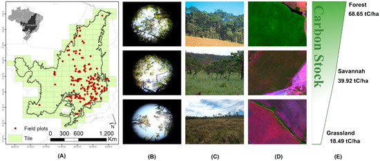
Figure 1.
(A) Location of the Cerrado biome in Brazil and its subdivision into tiles of 1.5 degree by 1.0 degree, and field plots (in red), which were used to explore the spectral differences between vegetation types; (B) “fisheye” field photographs showing the canopy cover in a forest (top), savanna (middle), and grassland (bottom); (C) panoramic field photos of forest, savanna, and grassland; (D) R5G4B3 representative Landsat-8 color composites of forest, savanna, and grassland; and (E) average carbon stock estimates in each vegetation [29].
The Cerrado has three predominant NV types, which can be classified according to their degree of woodiness, from grasslands to savanna woodlands and forests. According to the classification system proposed by Ribeiro and Walter [7], grasslands can be classified into two types: campo limpo and campo sujo, characterized by the predominance of herbaceous-shrub species and, to a lesser extent, sparsely distributed small trees. Savanna vegetation has a variable tree-shrub stratum, with a canopy cover ranging from 50% to 90%, which allows the coexistence of a grass layer. Forests (forested savannas, also known as cerradão, and riparian forests) present dense vegetation, with relatively large trees and low cover of grasses. Total plant biomass and carbon stocks in the Cerrado vary according to the type of vegetation, with an average of 18.5 t C ha−1 in grasslands, 39.9 t C ha−1 in savannas, and 68.6 t C ha−1 in forests [29]. Data on biomass and vegetation structure from 262 field inventory plots in the Cerrado compiled by Roitman et al. [38] were used to assess the spectral metrics that defined the different NV types, as detailed in the next session. The biome was partitioned in a regular grid of tiles compatible with the 1:250,000 international cartographic charts, where individual classifications were run for each tile. Each tile covers an area of 1° of latitude by 1° 30’ of longitude [30], generating a total of 172 tiles.
2.2. Classification Approach
The procedure to generate multi-temporal land cover maps in the Cerrado and to detect changes over time in the NV followed three main steps. The first step was the production of the year-based Landsat mosaics for the entire biome by defining the boundaries between the dry and wet seasons (Figure 2). These mosaics were used to generate spectral metrics, including sub-pixel fractions, indexes, and individual spectral bands. The second step included the selection of the best spectral variables for the definition of a preliminary empirical decision tree (EDT) classification, which in turn was used to derive a greater feature space to train the statistical decision tree (SDT) classifier. The last step was the classification of the annual mosaics using a machine learning approach, based on the class consistency map derived from the previous step.
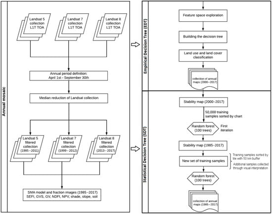
Figure 2.
Workflow of the procedures conducted to map annual native vegetation cover in the Brazilian Cerrado biome, including the production of the annual mosaics, the definition of the empirical decision tree classification, and the statistical decision tree classification. L1T TOA = Collection 1, Tier 1 top-of-atmosphere reflectance; SMA = spectral mixing analysis; SEFI = savanna ecosystem fraction index; GVS = green vegetation and shade; GV = green vegetation; NDFI = normalized difference fraction index; and NPV = non-photosynthetic vegetation.
2.2.1. Annual Landsat Mosaics
The historical changes from 1985 to 2017 in the Cerrado NV were mapped based on the Landsat-5 Thematic Mapper (TM), Landsat-7 Enhanced Thematic Mapper Plus (ETM+), and Landsat-8 Operational Land Imager (OLI). The Landsat top-of-atmosphere reflectance collection (Collection 1 Tier 1 TOA reflectance), with a 30 m spatial resolution, was accessed via Google Earth Engine (GEE) platform. The entire image processing procedure was also conducted in this platform for cloud removal, classification, and post-classification routines (links to the scripts available in the Supplementary Materials—Table S2).
For each tile, best-pixel annual mosaics were produced using a combination of pixels from distinct Landsat scenes gathered during the year in consideration. The temporal window defining the seasonal limits was evaluated at the state level because of the high variations in annual precipitation over the extent of the Cerrado. On the basis of the annual precipitation patterns for each state, we identified the optimum period (OP) of images to compose the annual mosaics, by integrating the six months from the end of the rainy season to the end of the dry season for each tile (Figure S1). This procedure aimed to reduce NV commission errors provided by a greener mosaic (for example, by considering images from the end of the rainy season), or NV omission errors by considering a drier mosaic, composed by images from the end of the dry season (July to September).
After the definition of the initial and final dates of the optimum period of the mosaic, a cloud and cloud shadow masking procedure, as well as a data dimensionality reduction based on pixel median, were conducted. The cloud and cloud shadow pixels were removed by a mask that was produced with the temporal dark outlier mask (TDOM) (see details of the TDOM in [39]) and complemented using the quality assessment bitmask (BQA) (see details in https://www.usgs.gov/land-resources/nli/landsat/landsat-collection-1-level-1-quality-assessment-band). The median algorithm was applied in each of the original bands, resulting in one final value per pixel and spectral band. The aggregation of this pixel-based composition of the annual mosaics was used for classification. To better represent seasonality, we used all normalized difference vegetation index (NDVI) values of the pixel in each year to produce dry and rainy median bands. The year-based NDVI values of each pixel were divided into quarters and the median pixels of the quarter with high NDVI were considered the rainy image and the median of the quarter with lower NDVI were considered the dry image.
2.2.2. Empirical Decision Tree
In order to derive a greater feature space used to train the statistical decision tree (SDT) classifier, an empirical decision tree was built with the most relevant parameters as inferred by the statistical evaluation of the input variables. This empirical decision tree (EDT) covered the period of 2000–2016, and sought to identify areas classified as the same NV over the entire period (stable samples). The factors selected for the EDT included the median of the original Landsat bands; spectral vegetation indices; and vegetation, non-photosynthetic vegetation, soil, and shade fractions derived from these bands (Table 1). A layer of slope data from the ALOS (Advanced Land Observing Satellite) global digital surface model with a 30 m resolution was also included (https://www.eorc.jaxa.jp/ALOS/en/aw3d30/index.htm).

Table 1.
List of predictive input spectral variables considered to be included in the empirical decision tree classification. The median statistics were applied to all variables. L5 = Landsat-5; L7 = Landsat-7; L8 = Landsat-8; Cloud = fractional abundance of cloud within the pixel; OP = optimum period.
This evaluation was conducted according to our feature space, which consisted of a sample of pixels selected based on 262 field inventory plots of the three NV types (see Figure 1 for the location of the plots within the biome) as well as samples from pasture and agriculture fields based on visual inspection. This procedure sought to identify the best metrics for highlighting the differences between NV types and major land-use classes such as pasture and agriculture fields (Figure S2). Among the metrics considered, those with the highest performances were the green vegetation (GV) index, non-photosynthetic vegetation (NPV) index, and soil and shade fractions, in addition to the green vegetation and shade (GVS) index and the savanna ecosystem fraction index (SEFI). While GVS highlights the difference between roughness and greenness of the vegetation, captured as the shade formed by the tree canopy [40], SEFI represents the combination of the amount of shade provided by the green vegetation with the non-photosynthetic materials and soils. Both GVS and SEFI were essential for separating forests and savannas from grasslands and other land use classes (pasture and agriculture) owing to the combination of vegetation heterogeneity and roughness, the amount of green material, and bare soil. Except for SEFI, which was developed for this study as an adaptation of the normalized difference fraction index (NDFI), the sub-pixel fraction images were based on the sub-pixel modeling and spectral library by Souza Jr. et al. [40].
Once the main input variables were selected, an EDT classification was semi-automatically created and calibrated with the variables for each tile and each year. A total of 2924 tiles (172 × 17 years) were calibrated based on the standard deviation values of each variable for each node, and manually adjusted using visual interpretation whenever necessary. The EDT is a conditional control statement algorithm used to support multistage decisions as a tree-like model consisting of a root node, several interior nodes, and several terminal nodes [42,43]. We used Fmask [45] as the first EDT node, which is a routine developed within the GEE platform to separate clouds, cloud shadow, and snow. Higher values of Fmask tend to be cloud and cloud shade, which, in this classification, were classified as non-observed areas. Non-observed areas on flat terrain were classified as water. Once the non-observed areas and water were classified, the remaining pixels were classified based on the V1 node defined by the SEFI variable. The combination of these fractions was used to distinguish the denser vegetation types from the sparser ones, capturing the differences between forests, savannas, and grasslands (Figure 3).
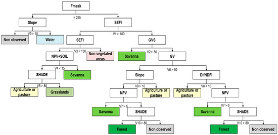
Figure 3.
Empirical decision tree classification scheme based on the values of the spectral metrics in 262 known field inventory plots in the Cerrado biome, seeking to separate native vegetation classes (grassland, savanna, and forest) from land use-related classes (mostly agriculture and pastures) and other non-vegetated areas (e.g., urban areas, bare soils). Values below each split refer to the factors at each node above it.
The V1 node represented the main node of the EDT classification scheme, where areas with medium and high SEFI values were classified as forest or savanna with higher tree density. In the upper branch of this node, the GVS index (V2 node) was used to define the first separation of the savanna from other classes. This node is followed by the GV index (V6 node), which aimed to separate young crops, dense forests, and savannas, with higher levels of GV and GVS, from sparser forests and savannas, and drier, more mature crops. In these last two branches, NPV (V7 node) was used to separate savanna from forest, as the former has a higher content of non-photosynthetic material than the latter. Finally, shade (V10 node) was used to distinguish areas classified as forest, but that were, in fact, non-observed areas shaded by topography. The lower branch of the tree is related to areas with a more open vegetation structure. Therefore, nodes V3, V4, and V5 were used to separate open savanna vegetation types from grasslands, and grasslands from pasture and agriculture fields. This branch (specifically, node V3) also included the definition of non-vegetated areas (e.g., urban areas, bare soil). The main variables used to define the nodes in this last branch were the combination of NPV and soil, and the amount of shade, which represents the heterogeneity of surface cover.
Given the lack of robust temporal datasets of land cover maps for the entire Cerrado to be used as reference for machine learning classification (MLC), we used the resulting annual land cover maps from the EDT classification from 2000 to 2016 (Mapbiomas Collection 2.0 classification of Cerrado biome with distinct vegetation types, available in https://mapbiomas.org) as a reference for the distribution of the random training samples for the MLC. This land cover database also used the TerraClass LULC map for 2013 [12] as the reference for the spatial distribution of the three main native vegetation types.
2.2.3. Statistical Decision Tree Classification
On the basis of the time series maps produced with the preliminary EDT classification, frequency maps were built to demonstrate the spatial and temporal consistency of each class, indicating the number of times in which each pixel was consistently classified as a given class throughout the period from 2000 to 2016. This routine created a map with frequency values ranging from 0 to 17, which is the total number of years in that period. The resulting values of this procedure ended up representing the probability of each pixel belonging to a given class. This probability map was used as the reference map to collect training samples for the SDT routines.
The application of the SDT to map NV types over 33 years was based on a machine learning approach with two main steps. In the first step, a new reference dataset of annual maps was created for an updated period from 2000 to 2017 (MapBiomas Collection 2.3, available in https://mapbiomas.org). In this initial SDT classification, the random forest classification algorithm (Breiman, 2001) available in the GEE platform was trained using 50,000 samples (pixels) per tile selected randomly in the areas mapped with higher frequency/consistency for each one of the three main NV types. The minimum number of years in which a pixel would have to be classified to consider a given class as consistent varied between classes (Table 2). The final number of training samples, therefore, varied between tiles as a function of the consistent area availability. Each combination of tile and year had its training sample dataset for application in the random forest classification round (number of trees = 100). The results of this classification were visually assessed to identify areas of spatial inconsistency between adjacent tiles. Additional training samples were included from neighboring tiles to increase consistency in areas of spatial discontinuity.
Table 2.
Probability thresholds were used to define areas of consistent classification for each land use and land cover (LULC) class. Values inside parentheses indicate the minimum number of years a pixel had to be classified as a given class to be considered consistent, considering a total of 17 years for the initial classification from 2000 to 2016, and 33 years for the final classification from 1985 to 2017. NA = not applicable. SDT, statistical decision tree.
In the second step, the NV maps resulting from the first random forest classification model were used to produce a new map of consistently classified NV classes. Over this map, new sampling points were selected to train the final map classification for the entire period (1985–2017) (MapBiomas Collection 3.1, available in https://mapbiomas.org). To address the issue of the spatial discontinuity between adjacent tiles in this final classification, the automatic sampling of points considered a buffer of 50 km around each tile. Such a procedure ensures that part of the training samples (about 10%) was representative of the variation found in the contact zone between tiles. Finally, additional samples were selected visually over the annual mosaics to complement the training samples in tiles with few consistently classified NV classes. The STD classifications were based on a larger number of spectral metrics including the ones extracted from the optimum mosaic and used for the EDT (Table 1), as well as other metrics retrieved for the entire annual dataset collection (Table S3).
2.3. Post Classification
A series of spatial and temporal filters were applied to the resulting maps in the GEE platform. The spatial filter segmented and indexed the classes of each collection into contiguous regions, which were subsequently identified and reclassified based on the following criterion: areas less than or equal to 0.5 ha (i.e., approximately 5 pixels) are reclassified based on the majority of the neighboring classes. A temporal filter was applied to identify and correct class transitions throughout the time series (i.e., 3 to 5 consecutive years), as well as to classify pixels with no data caused by cloud cover. For example, a pixel classified as non-forest in a given year ti (where i = 1985–2017), and forest in year ti − 1 and ti + 1, was reclassified as forest for the year ti. Several transition rules were defined and applied to be used in the temporal filter to deal with specific phenological and land use transitions (Table S4).
2.4. Integration with MapBiomas Cross-Cutting Themes
In order to implement the final MapBiomas land use and land cover maps for the Cerrado biome, the results of the Cerrado NV classification were integrated with other MapBiomas cross-cutting theme maps (e.g., pasture, agriculture, coastal zone, and urban infrastructure classes), which were independently developed [41,45]. This integration is hierarchical and follows prevalence rules to combine the classification results from all themes. For instance, urban areas and agriculture (i.e., crop fields) had prevalence over NV classes. More details are described in the ATBD (algorithm theoretical basis document) available at the MapBiomas website (http://mapbiomas.org/). After integration, the last step is spatial filtering to remove isolated class patches smaller than half a hectare as well as to remove noise caused by Landsat data misregistration. This spatial filter procedure is the same as described above in Section 2.3.
2.5. Accuracy Assessment
To assess the accuracy of each year and the NV classes, we used a set of 21,000 independent sampling points based on visual interpretation of Landsat data by three expert analysts (Figure S3). The sampling design and visual interpretation were performed by collaborators at the Image Processing and Geoprocessing Laboratory at the Federal University of Goiás, Brazil (LAPIG/UFG), using in the Temporal Visual Inspection web platform (tvi.lapig.iesa.ufg.br) [46]. The number of pixels collected to compose the reference dataset was pre-determined by statistical sampling techniques considering four tiles of the Cerrado subdivision (described in Section 2.1) as a minimum unit of analysis as well as six classes of slope, according to the shuttle radar topography mission data. The accuracy analysis was based on the approach proposed by Stehman et al. [47], using confusion matrix, overall accuracy, and omission and commission errors. The evaluation of a pixel in a given year was considered valid only when two or three interpreters agreed on the class observed in that pixel. The accuracy was then calculated using metrics that compare the class mapped with the class observed by the interpreters following the good practices proposed by Olofsson et al. [48]. We report year-based accuracy estimates with circa 5% error for each class in the mapping. The accuracy was reported for two levels of disaggregation: Level 1, which encompasses all three vegetation types as one class (NV); and Level 2, which separates all three types of NV.
2.6. Native Vegetation Net Loss
Once the annual NV maps were spatially and temporally filtered, NV net loss was calculated. The concept of NV net loss considered in this paper comprised the difference between the first and the last NV maps of the time series, representing the area difference of the Cerrado vegetation types in 1985 in comparison with 2017. Owing to the characteristics of the annual NV maps, which were built independently for each year, the net loss represented land cover change undergone by the NV over the past 33 years, accommodating both gains and losses over the whole time series.
2.7. Stability of Native Vegetation
The stability of the Cerrado NV was defined as the number of times in which a pixel was classified as the same given class (NV and non-NV) in the 17-year period initial SDT classification and in the 33-year period final SDT classification, indicating class consistency over time. The individual annual land cover maps were reclassified into four classes (forest; savanna; grassland; and non-NV land cover classes—agriculture, pasture, water, and non-vegetated areas). Next, they were overlaid and reduced to a single map to build this class consistency map. The NV stability map was classified into four classes for the final SDT classification (1985–2017): (i) stable NV areas classified as the same NV type in the 33 years of analysis; (ii) unstable NV areas, which had been classified as more than one vegetation type over time; (iii) stable non-NV areas, which had never been classified as NV over the time series; and (iv) NV areas converted to other non-NV land cover classes at some point in the time series, regardless of whether they subsequently recovered or not. The stability map was overlaid with the 2017 NV map indicating the current stable and unstable NV areas as well as the NV areas under recovery. The unstable NV areas and the NV areas converted to other land cover classes indicate natural and anthropogenic instability in the biome over the past three decades, respectively.
3. Results
3.1. Accuracy of Native Cerrado Vegetation Mapping
The strategy of using the semi-automatic calibrated EDT to retrieve the first set of annual consistent NV maps from 2000 to 2016 was fundamental for the improved performance of SDT classification. It guided the application of the SDT for the entire time series (1985 to 2017) in the highly complex Cerrado landscape, which lacked reference maps for gathering sets of training sampling points. The machine learning approach used here, which combined the SDT based on randomly selected samples in areas previously classified by the EDT as stable over the first time series (2000–2016), increased accuracy at Level 1 (where all NV types were aggregated as one NV class) by 4%: accuracy at Level 1 for the EDT alone was 83%, while accuracy for the final SDT classification (built upon the EDT-derived samples) was 87%.
The average overall accuracy of the final SDT classification at Level 2, analyzing the three NV classes separately, averaged 71%, ranging from 67% to 74% over the 33 years. The average balanced accuracy of forest (84%) was consistently higher than the accuracy of savanna (73%) and grassland (73%) throughout the time series (Figure S4). A confusion matrix was produced by aggregating the 33 annual confusion matrices into a single, average matrix (presented in Table S5). Also, omission and commission errors for all three classes throughout the time series are presented in Table S6. All classes presented high commission errors, with higher errors in the grasslands (Tables S5 and S6). These results suggest a relatively high degree of confusion between savanna and forests, and between savanna and grasslands, as expected in the naturally heterogeneous Cerrado. This is especially the case of cerradão, which, even in the field, can be alternately classified as a dense typical savanna or sparse forest. Confusion was higher with grasslands. Although the accuracy decreased from Level 1 to Level 2, as expected, it increased from the beginning to the end of the time series, and from the first to the final classifications.
3.2. Spatial and Temporal Patterns of the Cerrado Native Vegetation
The time series maps resulting from the SDT machine learning classification using the random forest algorithm indicated that, in 2017, 112 million hectares (Mha) (55%) of the original Cerrado range was still covered by native vegetation (Table 3). Among the three NV types, savanna is the most abundant. This class covered 52% (52.5 Mha) of the NV area in the biome in 2017 (i.e., 26% of the total area of the biome), followed by forest and grassland covering 36% (37.9 Mha) and 22% (22.2 Mha) of the total Cerrado NV, respectively (18% and 11% of the total area of the biome, respectively). Between 1985 and 2017, the Cerrado faced an overall net loss of 24.7 Mha, representing 10% of the original Cerrado distribution and 18% of the existing NV in 1985, resulting in 55% of the original NV distribution. Forests faced a net loss of almost half the total NV loss in the period, with 75% of this loss happening from 1985 to 2000. For savannas, a net loss of approximately 11 Mha could be observed, but, in contrast with the forests, the largest proportion of the net loss in the savanna happened after the year 2000 (52%) (Figure 4). Grasslands remained practically stable throughout this period, with an observed net loss of 1.9 Mha, representing 1% of the original range of the biome (Figure 5).
Table 3.
Native vegetation area in the Brazilian Cerrado at the beginning (1985) and the end (2017) of the time series, and net loss of native vegetation over the whole period between 1985 and 2017. Absolute and proportional net loss rates per year were also calculated. NV = native Cerrado vegetation.
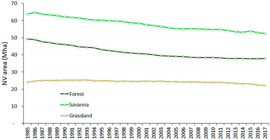
Figure 4.
Area (hectare) occupied by the three native vegetation types (forest in dark green, savanna in light green, and grassland in beige) in the Brazilian Cerrado over the time period of 1985–2017. Mha = million hectares; NV = native Cerrado vegetation.
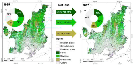
Figure 5.
Comparison between the first (1985) and last (2017) maps of the time series, showing the net loss of the three predominant native vegetation classes in relation to the total area of the Brazilian Cerrado. Mha = million hectares.
In the past 33 years (1985 to 2017), the native vegetation in the Cerrado biome has been declining at an average rate of 0.5% year (748,687 ha yr−1), particularly affecting forests and savannas (Figure 5, Table 3). Although savannas and forests presented similar amounts of area converted to other land use classes (around 11.3 million hectares), proportionally, forests lost more NV area than savannas (23% of forest loss in relation to 18% of savanna loss by 2017). Moreover, the forests presented a higher conversion rate from 1985 to 2017 (0.7% yr−1) compared with savannas (0.5% yr−1) and grasslands (0.2% yr−1), as the original area of forest is almost one-fourth of the original area of savanna (Table 3).
The remnant NV is located mostly in the center and northwestern part of the biome, more specifically in Mato Grosso (19%), Tocantins (18%), Maranhão (15%), Minas Gerais (18%), and Goiás (12%) (Table S7; Figure S6). These states account for almost 80% of the remaining Cerrado NV in 2017. Other states such as Bahia, Mato Grosso do Sul, and Piauí accounted for 19% of the current NV area in the biome (Table S7). Mato Grosso was the state that presented the highest levels of NV lost in the past 33 years, accounting for one-fourth of the whole NV net loss in the Cerrado from 1985 to 2017 (this state contains approximately 17% of the Cerrado area). The NV type lost that lost the most in this period in the Mato Grosso was savanna, followed by forest (Figure S7). Other states with important net loss of NV were Goiás and Mato Grosso do Sul (17% each), followed by Tocantins (13%), Maranhão (10%), Minas Gerais (8%), Bahia (7%), and Piauí (2%) (Table S7). Most of the NV net loss in Mato Grosso occurred between 1995 and 2005 (Figure S8), a period with large scale expansion of soybean in this state [49]. Mato Grosso do Sul and Goiás faced considerable losses in the 1985–1995 time period, being considered older agriculture frontier. The most recent NV net loss is happening in the states of the Matopiba region (Maranhão, Tocantins, Piauí, and Bahia). These four states together represent 55% of the loss of NV that happened recently from 2005 to 2017, representing the new region of Cerrado where agriculture is growing at the expense of NV loss [11,50].
Only 14% of the remaining Cerrado NV is protected in indigenous lands and conservation units. Grasslands are the most protected NV types (22% of their total area), followed by forests (17%) and savannas (9%) (Table S8). In the states where the majority of the NV conversion has already taken place, the remnant NV is mostly located within protected areas (states of São Paulo, Mato Grosso do Sul, and Mato Grosso) (Figure 5).
The distribution of the three NV classes and their net losses also varied depending on the regions of the Cerrado (Figure 6). Forests are dominant in the transition of the Cerrado to the Amazon biome, for example, in the northwestern portion of the states of Maranhão and western Mato Grosso. These two areas concentrated the largest NV losses. Savannas are currently concentrated mainly in the northeast of the biome (states of Tocantins, Bahia, and Piauí). The states of Mato Grosso, Mato Grosso do Sul, and Goiás presented the largest savanna losses along the time series. Grasslands are mainly clustered in the state of Tocantins and surrounding areas. Only a few tiles presented more than 50% of grassland loss over time.
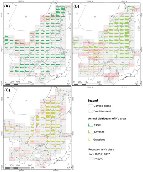
Figure 6.
Temporal distribution of (A) forest, (B) savanna, and (C) grassland per year and per tile from 1985 to 2017 in the Brazilian Cerrado. Tiles with a reduction of over 50% in each NV class over the time series are highlighted in red.
3.3. Stability of the Cerrado NV Classes
Forests were the vegetation type that presented the highest intra-annual map consistency, mostly concentrated in the northern portion of Maranhão state and western portion of Mato Grosso along the border with the Amazon biome (Figure 7; Table 4). Approximately 43% of NV areas mapped as forest from 1985 to 2017 were consistently mapped as forest from 27 to 33 times. Savanna was the second NV class in terms of temporal consistency, with 36% mapped consistently for more than 27 years over the biome. Concentration of savanna is found especially in Bahia and Piauí states. For grasslands, consistently mapped areas comprised 32% of the total grassland mapped, especially located in Tocantins and in the bordering Mato Grosso and Bahia states. Stable areas are primarily located in large fragments of NV (Figure 7 and Figure 8).
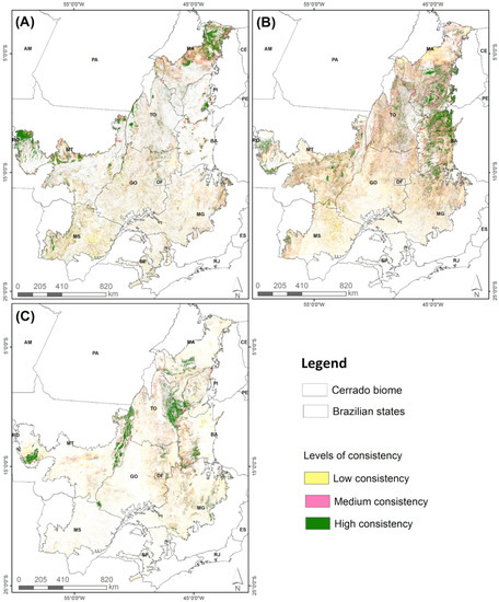
Figure 7.
Classification probability maps of three native vegetation classes (A—forest, B—savanna, and C—grassland) in the Brazilian Cerrado, indicating the levels of consistency (low: 1–11 years; medium: 12–26 years; and high: 27–33 years) observed for each class in the 1985–2017 period.
Table 4.
Consistency of the native vegetation classes in terms of the number of years in which the pixels were classified as the same class. Three consistency categories were considered: low: 1–11 years; medium: 12–26 years; and high: 27–33 years.
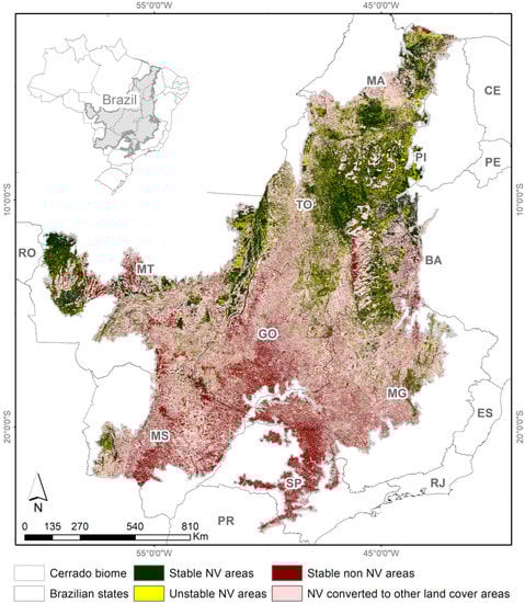
Figure 8.
Analysis of stability of native vegetation (NV) and other non-NV classes in the Brazilian Cerrado from 1985 to 2017, presenting stable NV and non-NV areas, as well as the unstable areas that either changed to other NV classes or to other non-NV land cover classes.
The stability map of the final SDT classification indicated that 36% of the Cerrado is composed of stable NV (classified as the same NV class over the entire time series) (Figure 8). Unstable areas of NV, which varied among different types of NV class, occupy 7% of the biome. Meanwhile, 38% of the biome was covered by NV that was converted to other land cover classes (e.g., pasture and crop fields), and 19% of areas that were classified as non-NV throughout the time series. These results suggest that the majority of the standing vegetation in 2017 is stable in terms of NV type (65%), while 12% varied among NV classes (natural instability) and 23% was converted at some point in time to other non-NV classes and recovered to NV by the end of the period (anthropogenic instability; Table 5).
Table 5.
Out of the area classified as native vegetation (NV) in 2017, the total area that did not change class (stable), the total area that changed among other NV classes (natural instability), and the total area that had been previously converted (anthropogenic instability followed by NV recovery).
4. Discussion
4.1. Innovative Machine Learning Approach to Map Temporal Dynamics of Cerrado Native Vegetation
The combination of a priori EDT with STD classification was able to adequately discriminate the three main NV types from a heterogeneous and seasonal biome, which is the case of the Brazilian Cerrado, over the entire time series of the Landsat mission (1985–2017). The use of cloud computing and the GEE platform has allowed the generation and calibration of automatic or semi-automatic methods for continuously monitoring land use and land cover with a medium to high spatial and temporal resolution over decades [51,52]. This procedure is a milestone in terms of creating robust baseline reference maps that can be used to train machine learning algorithms for monitoring and detecting changes in NV classes in complex and highly seasonal landscapes. This is especially relevant in regions where reference maps for guiding times series classification are insufficient or completely lacking. This is especially important for savanna ecosystems such as the Cerrado, which are currently undergoing changes owing to severe pressure for conversion, as well as facing degradation related to climate change [6,10,11].
Even though the Landsat image collection does not represent the most adequate imagery for capturing intra-annual or phenological variability of the NV because of the 16-day interval of image acquisition, it has been commonly used to map changes in NV in highly complex and variable ecosystems [22,26,53]. In addition, the Landsat mission is the only one that currently provides a historical perspective of change within a period of at least three decades of imagery with medium to high spatial resolutions [31,32]. It can also provide a consistent measure of the inter-annual variability of NV over the entire Earth’s surface. Some other initiatives have generated classification maps for the entire Brazilian Cerrado biome using Landsat free-archives (Table S1). The most widely used approaches in Brazil are the visual interpretation and traditional supervised classifications. These processes are very slow and costly, and classification is possible only in specific time periods [6,12,29,30] and was never applied to the entire Landsat series. Therefore, the generation of a semi-automatic method applied to long time series to discriminate the main types of NV present in the Cerrado biome with levels of accuracy compatible with existing initiatives was innovative and our main goal.
The results of this effort offer, to the scientific community, the first long-term annual dataset of NV (forest, savanna, and grassland) compatible with some of the few existing single-year NV maps for the biome. The average overall accuracy at Level 1 of 87% from 1985 to 2017 was similar to that obtained by Sano et al. [15] in their land cover map of the Cerrado for 2002 (90% overall accuracy), and by the TerraClass Cerrado Initiative for 2013 (80% overall accuracy). The distinction between NV classes from other land use types (Level 1 aggregation) presented an overall accuracy of 71%, which was the same as that reported by Sano et al. [15] (71% overall accuracy), but using much fewer points (315 field data validation points compared with 21,062 validation points used in this study) and only for a single year (2002). The accuracy increased from the beginning to the end of the time series, representing a gain of stability when we have a greater quality and quantity of images available.
The main challenges in distinguishing NV classes in the Cerrado include the misclassification between grasslands and planted pasture (ca. 8%), as well as the confusion between savannas and the other two NV types (forest and grasslands) [15]. Savannas are often misclassified as forests (omission error, ca. 39%), and grasslands are misclassified as savannas (commission error; ca. 46%) (Table S5). About 20% of pixels classified as forest were, in fact, savanna, while approximately 75% of the pixels classified as forest in the reference data were correctly classified (Table S5). Even though we had considerable errors of omission and commission at the edge of the NV types, this long time series allowed us to identify those areas where the stable vegetation is concentrated, and those where confusion among vegetation types is expected. This contributed greatly to the definition of the more unstable areas in the biome, and highlights where the map can and must be improved.
Moreover, the confusion among NV types occurs because they are distributed along a natural gradient of vegetation structure, with the savannas ranging from dense to very sparse woodlands dominated by grasses [7]. The study conducted by Ribeiro and Walter [7], or even the system of classification of vegetation proposed by the Brazilian Institute of Geography and Statistics (IBGE), subdivided the Cerrado into at least seven more detailed vegetation types, known as phytophysiognomies. The classification of these phytophysiognomies, which are defined by specific ranges of vegetation structure, is even more challenging. One way to improve this classification is by adding structural characteristics to the spectral components of the NV, such as height. Some studies have demonstrated the ability of LiDAR (Light Detection and Ranging) technology to differentiate between Cerrado vegetation types [54,55]. However, this time series represents the best comprehensive temporal data set on NV distribution in Cerrado.
4.2. Temporal and Spatial Dynamics of the Cerrado Native Vegetation
Up until 2017, remnant NV covered about 55% of the Brazilian Cerrado, although it was very unevenly distributed over the biome. While NV comprises 90% in the northern part of the biome, only 15% is left in its southern portions. The area classified as NV in 2017 included some areas of secondary NV. Although the approach used in this study generates temporally independent annual land cover maps that do not differentiate primary NV areas from regenerating areas, this proportion of remnant NV (55%) is compatible with those found in other studies [6,12].
Savannas still represent the predominant NV type in the Cerrado, occupying 52% of the NV area in 2017. Forests and grasslands occupy 36% and 22%, respectively. The prevalence of savannas is consistent with the results obtained by other authors [6,12]. This distribution is explained by the spatial configuration of the Cerrado NV, forming a gradient of mosaics related to a series of continuous environmental characteristics such as topography, soil, and climate [7].
Over the last three decades, the annual net loss rate of the Cerrado NV was 0.50% per year or 748,687 ha per year, which is 20% lower than the official annual gross deforestation estimates for the past 10 years (944,521 ha yr−1) [12]. This difference was expected as our concept of NV net loss includes NV areas that recovered after conversion, while gross deforestation estimates by the National Institute of Spatial Research (INPE) [12] do not include them. Beuchle et al. [23] reported a 0.60% net loss rate from 2000 to 2010 for the Cerrado biome, which is comparable to our observed average rate. Most of the net loss occurring in the first half of the time series (1985 to 2000) was in forests owing to cropland expansion.
The majority of the NV net loss occurred in the southern part of the Cerrado, in the states of Goiás, Mato Grosso do Sul, and Mato Grosso (Table S7), and mainly in the early stages of the time series, so that they are considered as older frontiers of agricultural expansion in the country. In these regions, most of the remaining NV mapped in 2017 is located within protected areas. The newest agriculture frontier in the Cerrado, responsible for large-scale deforestation, is located in the northern part of Cerrado, in a region known as MATOPIBA (southern portion of states of Maranhão and Piauí, north of Tocantins and west of Bahia) [11,56]. Native vegetation conversion to agricultural areas in the Cerrado biome is related to biophysical characteristics and infrastructure improvements [57].
Savannas and forests were the most affected NV types in terms of net loss due to the increase of pastures and agriculture in the biome along with the time series. Even though savannas are the most abundant vegetation type in the biome, forests faced most of the net loss over the time series. While savannas lost 11 Mha in 33 years, forests accounted for a comparable net loss in absolute terms, even though they represent two-thirds of the area of savanna. Grasslands correspond to the areas mostly unsuitable for agriculture usually owing to them being located over shallow and poor soils, and despite being mostly unprotected by law [57]. Detecting conversion of grasslands was quite difficult because of the spectral confusion between native grasslands and planted pastures, usually requiring observations of phenological timings [26]. These timings are easily missed by monitoring approaches that do not capture intra-annual changes, which is corroborated by the lower accuracies observed for this class.
4.3. Stability of the Cerrado Native Vegetation Classes
In a highly seasonal and heterogeneous biome, vegetation stability evaluation is a challenge that can be overcome with consistent long-term information. We managed to identify areas where specific types of NV are dominant, as well as areas with high instability in terms of NV mapping. This strategy demonstrated that the forests presented the highest consistency over time compared with savannas and grasslands in the Brazilian Cerrado. On the other hand, grasslands were the NV with the lowest mapping consistency over time. These patterns are expected and can be explained by the effects of seasonality on the spectral response of NV types dominated by grasses, which are more susceptible to drought [15,20]. These results also help to guide further improvements in classifying the unstable NV areas using either higher temporal and/or spatial resolution imagery.
The consistency maps can be also used to suggest whether the main drivers of instability are either natural (e.g., seasonality, fire) or anthropogenic (e.g., NV conversion to agriculture). In this way, we identified that 36% of the Cerrado is covered by NV that was mapped consistently over time as a specific NV class, so it can be considered as stable. Only 7% of the biome presented NV classes that were highly unstable in terms of mapping, probably associated with natural disturbances. Other areas of high NV instability were related to areas that, at some point in time, were converted to other land uses (e.g., agriculture and pasture), representing 38% of the biome, and were considered anthropogenic. This analysis suggests that, from 55% of the Cerrado area with NV, only 43% remained as NV during at least 33 years. When the stability map was masked by the 2017 NV map, it revealed that the majority (62%) of the NV types were stable over time, while 23% were in the process of recovery. This indicates that around 12% of the Cerrado biome is currently in the process of regeneration. These numbers are fundamental for assisting public policies towards Cerrado conservation.
5. Conclusions
This study was the first to apply a combination of EDT and SDT classification techniques for mapping different types of native vegetation in the Cerrado biome, using a long time series of satellite data (1985–2017). The use of Landsat archive and cloud computing freely available in the Google Earth Engine platform allowed the generation and calibration of a semi-automatic method for monitoring the spatiotemporal land cover dynamics over three decades. We managed to obtain annual-based estimates of the remnant NV in this biome dominated by a very heterogeneous landscape, marked seasonality, and intensive human land occupation. The results showed that approximately 45% of the Cerrado NV was converted into some type of land use and land occupation by 2017. The conversion is occurring rapidly, especially in the northern part of the biome where most of the remnant NV is found nowadays. This study also showed some areas where the NV appeared as a mosaic of grasslands, savannas, and forests, indicating a limitation of Landsat data to discriminate these three vegetation types properly, perhaps because of its moderate spatial resolution (30 m). Despite our promising results, discriminating different NV types in highly seasonal and heterogeneous ecosystems such as the Cerrado remains challenging, especially if the goal is to discriminate between phytophysiognomies rather than general classes. As a future investigation, we suggest including other satellite data such as the Sentinel-1 (radar) and Sentinel-2 (optical) images obtained with 10 m spatial resolution and repeat pass of five days, which are available on the Internet without cost.
Supplementary Materials
The following supplementary materials are available online at https://www.mdpi.com/2072-4292/12/6/924/s1, Table S1. Characteristics of the existing native vegetation maps covering the entire Brazilian Cerrado and produced by semi-automatic methods and visual interpretation of varying remote sensing data; Table S2. Scripts used in the initial and final statistical decision tree classification of the native Cerrado vegetation; Table S3. Spectral metrics, indexes, and other variables used to train the random forest SDT classification; Table S4. Rules of the temporal filters applied to classify native Cerrado vegetation. RG = General Rule; RP = First Year Rule; RU = Last Year Rule; FF = Forest; SV = Savanna; GL = Grassland; AG = Mosaic of Agriculture and Pasture; AR = Rocky Outcrop; WB = Water; and NO = Non-Observed; Table S5. Confusion matrix of NV classes at level 2. Other land cover classes include agriculture and pasture fields and non-vegetated areas. UA = user´s accuracy; PA = producer’s accuracy; Table S6. Omission and commission errors of the 33 classified maps; Table S7. State-level distribution of native vegetation (NV) and NV net loss from 1985 to 2017; Table S8. Distribution of the native Cerrado vegetation (NV) inside protected areas (indigenous lands and conservation units) from 1985 to 2017; Figure S1. Mean monthly precipitation and normalized difference vegetation index (NDVI) data from forest and savanna vegetation. Gray rectangle corresponds to the six-month optimum period for deriving the Landsat mosaic of the Brazilian Cerrado; Figure S2. Boxplots representing the distribution of the dominant land cover classes of the Brazilian Cerrado over six spectral metrics included in the empirical decision tree classification. GVS = green vegetation and shade; GV = green vegetation; NPV = non-photosynthetic vegetation; SEFI = savanna ecosystem fraction index; Figure S3. Location of 21,000 sampling points used for accuracy assessment. Other = water, non-vegetated, agriculture, and pasture fields; Figure S4. Overall accuracy for the three classifications (empirical decision tree (EDT), initial statistical decision tree (SDT), and final SDT), considering the aggregated legend; Figure S5. State-level proportion of native vegetation (NV) in 2017, other non-NV land cover types in 2017, and NV net loss from 1985 to 2017. MS—Mato Grosso do Sul, GO—Goiás, MT—Mato Grosso, TO—Tocantins, MA—Maranhão, MG—Minas Gerais, BA—Bahia, PI—Piauí, SP—São Paulo, and DF—Federal District; Figure S6. State-level net loss of native vegetation (NV) from 1985 to 2017. Mha = million hectares. See Figure S6 for state identification; Figure S7. State-level native vegetation (NV) net loss in three different periods: 1985–1995, 1995–2005, and 2005–2017. M ha = million hectares. See Figure S6 for state identification.
Author Contributions
Conceptualization, A.A. and J.Z.S.; Methodology, A.A., M.R., F.L., C.B.M., and J.Z.S.; Validation, A.A., F.L., C.B.M., I.C., I.A., and J.Z.S.; Formal analysis, A.A., F.L., C.B.M., B.Z., I.C., V.A., and J.Z.S.; Investigation, A.A., F.L., C.B.M., V.A., J.P.F.M.R., J.Z.S., I.C., I.A., M.M.C.B., E.E.S., M.B., V.R., and V.P.; Writing—original draft preparation, A.A., J.Z.S., and B.Z.; Writing—review and editing, A.A., J.Z.S., F.L., B.Z., C.B.M., M.M.C.B., M.R., E.E.S., and M.B.; Visualization, A.A., B.Z., F.L., C.B.M., V.A., J.P.F., M.R., V.V., and I.C.; Supervision, A.A.; Project administration, A.A. and J.Z.S.; Funding acquisition, A.A., J.Z.S., and M.B. All authors have read and agreed with the published version of the manuscript.
Funding
This research was conducted by the MapBiomas Initiative. It was financed by the Moore Foundation, with the support of The Nature Conservancy, as well as the UK Space Agency’s International Partnership Programme (IPP) under the Global Challenge Research Fund (GCRF), with the support of Ecometrica.
Acknowledgments
The authors would like to thank the MapBiomas team and Google Earth Engine for providing access to the Landsat cloud processing. The authors are grateful for the field plot locations and accuracy analysis from University of Brasília and Federal University of Goiás/LAPIG, respectively.
Conflicts of Interest
The authors declare no conflict of interest. The funders had no role in the design of the study, in the collection, analysis, or interpretation; in the writing of the manuscript; or in the decision to publish the results.
References
- Bourlière, F.; Hadley, M. Present-day savannas: An overview. In Tropical Savannas; Bourlière, F., Ed.; Elsevier: Amsterdam, The Netherlands, 1983; pp. 1–17. [Google Scholar]
- Scholes, R.J.; Hall, D.O. The carbon budget of tropical savannas, woodlands and grasslands. Sci. Comm. Probl. Environ. Int. Counc. Sci. Unions 1996, 56, 69–100. [Google Scholar]
- Solbrig, O.T. The diversity of the savanna ecosystem. In Biodiversity and Savanna Ecosystem Processes; Springer: Berlin/Heidelberg, Germany, 1996; pp. 1–27. [Google Scholar]
- Gillson, L. Evidence of Hierarchical Patch Dynamics in an East African Savanna? Landsc. Ecol. 2004, 19, 883–894. [Google Scholar] [CrossRef]
- Marchant, R. Understanding complexity in savannas: Climate, biodiversity and people. Curr. Opin. Environ. Sustain. 2010, 2, 101–108. [Google Scholar] [CrossRef]
- Sano, E.E.; Rosa, R.; Scaramuzza, C.A.M.; Adami, M.; Bolfe, E.L.; Coutinho, A.C.; Esquerdo, J.C.D.M.; Maurano, L.E.P.; da Narvaes, I.S.; de Oliveira Filho, F.J.B.; et al. Land use dynamics in the Brazilian Cerrado in the period from 2002 to 2013. Pesqui. Agropecuária Bras. 2019, 54. [Google Scholar] [CrossRef]
- Ribeiro, J.F.; Walter, B.M.T. Fitofisionomia do Bioma Cerrado. In Cerrado: Ambiente e Flora; Sano, S.M., Almeida, S.P., Eds.; Embrapa: Brasilia, Brazil, 1998; pp. 89–166. [Google Scholar]
- Mittermeier, R.A.; Turner, W.R.; Larsen, F.W.; Brooks, T.M.; Gascon, C. Global Biodiversity Conservation: The Critical Role of Hotspots. In Biodiversity Hotspots; Springer: Berlin/Heidelberg, Germany, 2011; pp. 3–22. [Google Scholar]
- Strassburg, B.B.N.; Brooks, T.; Feltran-Barbieri, R.; Iribarrem, A.; Crouzeilles, R.; Loyola, R.; Latawiec, A.E.; Oliveira Filho, F.J.B.; Scaramuzza, C.A.M.; Scarano, F.R.; et al. Moment of truth for the Cerrado hotspot. Nat. Ecol. Evol. 2017, 1, 99. [Google Scholar] [CrossRef] [PubMed]
- Bustamante, M.; Nardoto, G.; Pinto, A.; Resende, J.; Takahashi, F.; Vieira, L. Potential impacts of climate change on biogeochemical functioning of Cerrado ecosystems. Braz. J. Biol. 2012, 72, 655–671. [Google Scholar] [CrossRef]
- Spera, S.A.; Galford, G.L.; Coe, M.T.; Macedo, M.N.; Mustard, J.F. Land-use change affects water recycling in Brazil’s last agricultural frontier. Glob. Chang. Biol. 2016, 22, 3405–3413. [Google Scholar] [CrossRef]
- INPE (Instituto Nacional de Pesquisas Espaciais). Programa de Monitoramento da Amazônia e Demais Biomas—Bioma Cerrado. Available online: http://terrabrasilis.dpi.inpe.br/downloads/ (accessed on 10 November 2018).
- Rocha, G.F.; Ferreira, L.G.; Ferreira, N.C.; Ferreira, M.E. Detecção de desmatamentos no bioma Cerrado entre 2002 e 2009: Padrões, tendências e impactos. Rev. Bras. Cart. 2011, 3, 341–349. [Google Scholar]
- Dias, L.C.P.; Macedo, M.N.; Costa, M.H.; Coe, M.T.; Neill, C. Effects of land cover change on evapotranspiration and streamflow of small catchments in the Upper Xingu River Basin, Central Brazil. J. Hydrol. Reg. Stud. 2015, 4, 108–122. [Google Scholar] [CrossRef]
- Sano, E.E.; Rosa, R.; Brito, J.L.S.; Ferreira, L.G. Land cover mapping of the tropical savanna region in Brazil. Environ. Monit. Assess. 2010, 166, 113–124. [Google Scholar] [CrossRef]
- Glenn, E.; Huete, A.; Nagler, P.; Nelson, S. Relationship Between Remotely-sensed Vegetation Indices, Canopy Attributes and Plant Physiological Processes: What Vegetation Indices Can and Cannot Tell Us about the Landscape. Sensors 2008, 8, 2136–2160. [Google Scholar] [CrossRef] [PubMed]
- Jacon, A.D.; Galvão, L.S.; dos Santos, J.R.; Sano, E.E. Seasonal characterization and discrimination of savannah physiognomies in Brazil using hyperspectral metrics from Hyperion/EO-1. Int. J. Remote Sens. 2017, 38, 4494–4516. [Google Scholar] [CrossRef]
- Roy, D.P.; Boschetti, L.; Giglio, L. Remote Sensing of Global Savana Fire Occurrence, Extent, and Properties. In Ecosystem Function in Savannas: Measurement and Modeling at Landscape to Global Scales; Hill, M.J., Hanan, N.P., Eds.; CRC Press: Boca Raton, FL, USA, 2011; pp. 239–254. [Google Scholar]
- Gomes, L.; Miranda, H.S.; Silvério, D.V.; Bustamante, M.M.C. Effects and behaviour of experimental fires in grasslands, savannas, and forests of the Brazilian Cerrado. For. Ecol. Manage. 2020, 458, 117804. [Google Scholar] [CrossRef]
- Ferreira, L.G.; Huete, A.R. Assessing the seasonal dynamics of the Brazilian Cerrado vegetation through the use of spectral vegetation indices. Int. J. Remote Sens. 2004, 25, 1837–1860. [Google Scholar] [CrossRef]
- Ratana, P.; Huete, A.R.; Ferreira, L. Analysis of Cerrado Physiognomies and Conversion in the MODIS Seasonal–Temporal Domain. Earth Interact. 2005, 9, 1–22. [Google Scholar] [CrossRef]
- Ferreira, M.E.; Ferreira, L.G.; Sano, E.E.; Shimabukuro, Y.E. Spectral linear mixture modelling approaches for land cover mapping of tropical savanna areas in Brazil. Int. J. Remote Sens. 2007, 28, 413–429. [Google Scholar] [CrossRef]
- Beuchle, R.; Grecchi, R.C.; Shimabukuro, Y.E.; Seliger, R.; Eva, H.D.; Sano, E.; Achard, F. Land cover changes in the Brazilian Cerrado and Caatinga biomes from 1990 to 2010 based on a systematic remote sensing sampling approach. Appl. Geogr. 2015, 58, 116–127. [Google Scholar] [CrossRef]
- Schwieder, M.; Leitão, P.J.; da Cunha Bustamante, M.M.; Ferreira, L.G.; Rabe, A.; Hostert, P. Mapping Brazilian savanna vegetation gradients with Landsat time series. Int. J. Appl. Earth Obs. Geoinf. 2016, 52, 361–370. [Google Scholar] [CrossRef]
- Hill, M.J.; Zhou, Q.; Sun, Q.; Schaaf, C.B.; Palace, M. Relationships between vegetation indices, fractional cover retrievals and the structure and composition of Brazilian Cerrado natural vegetation. Int. J. Remote Sens. 2017, 38, 874–905. [Google Scholar] [CrossRef]
- Müller, H.; Rufin, P.; Griffiths, P.; Barros Siqueira, A.J.; Hostert, P. Mining dense Landsat time series for separating cropland and pasture in a heterogeneous Brazilian savanna landscape. Remote Sens. Environ. 2015, 156, 490–499. [Google Scholar] [CrossRef]
- Brazil, M. TerraClass: Mapeamento do Uso e Cobertura do Cerrado: Projeto TerraClass Cerrado 2013; Ministério do Meio Ambiente (MMA): Brasilia, Brazil, 2015.
- Fbds, F.B.; Para, D.S. Projeto de Mapeamento em Alta Resolução dos Biomas Brasileiros. Available online: http://geo.fbds.org.br/ (accessed on 1 November 2019).
- Ministério da Ciência, Tecnologia e Inovação. III Inventário Brasileiro de Emissões e Remoções Antrópicas de Gases de Efeito Estufa não Controlados pelo Protocolo de Montreal; MCTIC: Brasilia, Brazil, 2015.
- IBGE. Monitoramento da Cobertura e uso da Terra—2000, 2010, 2012, 2014, 2015—Em Grade Territorial Estatística; IBGE: Rio de Janeiro, Brazil, 2017. [Google Scholar]
- Wulder, M.A.; White, J.C.; Loveland, T.R.; Woodcock, C.E.; Belward, A.S.; Cohen, W.B.; Fosnight, E.A.; Shaw, J.; Masek, J.G.; Roy, D.P. The global Landsat archive: Status, consolidation, and direction. Remote Sens. Environ. 2016, 185, 271–283. [Google Scholar] [CrossRef]
- Phiri, D.; Morgenroth, J. Developments in Landsat Land Cover Classification Methods: A Review. Remote Sens. 2017, 9, 967. [Google Scholar] [CrossRef]
- Gorelick, N.; Hancher, M.; Dixon, M.; Ilyushchenko, S.; Thau, D.; Moore, R. Google Earth Engine: Planetary-scale geospatial analysis for everyone. Remote Sens. Environ. 2017, 202, 18–27. [Google Scholar] [CrossRef]
- Parente, L.; Mesquita, V.; Miziara, F.; Baumann, L.; Ferreira, L. Assessing the pasturelands and livestock dynamics in Brazil, from 1985 to 2017: A novel approach based on high spatial resolution imagery and Google Earth Engine cloud computing. Remote Sens. Environ. 2019, 232, 111301. [Google Scholar] [CrossRef]
- IBGE. Biomas e Sistema Costeiro-Marinho do Brasil: Compatível com a Escala 1:250.000; IBGE: Rio de Janeiro, Brazil, 2019. [Google Scholar]
- Assad, E.D. Chuva nos Cerrados: Análise e Espacialização; Embrapa-CPAC: Brasilia, Brazil, 1994. [Google Scholar]
- Coutinho, L.M. O bioma do cerrado. In Eugen Warming e o Cerrado Brasileiro: Um Século Depois; UNESP: São Paulo, Brazil, 2002; pp. 77–91. [Google Scholar]
- Roitman, I.; Bustamante, M.M.C.; Haidar, R.F.; Shimbo, J.Z.; Abdala, G.C.; Eiten, G.; Fagg, C.W.; Felfili, M.C.; Felfili, J.M.; Jacobson, T.K.B.; et al. Optimizing biomass estimates of savanna woodland at different spatial scales in the Brazilian Cerrado: Re-evaluating allometric equations and environmental influences. PLoS ONE 2018, 13, e0196742. [Google Scholar] [CrossRef]
- Housman, I.; Chastain, R.; Finco, M. An Evaluation of Forest Health Insect and Disease Survey Data and Satellite-Based Remote Sensing Forest Change Detection Methods: Case Studies in the United States. Remote Sens. 2018, 10, 1184. [Google Scholar] [CrossRef]
- Souza, C.M.; Roberts, D.A.; Cochrane, M.A. Combining spectral and spatial information to map canopy damage from selective logging and forest fires. Remote Sens. Environ. 2005, 98, 329–343. [Google Scholar] [CrossRef]
- Diniz, C.; Cortinhas, L.; Nerino, G.; Rodrigues, J.; Sadeck, L.; Adami, M.; Souza-Filho, P. Brazilian Mangrove Status: Three Decades of Satellite Data Analysis. Remote Sens. 2019, 11, 808. [Google Scholar] [CrossRef]
- Swain, P.H.; Hauska, H. The decision tree classifier: Design and potential. IEEE Trans. Geosci. Electron. 1977, 15, 142–147. [Google Scholar] [CrossRef]
- Safavian, S.R.; Landgrebe, D. Separating and tracking multiple beacon sources for deep space optical communications. Free. Laser Commun. Technol. XXII 1991, 21, 660–674. [Google Scholar]
- Zhu, Z.; Woodcock, C.E. Continuous change detection and classification of land cover using all available Landsat data. Remote Sens. Environ. 2014, 144, 152–171. [Google Scholar] [CrossRef]
- Parente, L.; Ferreira, L. Assessing the Spatial and Occupation Dynamics of the Brazilian Pasturelands Based on the Automated Classification of MODIS Images from 2000 to 2016. Remote Sens. 2018, 10, 606. [Google Scholar] [CrossRef]
- Nogueira, S.H.M.; Parente, L.L.; Ferreira, L.G. Temporal Visual Inspection: Uma Ferramenta Destinada À Inspeção Visual De Pontos Em Séries Históricas De Imagens De Sensoriamento Remoto. In Proceedings of the Anais do XXVII Congresso Brasileiro de Cartografia e XXVI Exposicarta, Rio de Janeiro, Brazil, 6–9 November 2017; pp. 624–628. [Google Scholar]
- Stehman, S.V. Estimating area and map accuracy for stratified random sampling when the strata are different from the map classes. Int. J. Remote Sens. 2014, 35, 4923–4939. [Google Scholar] [CrossRef]
- Olofsson, P.; Foody, G.M.; Herold, M.; Stehman, S.V.; Woodcock, C.E.; Wulder, M.A. Good practices for estimating area and assessing accuracy of land change. Remote Sens. Environ. 2014, 148, 42–57. [Google Scholar] [CrossRef]
- Macedo, M.N.; DeFries, R.S.; Morton, D.C.; Stickler, C.M.; Galford, G.L.; Shimabukuro, Y.E. Decoupling of deforestation and soy production in the southern Amazon during the late 2000s. Proc. Natl. Acad. Sci. USA 2012, 109, 1341–1346. [Google Scholar] [CrossRef]
- Zalles, V.; Hansen, M.C.; Potapov, P.V.; Stehman, S.V.; Tyukavina, A.; Pickens, A.; Song, X.P.; Adusei, B.; Okpa, C.; Aguilar, R.; et al. Near doubling of Brazil’s intensive row crop area since 2000. Proc. Natl. Acad. Sci. USA 2019, 116, 428–435. [Google Scholar] [CrossRef]
- Azzari, G.; Lobell, D.B. Landsat-based classification in the cloud: An opportunity for a paradigm shift in land cover monitoring. Remote Sens. Environ. 2017, 202, 64–74. [Google Scholar] [CrossRef]
- Deines, J.M.; Kendall, A.D.; Crowley, M.A.; Rapp, J.; Cardille, J.A.; Hyndman, D.W. Mapping three decades of annual irrigation across the US High Plains Aquifer using Landsat and Google Earth Engine. Remote Sens. Environ. 2019, 233, 111400. [Google Scholar] [CrossRef]
- Grecchi, R.C.; Gwyn, Q.H.J.; Bénié, G.B.; Formaggio, A.R. Assessing the spatio-temporal rates and patterns of land-use and land-cover changes in the Cerrados of southeastern Mato Grosso, Brazil. Int. J. Remote Sens. 2013, 34, 5369–5392. [Google Scholar] [CrossRef]
- Ferreira, L.G.; Urban, T.J.; Neuenschawander, A.; de Araújo, F.M. Use of Orbital LIDAR in the Brazilian Cerrado Biome: Potential Applications and Data Availability. Remote Sens. 2011, 3, 2187–2206. [Google Scholar] [CrossRef]
- Zimbres, B.; Shimbo, J.; Bustamante, M.; Levick, S.; Miranda, S.; Roitman, I.; Silvério, D.; Gomes, L.; Fagg, C.; Alencar, A. Savanna vegetation structure in the Brazilian Cerrado allows for the accurate estimation of aboveground biomass using terrestrial laser scanning. For. Ecol. Manage. 2020, 458, 117798. [Google Scholar] [CrossRef]
- Noojipady, P.; Morton, C.D.; Macedo, N.M.; Victoria, C.D.; Huang, C.; Gibbs, K.H.; Bolfe, L.E. Forest carbon emissions from cropland expansion in the Brazilian Cerrado biome. Environ. Res. Lett. 2017, 12, 025004. [Google Scholar] [CrossRef]
- Garcia, A.S.; Ballester, M.V.R. Land cover and land use changes in a Brazilian Cerrado landscape: Drivers, processes, and patterns. J. Land Use Sci. 2016, 11, 538–559. [Google Scholar] [CrossRef]


© 2020 by the authors. Licensee MDPI, Basel, Switzerland. This article is an open access article distributed under the terms and conditions of the Creative Commons Attribution (CC BY) license (http://creativecommons.org/licenses/by/4.0/).