Abstract
We demonstrate precise determination of atmospheric temperature using vibro-rotational Raman (VRR) spectra of molecular nitrogen and oxygen in the range of 292–293 K. We used a continuous wave fiber laser operating at 10 W near 532 nm as an excitation source in conjunction with a multi-pass cell. First, we show that the approximation that nitrogen and oxygen molecules behave like rigid rotors leads to erroneous derivations of temperature values from VRR spectra. Then, we account for molecular non-rigidity and compare four different methods for the determination of air temperature. Each method requires no temperature calibration. The first method involves fitting the intensity of individual lines within the same branch to their respective transition energies. We also infer temperature by taking ratios of two isolated VRR lines; first from two lines of the same branch, and then one line from the S-branch and one from the O-branch. Finally, we take ratios of groups of lines. Comparing these methods, we found that a precision up to 0.1 K is possible. In the case of O, a comparison between the different methods show that the inferred temperature was self-consistent to within 1 K. The temperature inferred from N differed by as much as 3 K depending on which VRR branch was used. Here we discuss the advantages and disadvantages of each method. Our methods can be extended to the development of instrumentation capable of non-invasive monitoring of gas temperature with broad potential applications, for example, in laboratory, ground-based, or airborne remote sensing.
1. Introduction
Small changes in temperature can have non-linear effects on a number of processes. One such case is the nucleation of non-sea-salt sulfate particles from sulfuric acid in the atmosphere, where a decrease in temperature of a couple of degrees Celsius can result in an order of magnitude increase in new particle formation [1]. As a result, fluctuations in temperature can result in enhanced nucleation rates of particles. For example, Platis et. al. [2] observed a new particle formation event in an inversion layer with large fluctuations in temperature. However, often measurements of the inversion layer are limited by coarse time resolution, and the direct relation between temperature fluctuations and new particle formation is unknown. Also, fluctuations in water vapor saturation ratio are dependent on temperature fluctuations [3]. The conditions most favorable for new particle formation involving water are those where saturation ratio and temperature are anti-correlated [2,4]. Temperature fluctuations can also affect the supersaturation in clouds, which in turn determines the activation and eventual growth of cloud droplets. In fact, thermodynamic fluctuations due to turbulent mixing in clouds may broaden the size distribution of droplets, which has implications for precipitation and the cloud optical properties [5,6]. In order to understand the effect that temperature fluctuations can have on the evolution of aerosol and cloud droplets, continuous monitoring of temperature would be ideal. This can be difficult above the ground level using direct means of temperature measurements, which are often performed by aircraft and radiosondes. Temperature fluctuations can be difficult for aircraft to measure, especially in clouds where condensation can limit the time response and accuracy of temperature measurements [7]. While research aircraft are capable of high temporal and spatial resolution measurements in the horizontal direction (along the flight path), the range-resolved resolution of these measurements is poor [8]. Remote sensing techniques cannot just provide vertical profiles, but can also monitor the evolution of those vertical profiles over time.
Raman and Rayleigh scattering techniques are used in a variety of applications where temperature must be determined remotely [9]. Some of these techniques have been developed to measure the temperature during combustion processes, while others have been developed to measure atmospheric temperature. For example, Rayleigh scattering is often used to measure changes in molecular number density in flames which are in turn related to temperature using the ideal gas law under the assumption that the medium being measured has constant pressure and known molecular composition [10,11]. Additionally, changes in laser intensity, and elastic scattering from large particles, must be accounted for when using Rayleigh techniques; in fact, cloud droplets and dust, can degrade the precision of the technique [9]. In an alternative approach, the intensity of pure rotational Raman (PRR) transitions can be used to determine the temperature of flames and the atmosphere without needing to make assumptions about the pressure or the composition of the gas [12]. PRR light detection and ranging (LiDAR) is the most widely accepted remote air temperature measurement technique used by the atmospheric LiDAR community [13,14,15]. A significant advantage of Raman-based techniques is the ability to take a ratio of two portions of the scattered spectrum, eliminating the need to monitor the laser intensity. However, the close proximity of the rotational Raman lines to elastic scattering presents a significant challenge especially in turbid environments, such as clouds. Modern narrow band-pass filters have allowed the technique to be employed with minimal systematic errors in aerosol layers and optically thin clouds [16]. Several methods have been developed to extract temperature information from the vibrational spectra of N and O, which are spectrally separated from elastic scattering [17]. The spectral separation allows for the use of optical filters that attenuate elastically scattered light better to reduce the systematic errors imposed by large particle scattering. The Stoke’s vibrational line has also been used for satellite-based temperature determination in the stratosphere using a similar principle to the Rayleigh methods described above, but Rayleigh measurements are necessary to estimate density [18]. Temperature can also be determined by taking a ratio of the Stoke’s and anti-Stoke’s pure vibrational scattering; however this technique is not tenable at atmospherically relevant temperatures due to weak anti-Stoke’s signal [9]. Several hybrid methods have also been developed to estimate atmospheric temperature. Su et al. compared the Stoke’s Q-Branch Raman transition to a PRR line with a high rotational quantum number to determine atmospheric temperature up to a height of 22 km. The technique determined the temperature within a cloud to within 1.5 K of a radiosonde measurement [19].
Temperature can be determined from the vibro-rotational S- and O-branches of the vibro-rotational Raman (VRR) spectrum of O and N in a similar fashion to the PRR spectrum. For both cases, Maxwell-Boltzmann statistics dictates that molecules populating lower energy rotational states will begin to populate higher energy rotational states as temperature increases [20]. The VRR spectrum is spectrally located further from the excitation wavelength than the PRR spectrum. This is especially advantageous in environments including particulate matter, such as aerosol or droplets, as the filters needed to isolate the VRR spectrum will be less prone to allowing elastic scattering signal to leak to the photodetector. Along with being spectrally distant from the elastic scattering band, the vibro-rotational spectra of O and N are also spectrally separated from each other, unlike in PRR spectra. The PRR spectrum includes lines from every Raman active gaseous constituent in the atmosphere. In fact, for an excitation source at 532 nm the vibro-rotational Raman (VRR) spectra of O and N can be found well separated from each other between 575 and 585 nm and 600 and 615 nm, respectively [21]. Because the Raman lines from one atmospheric constituent will not overlap with the Raman lines from another atmospheric constituent, direct calculations of temperature from the VRR spectra is more simple than from the PRR spectra. However, the VRR lines are about two orders of magnitude weaker than the PRR lines, representing a significant disadvantage. Therefore, we are not suggesting methods that employ VRR to derive temperature should replace the PRR method in every case; however, the VRR method can be significantly advantageous in situations where elastic scattering could drastically deteriorate the accuracy and sensitivity of the PRR method.
An important consideration for applications reliant on the intensity of VRR lines is the fact that the Raman cross-section is dependent on the rotational quantum number, J, due to vibrational-rotational coupling. The coupling is a direct consequence of diatomic molecules behaving such as non-rigid rotors. Ustav and Varghese determined the temperature of gases in flames by simultaneously fitting the intensity profiles of the S-, O-, and Q- branches [22], though they note that temperature determination is mostly influenced by the shape of the Q-Branch. A Lidar system was also developed that determines temperature by taking a ratio of individual VRR N lines as well as fitting the intensity of individual N lines [23]. While they showed that their system was within 2.2 K of a radiosonde up to 7 km, Liu and Yi treat the Nitrogen molecule as a rigid rotor that we show lead to significant bias. This bias may have been offset by the low spectral-resolution of their system which could result in overlap errors from adjacent lines.
In this work, we demonstrate how temperature can be derived from the fully resolved O- and S- branches in the Raman fundamental band of N and O. Our methods use the integrated intensity of individual lines within the VRR spectra to determine the temperature. The intensity of each line depends on the Raman cross-section of the molecule, the Maxwell-Boltzmann distribution, the VRR line strength, the nuclear spin statistics, and other factors as can be seen from Equation (1) below. Each of these components can be expressed mathematically from first principles, which allows for temperature to be inferred from VRR spectra without the need for ad hoc temperature calibration. We start our discussion by considering two theoretical approaches to the problem. First, molecules are treated as rigid rotors, an approach typically used in PRR applications. While non-rigidity can affect the intensities of PRR lines, it is usually believed to be small enough to be ignored. However, the vibrational-rotational coupling is stronger in the VRR spectra and must be accounted for [24,25]. We show that this approach leads to significant biases in temperatures derived from the S- and the O-branch. Then, we examine the case of molecular non-rigidity where the Raman cross-section is dependent on the rotational quantum number. The correction is shown to improve the accuracy of temperatures determined from the VRR spectra, as well as the agreement between temperatures derived from the S-branch and those derived from the O-branch. From there we set out to derive and implement four separate methods that infer temperature from the S- and O- branches of N and O. An inter-comparison between the different methods allow us to determine the relative accuracy and precision of each method.
2. Materials and Methods
2.1. Experimental Setup and Procedures
All spectra used to ascertain atmospheric temperature were measured using the experimental setup in Figure 1 [26,27]. We used a half waveplate (WP) to rotate the laser’s polarization to be perpendicular to the detector. This ensured that only the depolarized component of the Raman scattered reached the spectrograph [20,28]. This had the effect of reducing the intensity of the Q-branches of each gas species and all their isotopologues without affecting the intensity of the S- and O- Branches. This was optimized by rotating the WP to reduce the observed contribution of the Q-branch. A planar mirror (PM) redirected the laser beam through a focusing lens (L1) which focused the beam in the center of a multi-pass cavity. The multi-pass cell consisted of two 50.2 mm spherical concave mirrors (SM) with 100 mm radius of curvature. Both SM were separated by 200 mm, or four focal lengths. Using this setup we could achieve 40 passes through the scattering region at the center of the cell. Collection lenses (L2, L3) imaged the scattering region on to the spectrograph’s entrance slit, while a Dove prism (DP) rotated light from the scattering region to cover the entrance slit. A long-pass filter (LP), inserted in the collimated portion of the beam, blocked elastic scattering from entering the spectrograph while allowing Raman scattering to pass. LP had a cut-off wavelength of 535 nm, an optical density greater than 7 at 532 nm, and a transmission of about 98% for the VRR spectral region. A lot of effort was put into reducing the amount of light reflected off of surfaces to ensure light leakage was minimal. The small amount of background light that still leaked through the system was removed by collecting background spectra and accounted for no more than 5% of the signal for high J peaks and was negligible for lower J peaks. The spectrograph (SG), a 0.5 m system with a 1200 groove/mm diffraction grating, was coupled to a CCD camera that was thermo-electrically cooled to −50 C. This resulted in a spectral resolution of 0.1 nm (or 3 cm). Examples of the VRR spectra of atmospheric molecular nitrogen and oxygen at ambient temperature are shown in Figure 2. We estimate that light transmission from the imaging plane to the CCD camera is on the order of 0.1%. In order to gather enough photons for each experiment, spectra were measured with 15 exposures of 60 s each. Using multiple exposures allowed for high photon counts without exceeding the pixel depth of the CCD sensor. Across all experiments, the room air temperature varied from 292.2 K to 293.3 K as measured by a thermocouple situated about a meter away from the measurement area. This small temperature change was achieved by adjusting the room temperature using a small air conditioning unit.
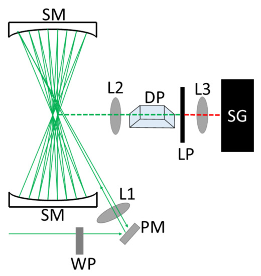
Figure 1.
Experimental setup for measuring the spectrum of N and O consists of: WP: half waveplate PM: planar mirror, L1: focusing lens (f = 150 mm), SM: spherical concave mirrors (f = 50 mm), L2: plano-convex lens (75 mm), L3: plano-convex lens (250 mm), DP: dove prism, LP: long-pass filter, SG: spectrograph.
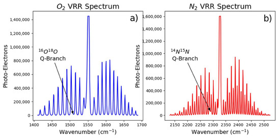
Figure 2.
Spectra taken in the vicinity of the fundamental band of molecular (a) oxygen and (b) nitrogen with 60 s integration time.
Data analysis was performed using custom Python scripts. First, baseline subtraction was performed in post-process using linear regression, and then we corrected for the line intensity dependence of the VRR spectra (see Equation (1) below). Optical corrections were then applied to account for the wavelength dependent properties of the spectrograph’s optical components as provided by the manufacturer. This included the quantum efficiency of the CCD sensor, the reflectivity of three mirrors, and the efficiency of the diffraction grating. Cosmic rays removal was performed by comparing each exposure to the average of all exposures, and any pixel with signal outside of a three sigma limit within each exposure was replaced with the median value over all exposures. Integration of each peak was performed using the trapezoid method, with the center point of each integration range being determined by reconstructing the spectrum using cubic interpolation. While the lines within a single branch were integrated using the same integration width, the integration width varied between different branches of the VRR spectra. These integration ranges were determined by minimizing uncertainties related to line overlap. Broadening affects due to changes in temperature should not change these integration ranges. The perceived broadening of the Raman lines is entirely due to instrumental resolution, and broadening changes as a function of . Broadening will remain significantly less than our instrumental resolution for any atmospherically relevant temperature.
2.2. High-Resolution Raman Spectra of Molecular Oxygen and Nitrogen
From Figure 2 we can see that care must be taken when selecting lines to determine temperature. VRR lines in the immediate vicinity of the Q-Branch need to be avoided due to the overlap biases. The lines to be avoided include and of the S-branch and O-branch of N, respectively. The same can be said for and in O S-branch and O-branch, respectively. We also avoid using lines that overlap with the pure vibrational Raman lines of isotoplogues NN and OO. The isotopologues vibrational lines overlap with and in the O-branch of N and O, respectively. Near room temperature, the maximum Raman intensity is measured at and for N and O respectively, after which the intensity decreases quickly. Furthermore, N lines with even J are more favorable due to their higher intensity with respect to odd numbered lines due to nuclear spin degeneracy. Therefore, for N, we will focus on even lines within the ranges of 2132–2306 cm (O-branch, ) and 2355–2523 cm (S-branch, ). The analysis for O will focus on the lines within the ranges of 1413–1533 cm (O-branch, ) and 1575–1689 cm (S-branch, ).
2.3. Comparison of Methods for Inferring Temperature
Atmospheric temperature was determined from 24 separate spectra, 11 from O and 13 from N. For each experiment, the thermocouple was used to determine the temperature of the room. However, as mentioned earlier, the thermocouple was positioned about a meter from the scattering volume. This was because we wanted to avoid light scattered off of the thermocouple from entering the spectrograph. To ensure room temperature was measured, we ensured the thermocouple was not in contact with the optical bench. Even if the thermocouple were closer to the scattering plane, it would have been difficult to determine, with high accuracy, the temperature in the scattering region. In fact, 400 W of continuous-wave laser power was focused onto the scattering region of the multi-pass cell (10 W × 40 passes). Therefore, the thermocouple readings are not ideal for determining the accuracy of the temperature values determined from the VRR spectra. We still use the thermocouple for comparison throughout the paper; however inter-comparisons of Raman derived temperatures are our primary tool in determining the precision and self-consistency of our approaches. By comparing rigid rotor and non-rigid rotor derived temperatures to the thermocouple we show how agreement between the Raman and thermocouple temperatures can be improved using non-rigidity corrections. However, by comparing temperature derived from the S-branch to temperature derived from the O-branches we show that non-rigid rotor corrections are also necessary for Raman-based inferred temperatures to be self-consistent, or be in agreement with each other.
Of the four methods, we first use the fitting of integrated intensities of the individual VRR lines within the O- and S-branch from each spectra to determine temperature. The temperatures derived from fitting line intensities within the S- and O- branch are compared to each other to determine self-consistency and precision of the fitting method. To test self-consistency we take the mean of the temperature difference for two different methods over all spectra analyzed. Precision is determined by taking the standard deviation of the temperature difference for two different methods over all spectra analyzed. Throughout Section 3 each method derived to infer temperature from VRR spectra is compared to the temperature determined by the fitting method. We choose to use the fitting method as the reference because it incorporates all viable lines within a branch and has been previously used to determine temperature in both PRR and VRR temperature applications [12,23,29]. These comparisons are branch specific, meaning that a measurement method that uses VRR transitions from the S-branch of Nitrogen is compared to the temperature and uncertainty determined from the fitting of the S-branch of Nitrogen, etc. In Section 4 we explore the self-consistency and precision of all methods performed and look at how each method correlates as the temperature in the room changes.
3. Results
3.1. Temperature Dependence of a Rigid Diatomic Molecule.
The Raman signal from a single vibro-rotational transition v = 1 ← v = 0, J + 2 ← J, measured in units of number of photons, taken at temperature T is equal to [20]:
where A includes all fundamental constants and factors accounting for the scattering geometry common to all vibro-rotational Raman lines, is the cross section common to all rotational transitions within the rigid rotor approximation, N is the total number of molecules, is the nuclear spin factor associated with a rotational quantum number J, is the energy of the rotational state J, and is the frequency of the Raman line corresponding to the vibrational quantum numbers v and the rotational quantum number J. is the rotational and vibro-rotational line strength which differs for the S-branch and the O-branch:
Finally, the partition function, , represents the sum over all rotational states:
In the case of O, the nuclear statistical factor, , is equal to 0 for even J, and equal to 1 for odd J, while for N, is equal to 6 for even J, and 3 for odd J. The alternating intensity of N and the absence of even rotational states of O seen in Figure 2 is a direct result of . is measured in units of number of photo-electrons and carries a counting error of . The term corrected for the wavelength dependent optical efficiency of the spectrograph and the dependence in Equation (1) is denoted with a prime .
3.2. Least-Squares Regression of VRR Line Intensity
We follow the method of temperature estimation from fundamental Raman bands of N and O first derived by James and Klemperer [30] and later used by Asawaroengchai and Rosenblatt [25]. The rigid-rotor form of the equation can be derived from Equation (1):
The left hand side of Equation (4) is the dependent variable, while the energy, , is the independent variable. The logarithm on the right side of the equation includes only constants, and therefore, forms the intercept. Temperature can be extracted from Equation (4) using linear least-squares regression. We show an example of these fits in Figure 3 where we infer temperature by fitting integrated VRR transitions of N. For these fits, we did not include lines directly adjacent to the pure vibrational line and those overlapping with the primary isotopologue’s vibrational line. For N, only the lines with even rotational quantum numbers were used in the fits to reduce the effects of bias from overlapping lines.
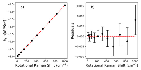
Figure 3.
Temperature can be determined by fitting the intensity of individual lines. (a) The temperature is inferred from the S-Branch of N from the inverse of the slope. The error bars are much smaller than the data markers. (b) The residual plot shows that the uncertainty is comparable to the residuals.
Least-squares regression was performed on integrated line intensities from each of the O and N VRR spectra. Each fit was optimized by minimizing the statistic. Over all of the experiments and , suggesting good agreement between model and data. In Table 1 we show the statistics of comparing the results from each branch to the thermocouple (TC), as well as temperatures derived from each branch to each other. On average the temperature determined using the S-branch and O-branch of both gases differ significantly. These differences vary only a small amount, as shown by the standard deviation of the differences between S- and O- branch temperatures in Table 1. Additionally, none of the fitting derived temperatures are in agreement with the room temperature measured by the thermocouple. The low temperature values inferred from the S-branch of both gases suggest that the intensity of lines are decaying faster with respect to J than predicted by the rigid-rotor approximation in the S-Branch. Meanwhile, the high temperature values inferred from the O-branch of both gases suggests the intensity of lines are decaying slower with respect to J than predicted by the rigid-rotor approximation in the O-Branch.

Table 1.
Comparisons of temperatures derived from fitting VRR line intensities and measured using thermocouple (TC) when molecules are assumed to be rigid-rotors. The columns from left to right are the mean difference of the S-branch and thermocouple temperatures, the O-branch and thermocouple temperatures, the mean difference of the S- and O-branch temperatures, and the standard deviation of of the difference of S- and O-branch temperatures.
3.3. Temperature Dependence of the Non-Rigid Diatomic Molecule
The results in the previous section suggest that the Raman cross-section is dependent on the rotational quantum number. In this sub-section we will demonstrate how treating O and N molecules as non-rigid rotors can improve the agreement between the two branches of the VRR spectra for both gases. The rigid-rotor approximation assumes that there is no vibrational-rotational coupling during a vibro-rotational transition. It has been shown, however, that this is not the case for the vibro-rotational spectrum of N and O [25,28,30,31]. These works showed that the ratios of S- and O- Branch line intensities with the same initial rotational state diverged from the rigid rotor approximation. This divergence is dependent on the quantity , defined as [25]:
where and are the polarizability anisotropy and its first derivative at the equilibrium inter-nuclear distance . Recently, we reported new, more accurate, measurements of obtained from Raman spectra of fundamental bands of molecular O and N [28]. We report these values in Table 2. The dependence of line intensities on vibro-rotational interactions can be effectively accounted for using the first-order approximation of the Herman-Wallis factor, [25,32]:
where for the S-branch and for the O-branch. The quantity is twice the ratio of the rotational constant of the molecule () and its zero-point vibrational energy () [31]. The values for and can be found in Table 2. The subscript designates the fundamental band.
Table 2.
Molecular constants used in non-rigidity corrections for O and N. These are the rotational constant (), zero point vibrational energy (), the polarizability anisotropy ratio (), and the uncertainty in the anisotropy ratio ().
3.4. Applying Non-Rigidity to Least-Squares Regression
The Herman-Wallis correction factor acts as a J-dependent modification of the intensity of a vibro-rotational transition. We can modify Equation (4) to reflect this correction:
where we designated the intercept from Equation (4) as , and the non-rigidity correction has been incorporated into the left-hand side of the equation with the other J-dependent parameters. As can be seen from Table 3, the inclusion of the non-rigid rotor correction greatly improved the agreement between the temperatures inferred from the S- and O- branches of both gases. The quality of the fits are still high, with each fit having an and a in each of the fits. However, the mean difference in temperatures from the N branches is 3.0 K, with temperature inferred from the O-branch being the highest. While it is still unclear what the source of this discrepancy might be, it may be related to the difficulty in resolving the N VRR spectra (which we discuss with more detail in Section 4.1). However, the precision of the measurement can be as good as 0.3 K. The O measurements are in much better agreement; however, the uncertainty of the O-branch measurement is much larger than its S-branch counterpart. This could be the result of the O-branch having less viable VRR lines than the S-branch resulting in fewer degrees of freedom while fitting. Considering the agreement between the two branches is 0.3 K we can say that the fits of O’s VRR line intensities are consistent to within 0.3 K and a precision of 0.3 K. The agreement of the temperatures inferred from VRR spectra and those measured using the thermocouple also significantly improved as a result of incorporating the non-rigidity correction.
Table 3.
Statistical comparisons of temperatures and uncertainties determined from fitting VRR line intensities. The columns, from left to right, are the gas, the mean difference of the S- and O-branch temperatures (), the standard deviation of the difference between the S- and O-branch (), the mean uncertainty of the S-branch temperature (), and the mean uncertainty of the O-branch temperature ().
3.5. Deriving Temperature from Two Isolated Lines
By taking a ratio of the integrated intensities of two distinct VRR transitions, the temperature term in Equation (1) can be isolated. For optically corrected intensities of VRR lines with rotational quantum numbers and the ratio, is:
where is a ratio of the vibro-rotational line strengths:
rearranging Equation (8) yields:
The ratio includes the previously discussed corrections in addition to the non-rigidity corrections:
This formulation can be applied to any two-line combination in the VRR spectrum.
Propagation of Uncertainty in Temperature
We identified several sources of uncertainty that are accounted for in our analysis. Numerical integration is employed to quantify the intensity of each line. Due to the limited resolution of the spectrograph, the VRR lines overlap on the edges. This means that each integral is biased by signal from the Raman lines adjacent to it. We refer to this uncertainty as adjacent line bias. We estimated these uncertainties by fitting each spectra with a series of Gaussian functions, one for each VRR line. Adjacent line bias was estimated by integrating the contribution from all adjacent Gaussian functions within the range of integration for a particular line. Another source of uncertainty is the numerical integration, performed using the trapezoidal rule. Integration ranges were chosen for each branch and gas such that the sum of these three uncertainties were minimized. For N, the integration ranges were chosen to be 8.6 cm and 7.6 cm wide for the O- and S-branch lines, respectively. The integration ranges for O were chosen to be 12.2 cm and 10.4 cm for the O- and S-branch lines, respectively. We also include the random uncertainty associated with the photon counting statistics (square root of the number of photons):
The only variables carrying an appreciable amount of uncertainty in Equation (10) are the experimental ratio of Raman line intensities, and the non-rigidity correction, . The energies of corresponding transitions have been measured before and are known with accuracy better than 6 digits [34,35]. We can therefore propagate the uncertainties using the following relation:
Computing this derivative in Equation (13) we have:
The uncertainty is directly proportional to the relative uncertainty of the corrected line ratios. The relative uncertainty of the corrected line ratios, , simplifies to the summation in quadrature of the relative uncertainty of the line intensities as well as the relative uncertainty in non-rigidity corrections. From this, it can be seen that selecting lines with high intensity is favorable, as these lines will tend to have the lowest uncertainty relative to the intensity. However, intensity is not the only consideration when selecting lines. Using Equation (10), the uncertainty can be simplified to:
where the uncertainty in is determined from the uncertainty of the two lines using Equation (12). We can now see that the uncertainty is dependent on temperature and the difference in transition energy of each state. The uncertainty of temperature increases quadratically with temperature, leading to reduced accuracy as temperature increases. This can be counteracted by selecting lines that are far apart, effectively increasing the difference in energy between the two states. When temperature increases, lines with low rotational quantum number decrease in intensity while lines with high rotational quantum number increase in intensity. When two lines are spectrally close, meaning the difference in their transition energies is low, the relative change in intensity of one line in comparison to the other is small. The resulting ratio of intensities is less sensitive to changes in temperature for two lines with small differences in transitional energy than two lines with large differences.
3.6. Two-Line Ratio Method
The temperature was inferred from every possible line combination within the chosen spectral window. This includes using two lines from the S-Branch, two lines from the O-Branch, as well as one line from each branch. In Figure 4 and Figure 5, we compare the temperature values calculated using Equation (10) for every line combination to the values inferred from the least-squares fit for each experiment. Figure 4 focuses on temperatures derived from two-line, different branch, ratios (TLDR), while Figure 5 focuses on temperature derived from two-line, same branch, ratios (TLSR). In each figure, we plot the mean difference between every temperature values calculated from the two line ratio and those temperature values inferred by fitting VRR line intensities. Several lines in Figure 4 and Figure 5 are consistent and have a precision with respect to the fitting method of less than 1 K. We define the consistency with respect to the fitting method as the mean of the temperature differences for each line combination over all experiments, whereas the precision with respect to the fitting method is defined as the standard deviation of the temperature differences over all experiments. Table 4 compares the total number of lines that meet this 1 K requirement to the total number of lines for each gas and branch. Overall, the S-branches for both gases have a greater number of line combinations that meet the 1 K criteria than their O-branches or TLDR counterparts. The Nitrogen S-branch includes the highest number of line combinations that meet the 1 K criteria, while Oxygen S-branch includes the highest percentage of lines meeting the 1 K criteria. The O-branch for each gas has a lower percentage of lines meeting our criteria because of greater overlap with the pure vibrational line, as well as, the overlap with the Q-Branch corresponding to the second most abundant isotopologue. The TLDR method is comparable to the TLSR methods applied to the O-Branch in terms of the percentage of lines meeting our 1 K criteria for both gases.
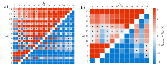
Figure 4.
Mean temperature difference between the temperature derived from the two line, different branch, method and the average of the the least-squares method results for: (a) Nitrogen and (b) Oxygen. Black dots represent line combinations where the mean temperature difference and standard deviation of the temperature difference were both less than 1 K.
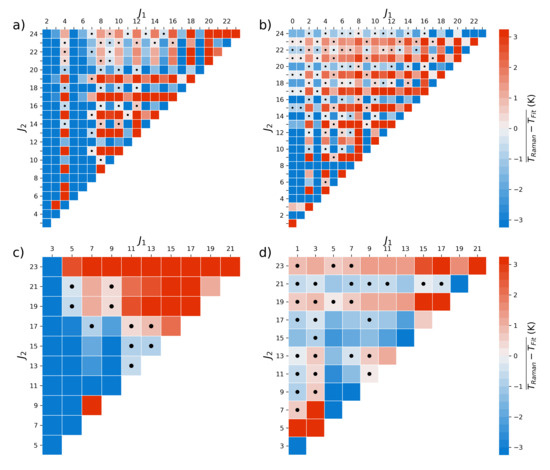
Figure 5.
Mean temperature difference between the tempreature derived from the two line, same branch, method and the least-squares method for the: (a) Nitrogen O-branch, (b) Nitrogen S-branch, (c) Oxygen O-branch, (d) Oxygen S-branch. Black dots represent line combinations where the mean difference and standard deviation of the difference are both less than 1 K, same as Figure 4.
Table 4.
Summary of the two-line ratio method applied to two S-Branch lines (S), two O-Branch lines (O), and one line from each branch (TLDR). Here we show the total number of line combinations (), the number of line combinations that meet the <1 K criteria (), and the percentage of lines that meet this criteria. This table summarizes Figure 4 and Figure 5 above.
In Table 5 we show the lines with the lowest absolute mean difference compared to temperature values determined by fitting VRR line intensities. Each of these line combinations is within 0.3 K of the fit inferred temperatures. The precision of each line with respect to the fit inferred temperature values is less than 0.7 K in each case. The line combinations with the best precision with respect to the fit derived temperature values are listed in Table 6 for each branch. The standard deviation is 0.3 K or less for each of the branches, and the mean differences for each of the lines are 1.0 K or less for everything but the N TLDR result. It is also worth pointing out that the lines with the greatest precision are separated by at least 10 rotational quantum numbers.
Table 5.
Line combinations with the lowest mean difference between the two-line ratios and the temperature values inferred from fitting. The columns are the gas and branch (in parentheses) temperature was inferred from. Two-line, different branch, columns are designated by TLDR. The rows, in order, are the line combination (), the mean temperature difference (), the standard deviation of the temperature difference (), and the mean uncertainty of the two-line same branch method (). For the TLDR columns the S-branch line is designated by and the O-branch line is designated by .
Table 6.
Line combinations with the lowest standard deviation for the difference between the two line ratio temperature values and the “fit inferred” temperature values for each gas and branch. The rows and column labels follow the same convention as Table 5.
As previously discussed, uncertainty is inversely proportional to the difference in rotational transition energies, or the wavenumber separation of the two VRR lines used. This is illustrated in Figure 6, where a clear decrease in mean temperature difference and variability is observed as the separation between the two lines increases. This shows that a line combination is more likely to have high consistency with respect to the fitting method as the two lines become more separated, but does not preclude a line combination with lower separation. As can be seen, there are several line combinations in the range cm that are consistent with the fit to within 1 K with respect to the fitting method. Figure 7 shows a more detailed summary of the uncertainty calculations. Line combinations with the greatest separation appear in the upper left-hand corner of each plot. While there are some exceptions, such as line combinations involving lines that overlap with the pure vibrational lines, the estimated uncertainty is lower for line combinations closer to the upper left-hand corner of each plot. For N, many of the line combinations involving odd rotational quantum numbers have higher uncertainty. This is likely due to these line combinations having higher relative uncertainty from lower photon statistics and greater sensitivity to overlap from neighboring lines.
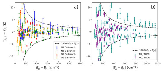
Figure 6.
The mean difference between temperature values determined using the (a) two line, same branch, and (b) two line, different branch, methods and temperatures inferred from fitting for all spectra analyzed. Error bars represent the standard deviation of the temperature difference across all spectra. The dashed lines are used as a guide to illustrate the inverse relationship between the variability in temperature difference and energy difference. It should be noted that using Equation (15), this line is equivalent to a relative uncertainty in the line ratio of 0.003.
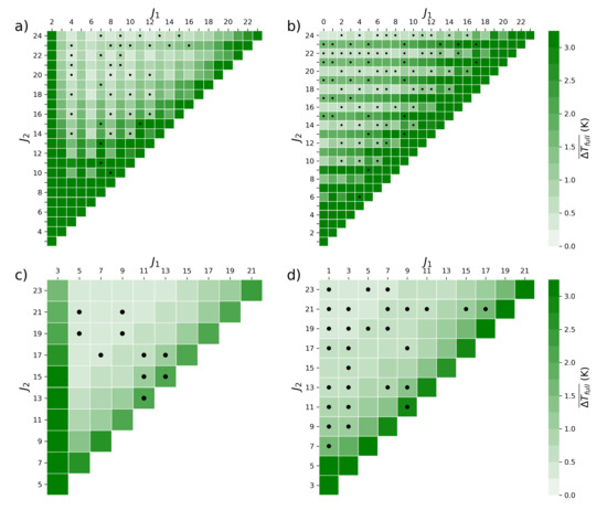
Figure 7.
Average of uncertainty estimated using Equation (15) for: (a) Nitrogen O-branch, (b) Nitrogen S-branch, (c) Oxygen O-branch, (d) Oxygen S-branch. A black dot in a box represents line combinations where the mean difference and standard deviation of the difference are both less than 1 K, same as Figure 4.
3.7. The Multi-Line Ratio Approach
So far, we either relied on taking the ratio of two isolated lines, or fitting the intensity of a collection of isolated lines. However, this can be impractical as isolating single lines requires a polychromator and a photo-detector array with high enough resolution to fully resolve each line. In applications that infer temperature from PRR spectra, it is more typical to use photomultipliers to measure the light transmitted through narrow-band interference filters. These filters isolate two sections of the PRR spectra, each section including multiple lines. In addition to its simplicity, a major advantage of this type of setup is that each photodetector is measuring a higher signal resulting in greater precision in comparison to the methods employing ratios of two isolated PRR lines. Finally, the typical transmission of filters is significantly higher than that of a polychromator system. Inspired by this approach, and building off of the theoretical work above, we derived a means of inferring temperature by taking a ratio of two regions within the VRR spectra.
We follow a similar approach to how we derived temperature from two isolated lines in the same branch. The energy of a line with rotational quantum number , where i is an integer, is related to the energy of a line with rotational quantum number, J, through the following relation:
where and are rotational and centrifugal distortion constants respectively. The values for these constants were determined for O by Fletcher and Rayside [34], while Bendtsen [35] determined them for N. Using Equation (1), corrected for the contribution, we can represent the intensity of adjacent lines using a summation:
If we take the ratio of two sections of the VRR spectra, the first beginning at and including lines and the second beginning at and including lines we get
We can then obtain an expression for temperature that is similar to Equation (10):
Determining temperature with this formulation requires an iterative approach, similar to the multi-line analysis of Salzman, Masica, and Coney, due to the dependence of on temperature [36]. The analysis to determine temperature can be performed by calculating using a starting temperature value, , that is above 0 K. This can be repeated to calculate from , and then repeated continually until was less than the desired tolerance (we use 0.001 K), where is the total number of iterations. The calculation converges to the final temperature value for any reasonable starting temperature; however, the number of iterations needed to calculate the final temperature is dependent on the difference between the final temperature and the starting temperature. We report results using K, but found that we get the same results when is 1 K, 290 K, and 350 K. Using Figure 5, we were able to identify two sections of each VRR branch by selecting regions where line combinations are most consistent and precise with respect to the fit inferred temperatures (black dots). This was somewhat difficult for the O-branch of O, as the lines most in agreement with the fitting method were overlapped by the Q-line. We were forced to use two small sections of the signal that were not spaced far apart. While the calculation can be performed on sections of different sizes, we opted to report calculations with two evenly sized sections of the spectra. We performed the analysis on each branch, and we report the lines used, and wavenumber ranges in Table 7.
Table 7.
Parameters used to determine the temperature from each branch in the VRR spectra for O and N using the multi-line ratio method. The top row shows the gas and branch (in parentheses). The rows represent the rotational quantum number (J) and wavenumber ranges () used to estimate temperature using the multi-line ratio formulation.
Table 8 shows that the multi-line ratio temperature values were consistent with respect to the fitting method to within 1 K, even for the O-branch of O. However, limitations on the O-branch of O lead to lower precision than the other branches. A maximum of 5 iterations were needed in order to satisfy the minimization condition of the calculation. We have not seen any relation between the number of lines included in the calculation and the number of iterations required for convergence. The convergence appears stable, even when the number of iterations are increased well beyond the precision requirement. We also successfully applied the method to include different line counts in each part of the ratio. Comparing Table 8 to Table 5 and Table 6 we can see that the precision with respect to the fit inferred temperature values is comparable to that of the best line combinations using the TLSR method. We assume adjacent line bias uncertainty to be negligible compared to photon statistics, so the intensity ratio’s relative uncertainty, , reduces to the sum of inverse intensities. The uncertainty in temperature is calculated iteratively, starting with a null uncertainty. The only non-negligible sources of uncertainty in are related to the non-rigid rotor corrections and each iteration’s temperature. The mean uncertainty calculated across all experiments were comparable for all four branches.
Table 8.
Comparison of the multi-line ratio approach to inferring temperature with the fitting method. The columns represent the gases and branch (in parentheses) used for inferring temperature. The rows in order on the number of iterations (), the mean difference of the multi-line ratio and fitting methods (), the standard deviation of the multi-line ratio and fitting methods (), and the mean uncertainty of the multi-line ratio method ().
4. Discussion
4.1. Comparing Methods of Inferring Temperature
We derived and implemented four methods to infer temperature from the VRR spectra of N and O and discussed their performance when compared to the least-squares regression method. We now broaden the scope of our analysis by comparing each of the methods described above with each other, as seen in Figure 8. We found that the temperatures determined by fitting the S- and O-branch of N disagreed by at least 2.5 K. The reason for that is probably related to the fact that the VRR spectra of is less resolved than those of O thus making the determination of the single line intensity less reliable. In particular, the resolution limitations might have affected the determination of from the VRR analysis, which was calculated from the same setup. We found that if a value of for N is used, the difference in temperature values determined from fitting O- and S- branches separately drops to only a few tenths of a Kelvin. There is generally strong agreement between different measurement methods when comparing the results of the same VRR branch (<0.4 K) which indicates that a greater degree of consistency is attainable from the N VRR spectra with improved instrument resolution.
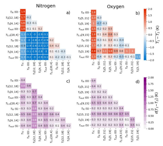
Figure 8.
Comparisons of all the methods used to infer temperature from the VRR spectra are listed as: (a) The mean difference of all methods applied to the N VRR spectra. (b) The mean difference of all methods applied to the O VRR spectra. (c) The standard deviation of the difference of all methods applied to N. (d) The standard deviation of the difference of all methods applied to O. The temperature measurements compared are those from a collocated thermocouple (), fitting ( (branch)), two-line, same branch, ratio (), two-line, different branch, ratio (), and multi-line ratios ( (branch)).
The comparative precision across all methods was ≤0.9 K for all cases involving the N VRR spectra. Comparing the multi-line ratio and the fitting for the S-branch of N suggests precision values as low as 0.1 K with respect to each other (consistent to within 0.2 K). Comparatively speaking, the different VRR methods are in much better agreement for O than for N. Several are within 0.1 K of each other and most fall within 0.5 K. The precision of these methods in comparison to each other is generally within 0.5 K, with the exception of the two-line ratios. It is apparent from Figure 8 that the two-line ratio method is generally worse in terms of precision in comparison to its counterparts for both gases, as we already noted earlier. Table 4 shows that the two-line ratio method is best applied to the S-Branch, as a lower proportion of lines were found to meet the <1 K criteria for the O-Branch and cross-branch estimates. Again, the most precise comparison (0.1 K) is found by comparing the S-branch fit with the the S-branch multi-line ratio approach. Fitting, two-line ratios, and multi-line ratios are precise to within 1 K when applied to the VRR spectra of O. Additionally, each of these methods showed a high level of self-consistency to within 1 K.
Overall, the methods we derived performed better when applied to O VRR spectra than when applied to N VRR spectra. While N has greater abundance in the atmosphere, and therefore greater overall Raman signal, than O, the intensity of the lines within the O spectrum are comparable to N VRR transitions with even rotational quantum number. This is due largely to the nuclear spin statistic, , which results in molecules having both even and odd rotational quantum number for N and only odd rotational quantum number for O. Another effect of is that the lines in the O VRR spectrum have greater separation, are easier to resolve, and less prone to adjacent line bias. Uncertainty due to adjacent line bias can be reduced by using methods that employ multiple lines, such as fitting the intensities or the multi-line ratio. However, high degrees of self-consistency and precision (<0.5 K) were still achievable using two line ratios. Additionally, the precision of temperature values inferred from VRR spectra were small enough that temperature changes could be resolved over a relatively small temperature range.
4.2. Temperature Variation and Correlation
Across all experiments, the ambient temperature varied from 292.2 K to 293.3 K as measured by the thermocouple. Figure 9 compares the different methods we employed plotted with the ranked thermocouple readings. Most of the temperatures determined from Raman methods fall within the 95% confidence range of the thermocouple. As temperature increased in the room, increasing trends were also observed for the Raman calculations with varying degrees of correlation, as shown in Figure 10. Generally speaking, each comparison shows a positive correlation and similar slopes over the temperature range explored. However, the correlations are higher for methods applied to O VRR spectra than N VRR spectra, especially the methods that involve two line calculations. This is likely due to isolating single lines in the N spectra being more difficult than for O. Overlap from adjacent lines reduces the overall precision of temperatures determined from isolated lines in the N spectra. Additionally, temperature values inferred from the O VRR spectra correlate better with the thermocouple than those inferred from the N VRR spectra.
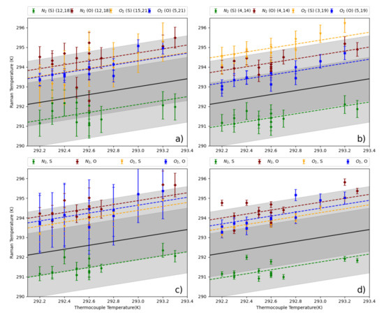
Figure 9.
Temperature inferred from the VRR spectra plotted against the ranked temperature measured by the thermocouple, described by the following: (a) The line combinations most consistent with fitting method using the two-line, same branch, ratio. (b) Most precise line combinations with respect to the fitting method using two-line, same branch, ratio approach. (c) The temperature derived from fitting the VRR line intensities. (d) Temperatures determined by taking a ratio of multiple lines. The dark gray regions in each plot represent the 1 uncertainty of the thermocouple (1.1 K) and the light gray regions represent the 2 uncertainty. The lines represent a line with a slope of 1.0, and linear regression was used to determine the offset with respect to the thermocouple.
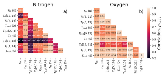
Figure 10.
Pearson’s correlation matrix composed of every method used to predict temperature from the VRR spectra of: (a) N and (b) O. Labelling follows the same convention as Figure 8.
4.3. Additional Sources of Uncertainty
Temperatures determined from the S- and O- branch of O, along with the O-branch of N, are 1–3 K higher than those measured by the thermocouple. Furthermore, the temperature values determined from these three branches are in fairly good agreement with each other. Despite large power densities in the scattering region, localized heating is unlikely. We estimate that over a 15 min exposure the temperature in the scattering region would only increase by 0.003 K at most. This estimate takes into account heating due to linear absorption, which is 0.2 Mm in the atmosphere at 532 nm, and heat dissipation [37,38]. Effects involving the motion of air in the room, the buoyancy of heated air, or absorption effects of aerosol were not considered. The first two effects would mitigate localized heating, and the the third effect would increase localized heating, the effect is likely small. Again, most of the temperature values determined by analyzing the VRR spectra of O and N are within 2 of the thermocouple’s accuracy.
The instrumental transfer function, or the wavelength dependent intensity sensitivity of the detector in the spectrograph, represents a source of uncertainty in these experiments. The transfer function can be estimated experimentally by exposing the spectrograph to a black-body source or spontaneous emission from luminescent glasses [39]. These systems are often expensive, difficult to implement properly, and correction calibrations need to be performed often. These techniques can help diagnose the effects of distortions due to hot spots and etaloning (which is more of an issue in the near-infrared) [40]. Unable to perform these calibrations, we estimated the instrumental transfer function using the specifications of the spectrograph provided by the manufacturer. It is possible that the VRR transitions themselves could be used to improve this calibration in the future. Raj et al. recently showed how an intensity calibration could be performed using the intensity of PRR and VRR transitions [41]. Additionally, further improvements could be achieved with a better alternative temperature measurement and by exploring a wider temperature range.
4.4. Generalizing the Results
We employed several methods of estimating atmospheric temperature from the VRR spectra of N and O. These methods can be applied toward the development of instrumentation that can remotely infer temperature in turbid environments. In such applications, the investigated temperature values might be different, and the ranges might be wider than the temperature values we explored in this work. However, because our methods are reliant on the temperature dependence of the rotational states of a canonical gas through the Boltzmann distribution, these methods can be generalized to a greater range of temperatures. For two-line ratios a specific line pairing may only be appropriate for specific temperature values, especially if the intensity of one line becomes too small for a sensitive measurement to be made. The optimal line pairings for atmospherically relevant temperatures should be similar to those discussed in this work as the intensities will not deviate enough to make them less sensitive. These optimal line pairings can be estimated using an approximated form of Equation (1):
where is the rotational constant from Section 3.7. The most intense line in the VRR spectra is for , or . As a consequence, if and are the optimal J values obtained by comparing two single lines at , then, the optimal J values at a different temperature T should be and . In the same vein, the optimal line pairs of one gas can be estimated from the results of another, because J should scale as . From Table 5, we can surmise that [12, 18] is the optimal line pairing for N when compared to the fitting method; plugging this line pairing into the relation, we estimated that for O, the optimal values = [14.1, 21]. Since the O VRR spectra only includes odd-J valued lines it can be surmised that the estimated optimal line pairing for O is [15, 21]. This indeed, is the line pair that we found to be most in agreement with the fit for the S-Branch of O, as per Table 5, supporting our argument. Therefore, we used this method to calculate estimated optimal line pairs for determining the temperature for different temperature regimes and report the values in Table 9.
Table 9.
Estimates of the optimal line pairing for the two-line ratio method using the results from Table 5. These calculations were referenced to a temperature , as discussed in the text, of 293 K.
Similar conclusions can be extended to the multi-line ratio and line fitting methods as well. The multi-line ratio incorporates a greater number of photons compared to the two-line ratio methods, and therefore should be more sensitive across a greater range of temperatures. However, the ideal line groupings may change in a similar fashion to the two-line ratio method discussed above. The temperature range of the line fitting method is largely limited to the spectral range of the spectrograph used. Line selection is less important for this method as well, since the method is performed by minimizing the -statistic. This method is dependent on the relative uncertainty of each line, and so would favor the lines with the highest intensity in the spectral range of the instrument.
The value of in the non-rigidity correction should be applicable to temperature regimes not explored in this work. There is no theoretical basis for temperature dependence of , though experimental work should be performed to confirm this theoretical prediction [30,31,32]. Typically, experiments to determine are performed at room temperature, and these measurements are in-turn used to determine temperature at different temperature regimes [25,28,42,43]. It has been shown that these room temperature determined values do improve the accuracy of temperature measurements at flame temperatures [12,22].
5. Conclusions
Our experimental setup and measurement procedure allowed for high resolution measurement of VRR spectra of N and O. Using the fundamental properties of these molecules, we were able to determine atmospheric temperature within the scattering region of our multi-pass cell. For both gases, treating the molecules as non-rigid rotors not only improved the self-consistency of temperature derived from Raman measurements, but also improved the the agreement between Raman derived temperatures and the thermocouple. However, the VRR spectra of O, specifically the S-Branch, would be best for determining atmospheric temperature with high precision without the need for ad hoc temperature calibration. The S-Branch provided the best results in this work, largely due to higher line intensities and a greater number of viable lines due to less influence from overlapping vibrational lines. We found that greater resolution is likely needed when determining temperature from individual N lines. A more accurate estimate of might further improve the temperature inferred from N VRR spectra. Regardless, the N S-branch would likely provide the most precise temperature measurement for applications where a calibration can be performed. This is because this branch would have the strongest signal out of the four branches explored.
We derived four methods of ascertaining atmospheric temperature from the VRR spectra of N and O. These methods could be a starting point in the development of an instrument for contactless measurements of atmospheric temperature using VRR spectra of N or O, though further work is necessary to scale these methods to a field deployable instrument. Our analysis to find the optimal line combinations was performed for a limited range of temperature values. The best line combinations will need to be revisited for different temperature regimes and we provided a theoretical approach to estimate the optimal line pairs. However, our work shows that regardless of temperature, well separated line combinations are ideal. Of the methods implemented in this work the multi-line ratio is the best in terms of attainable precision and practical applicability. A future implementation would still require well-characterized filters that isolate specific line combinations. A calibrated version of the multi-line method can also be envisioned, where two sections of the spectra are isolated and a calibration constant allows for temperature to be determined, just like in PRR methods. We anticipate that the VRR method would be applicable to the same range of temperatures that purely rotational Raman can be, since the formulation is similar. Methods employing interference filters would have orders of magnitude greater transmission than our spectrograph setup, which would allow for higher time resolution. It would be interesting to apply such a setup to investigate the effects of temperature fluctuations on atmospheric processes. Line-fitting and two-line ratios can also be effective techniques, though they may only be viable options when using a polychromator or other light dispersion techniques. These methods do not have the strict filter requirements of the multi-line method.
It is worth reiterating, again, that VRR-based temperature measurement will not replace PRR-based temperature measurements. However, we believe there are situations where the elastic scattering signal will be too strong for PRR-based measurement to be reliable. Determining temperature from VRR spectra may be useful in the development of short range LiDAR systems that investigate turbid environments, such as near clouds. Additionally, VRR spectra could be used for temperature measurements in combustion diagnostics, especially in cases where incomplete combustion leads to the production of particles that could increase the elastic scattering coefficient in the measurement media and degrade the precision of other techniques.
Author Contributions
Conceptualization, M.M., J.B., T.C.; methodology, J.B., C.M.; software, T.C.; validation, M.M., J.B., C.C.; formal analysis, T.C.; investigation, J.B., C.M., T.C.; resources, C.M., J.B.; data curation, T.C.; writing—original draft preparation, T.C.; writing—review and editing, C.M., M.M., J.B.; visualization, T.C., J.B.; supervision, C.M., M.M., J.B.; project administration, C.M.; funding acquisition, C.M., J.B. All authors have read and agreed to the published version of the manuscript.
Funding
This work was supported by the National Science Foundation Division of Atmospheric and Geospace Sciences [grant number ATM1625598]. Partial funding was also provided by The Elizabeth and Richard Henes Center for Quantum Phenomena.
Acknowledgments
Tyler Capek thanks The Elizabeth and Richard Henes for Quantum Phenomena for the Graduate Student Fellowship he received for this work. We acknowledge support from the Michigan Technological University Earth, Planetary, and Space Sciences Institute and Physics Department.
Conflicts of Interest
The authors declare no conflict of interest.
Abbreviations
The following abbreviations are used in this manuscript:
| VRR | Vibrational-rotational Raman |
| PRR | Pure-rotational Raman |
| TLSR | Two line same branch ratio |
| TLDR | Two line different branch ratio |
References
- Easter, R.C.; Peters, L.K. Binary Homogeneous Nucleation: Temperature and Relative Humidity Fluctuations, Nonlinearity, and Aspects of New Particle Production in the Atmosphere. J. Appl. Meteorol. 1994, 33, 775–784. [Google Scholar] [CrossRef][Green Version]
- Platis, A.; Altstädter, B.; Wehner, B.; Wildmann, N.; Lampert, A.; Hermann, M.; Birmili, W.; Bange, J. An Observational Case Study on the Influence of Atmospheric Boundary-Layer Dynamics on New Particle Formation. Bound. Layer Meteorol. 2016, 158, 67–92. [Google Scholar] [CrossRef]
- Kulmala, M.; Rannik, U.; Zapadinsky, E.L.; Clement, C.F. The effect of saturation fluctuations on droplet growth. J. Aerosol Sci. 1997, 28, 1395–1409. [Google Scholar] [CrossRef]
- Nilsson, E.D.; Kulmala, M. The potential for atmospheric mixing processes to enhance the binary nucleation rate. J. Geophys. Res. Atmos. 1998, 103, 1381–1389. [Google Scholar] [CrossRef]
- Chandrakar, K.K.; Cantrell, W.; Chang, K.; Ciochetto, D.; Niedermeier, D.; Ovchinnikov, M.; Shaw, R.A.; Yang, F. Aerosol indirect effect from turbulence-induced broadening of cloud-droplet size distributions. Proc. Natl. Acad. Sci. USA 2016, 113, 14243–14248. [Google Scholar] [CrossRef]
- Chandrakar, K.K.; Cantrell, W.; Shaw, R.A. Influence of Turbulent Fluctuations on Cloud Droplet Size Dispersion and Aerosol Indirect Effects. J. Atmos. Sci. 2018, 75, 3191–3209. [Google Scholar] [CrossRef] [PubMed]
- Bange, J.; Esposito, M.; Lenschow, D.H.; Brown, P.R.A.; Dreiling, V.; Giez, A.; Mahrt, L.; Malinowski, S.P.; Rodi, A.R.; Shaw, R.A.; et al. Measurement of Aircraft State and Thermodynamic and Dynamic Variables. Airborne Meas. Environ. Res. Methods Instrum. 2013, 7–75. [Google Scholar] [CrossRef]
- Muppa, S.K.; Behrendt, A.; Späth, F.; Wulfmeyer, V.; Metzendorf, S.; Riede, A. Turbulent Humidity Fluctuations in the Convective Boundary Layer: Case Studies Using Water Vapour Differential Absorption Lidar Measurements. Bound. Layer Meteorol. 2016, 158, 43–66. [Google Scholar] [CrossRef]
- Laurendeau, N.M. Temperature-Measurements by Light-Scattering Methods. Prog. Energy Combust. Sci. 1988, 14, 147–170. [Google Scholar] [CrossRef]
- Hoffman, D.; Munch, K.U.; Leipertz, A. Two-dimensional temperature determination in sooting flames by filtered Rayleigh scattering. Opt. Lett. 1996, 21, 525–527. [Google Scholar] [CrossRef]
- Haumann, J.; Leipertz, A. Flame-temperature measurements using the Rayleigh scattering photon-correlation technique. Opt. Lett. 1984, 9, 487–489. [Google Scholar] [CrossRef]
- Drake, M.C.; Rosenblatt, G.M. Rotational Raman scattering from premixed and diffusion flames. Combust. Flame 1978, 33, 179–196. [Google Scholar] [CrossRef]
- Cooney, J. Measurement of Atmospheric Temperature Profiles by Raman Backscatter. J. Appl. Meteorol. 1972, 11, 108–112. [Google Scholar] [CrossRef]
- Behrendt, A.; Reichardt, J. Atmospheric temperature profiling in the presence of clouds with a pure rotational Raman lidar by use of an interference-filter-based polychromator. Appl. Opt. 2000, 39, 1372–1378. [Google Scholar] [CrossRef] [PubMed]
- Radlach, M.; Behrendt, A.; Wulfmeyer, V. Scanning rotational Raman lidar at 355 nm for the measurement of tropospheric temperature fields. Atmos. Chem. Phys. 2008, 8, 159–169. [Google Scholar] [CrossRef]
- Wulfmeyer, V.; Hardesty, R.M.; Turner, D.D.; Behrendt, A.; Cadeddu, M.P.; Di Girolamo, P.; Schlüssel, P.; Van Baelen, J.; Zus, F. A review of the remote sensing of lower tropospheric thermodynamic profiles and its indispensable role for the understanding and the simulation of water and energy cycles. Rev. Geophys. 2015, 53, 819–895. [Google Scholar] [CrossRef]
- Lapp, M.; Penney, C.M.; Goldman, L.M. Vibrational Raman scattering temperature measurements. Opt. Commun. 1973, 9, 195–200. [Google Scholar] [CrossRef]
- Keckhut, P.; Chanin, M.L.; Hauchecorne, A. Stratosphere temperature-measurement using Raman lidar. Appl. Opt. 1990, 29, 5182–5186. [Google Scholar] [CrossRef]
- Su, J.; McCormick, M.P.; Lei, L. New Technique to Retrieve Tropospheric Temperature Using Vibrational and Rotational Raman Backscattering. Earth Space Sci. 2020, 7, e2019EA000817. [Google Scholar] [CrossRef]
- Long, D.A. Raman Spectroscopy, 1st ed.; McGraw Hill: New York, NY, USA, 1977; p. 276. [Google Scholar]
- Behrendt, A.; Nakamura, T.; Onishi, M.; Baumgart, R.; Tsuda, T. Combined Raman lidar for the measurement of atmospheric temperature, water vapor, particle extinction coefficient, and particle backscatter coefficient. Appl. Opt. 2002, 41, 7657–7666. [Google Scholar] [CrossRef]
- Utsav, K.C.; Varghese, P.L. Accurate temperature measurements in flames with high spatial resolution using Stokes Raman scattering from nitrogen in a multiple-pass cell. Appl. Opt. 2013, 52, 5007–5021. [Google Scholar] [CrossRef] [PubMed]
- Liu, F.C.; Yi, F. Lidar-measured atmospheric N-2 vibrational-rotational Raman spectra and consequent temperature retrieval. Opt. Express 2014, 22, 27833–27844. [Google Scholar] [CrossRef]
- Buckingham, A.D.; Szabo, A. Determination of derivatives of the polarizability anisotropy in a diatomic molecule from relative Raman intensities. J. Raman Spectrosc. 1978, 7, 46–48. [Google Scholar] [CrossRef]
- Asawaroengchai, C.; Rosenblatt, G.M. Rotational Raman intensities and the measured change with internuclear distance of the polarizability anisotropy of H2, D2, N2, O2, and CO. J. Chem. Phys. 1980, 72, 2664–2669. [Google Scholar] [CrossRef]
- Kiefer, W.; Bernstein, H.J.; Wieser, H.; Danyluk, M. The vapor-phase Raman spectra and the ring-puckering vibration of some deuterated analogs of trimethylene oxide. J. Mol. Spectrosc. 1972, 43, 393–400. [Google Scholar] [CrossRef]
- Borysow, J.; Fink, M. NIR Raman spectrometer for monitoring protonation reactions in gaseous hydrogen. J. Nucl. Mater. 2005, 341, 224–230. [Google Scholar] [CrossRef]
- Borysow, J.; Capek, T.; Mazzoleni, C.; Moraldi, M. Corrections to the Raman fundamental band of N-2 and O-2 due to molecular non-rigidity: Computations and experiment. Mol. Phys. 2019. [Google Scholar] [CrossRef]
- Drake, M.C.; Rosenblatt, G.M. Flame Temperatures From Raman-Scattering. Chem. Phys. Lett. 1976, 44, 313–316. [Google Scholar] [CrossRef]
- James, T.C.; Klemperer, W. Line Intensities in the Raman Effect of 1Σ Diatomic Molecules. J. Chem. Phys. 1959, 31, 130–134. [Google Scholar] [CrossRef]
- Hamaguchi, H.O.; Suzuki, I.; Buckingham, A.D. Determination of derivatives of the polarizability anisotropy in diatomic molecules I. Theoretical considerations on vibration-rotation raman intensities. Mol. Phys. 1981, 43, 963–973. [Google Scholar] [CrossRef]
- Herman, R.; Wallis, R.F. Influence of Vibration-Rotation Interaction on Line Intensities in Vibration-Rotation Bands of Diatomic Molecules. J. Chem. Phys. 1955, 23, 637–646. [Google Scholar] [CrossRef]
- Herzberg, G.; Huber, K.P. Molecular Spectra and Molecular Structure; Van Nostrand Reinhold Company: New York, NY, USA, 1979; Volume 4, pp. 412–498. [Google Scholar]
- Fletcher, W.H.; Rayside, J.S. High resolution vibrational Raman spectrum of oxygen. J. Raman Spectrosc. 1974, 2, 3–14. [Google Scholar] [CrossRef]
- Bendtsen, J. The rotational and rotation-vibrational Raman spectra of 14N2, 14N15N and 15N2. J. Raman Spectrosc. 1974, 2, 133–145. [Google Scholar] [CrossRef]
- Salzman, J.A.; Masica, W.J.; Coney, T.A.; U.S. State; NASA; Lewis Research Center. Determination of Gas Temperatures from Laser-Raman Scattering; National Aeronautics and Space Administration; Clearinghouse for Federal Scientific and Technical Information: Washington, DC, USA; Springfield, VA, USA, 1971.
- Whinnery, J.R. Laser measurement of optical absorption in liquids. Acc. Chem. Res. 1974, 7, 225–231. [Google Scholar] [CrossRef]
- Arnott, W.P.; Moosmuller, H.; Rogers, C.F.; Jin, T.F.; Bruch, R. Photoacoustic spectrometer for measuring light absorption by aerosol: Instrument description. Atmos. Environ. 1999, 33, 2845–2852. [Google Scholar] [CrossRef]
- Hurst, W.S.; Choquette, S.J.; Etz, E.S. Requirements for Relative Intensity Correction of Raman Spectra Obtained by Column-Summing Charge-Coupled Device Data. Appl. Spectrosc. 2007, 61, 694–700. [Google Scholar] [CrossRef] [PubMed]
- Choquette, S.J.; Etz, E.S.; Hurst, W.S.; Blackburn, D.H.; Leigh, S.D. Relative Intensity Correction of Raman Spectrometers: NIST SRMs 2241 through 2243 for 785 nm, 532 nm, and 488 nm/514.5 nm Excitation. Appl. Spectrosc. 2007, 61, 117–129. [Google Scholar] [CrossRef] [PubMed]
- Raj, A.; Kato, C.; Witek, H.A.; Hamaguchi, H.O. Toward standardization of Raman spectroscopy: Accurate wavenumber and intensity calibration using rotational Raman spectra of H2, HD, D2, and vibration–rotation spectrum of O2. J. Raman Spectrosc. 2020, 51, 2066–2082. [Google Scholar] [CrossRef]
- Hamaguchi, H.O.; Buckingham, A.D.; Jones, W.J. Determination of derivatives of the polarizability anisotropy in diatomic molecules II. The hydrogen and nitrogen molecules. Mol. Phys. 1981, 43, 1311–1319. [Google Scholar] [CrossRef]
- Langhoff, S.R.; Bauschlicher, C.W.; Chong, D.P. Theoretical-Study of the Effects of Vibrational-Rotational Interactions on the Raman-Spectrum of N2. J. Chem. Phys. 1983, 78, 5287–5292. [Google Scholar] [CrossRef]


Publisher’s Note: MDPI stays neutral with regard to jurisdictional claims in published maps and institutional affiliations. |
© 2020 by the authors. Licensee MDPI, Basel, Switzerland. This article is an open access article distributed under the terms and conditions of the Creative Commons Attribution (CC BY) license (http://creativecommons.org/licenses/by/4.0/).