Article

Pyramid Pooling Module-Based Semi-Siamese Network: A Benchmark Model for Assessing Building Damage from xBD Satellite Imagery Datasets

1
Center for Applied Statistics, School of Statistics, Renmin University of China, Beijing 100872, China
2
Shenzhen Institute of Artificial Intelligence and Robotics for Society, Shenzhen 518172, China
3
Graduate School of Information Sciences, Tohoku University, Sendai 980-8579, Japan
4
International Research Institute of Disaster Science, Tohoku University, Sendai 980-8579, Japan
*
Author to whom correspondence should be addressed.
Remote Sens. 2020, 12(24), 4055; https://doi.org/10.3390/rs12244055
Submission received: 17 October 2020 / Revised: 7 December 2020 / Accepted: 7 December 2020 / Published: 11 December 2020

Abstract

:
Most mainstream research on assessing building damage using satellite imagery is based on scattered datasets and lacks unified standards and methods to quantify and compare the performance of different models. To mitigate these problems, the present study develops a novel end-to-end benchmark model, termed the pyramid pooling module semi-Siamese network (PPM-SSNet), based on a large-scale xBD satellite imagery dataset. The high precision of the proposed model is achieved by adding residual blocks with dilated convolution and squeeze-and-excitation blocks into the network. Simultaneously, the highly automated process of satellite imagery input and damage classification result output is reached by employing concurrent learned attention mechanisms through a semi-Siamese network for end-to-end input and output purposes. Our proposed method achieves F1 scores of 0.90, 0.41, 0.65, and 0.70 for the undamaged, minor-damaged, major-damaged, and destroyed building classes, respectively. From the perspective of end-to-end methods, the ablation experiments and comparative analysis confirm the effectiveness and originality of the PPM-SSNet method. Finally, the consistent prediction results of our model for data from the 2011 Tohoku Earthquake verify the high performance of our model in terms of the domain shift problem, which implies that it is effective for evaluating future disasters.

Graphical Abstract

1. Introduction

Natural disasters, which have been occurring frequently in recent years [1], pose a huge threat to the safety of residential buildings as well as life and property. Therefore, it is of great significance to obtain accurate information on damaged buildings to carry out interventions after natural disasters [2,3]. Satellite remote sensing technology is used to obtain disaster information because it can acquire rapid and large-scale surface information [4,5,6,7,8,9]. In particular, the recent development of deep convolutional neural network algorithms has improved disaster assessment accuracy based on satellite imagery [7,10,11,12,13,14]. Nevertheless, the practicability of disaster assessment methods also needs to be considered and the development of a high-precision and practical disaster assessment method is of great significance for emergency rescues during disasters.
The key factor to obtaining disaster information is assessing building damage. Mainstream building damage assessment methods include two main steps: building localization and damage classification. First, building localization is unnecessary if building footprint information is provided; however, this information is rarely available in disaster events, especially those in underdeveloped areas. Second, damage classification relies heavily on building footprint information; therefore, the accuracy of building localization information directly affects this classification. Xu et al. [12] proposed a two-step model for assessing building damage. A faster region-based convolutional neural network (R-CNN) architecture was used to localize building information, followed by a change detection network to identify building damage from both multi-phase before and after disaster satellite imagery. Gupta et al. developed a two-stage baseline model [15] based on the xBD dataset [16] in which a U-Net model was implemented to first detect building areas and then classify damage based on detecting change. However, the separation of building localization and damage classification requires phased training,which finds the local optimization for each stage using parameters with the temporal results of previous stages fixed. Consequently, such two-stage methods often suffer from low operability during actual disaster responses. The main reason behind this low operability is that although each stage needs an input and a ground truth label, there is no corresponding ground truth for the building localization results. The alternative is to use the building localization ground truth as the damage classification input, which lowers performance when predicting the damage level using a bad building localization result. The shortcomings of the two-stage method have been discussed and the end-to-end method is more popular than other methods because of its better performance and convenience in one-step training.
To solve the above challenges, some researchers apply five-class semantic segmentation, which simply regards “no building” as a damage class [17,18]. This approach solves the problem that the classification of damage level depends highly on the precision of building localization under the two-stage architecture. Adopting the end-to-end strategy usually improves the classification of damage level greatly; however, building localization performance may worsen slightly. Weber et al. [19] used the Mask R-CNN with the FPN architecture and the same model architecture for both building localization and per-pixel damage classification. Further, instead of working with full images, they trained the architecture on both the pre- and the post-image quadrants and fused the final segmentation layer to draw building boundaries more accurately. Hao [20] designed a Siam-U-Net-Attn model end-to-end for both damage classification and building segmentation, which indicated that embedding building segmentation helped classify damage. In detail, the U-Net model was used for both the pre-disaster and the post-disaster images to produce binary masks. The two features produced by the U-Net encoder were merged using different fusion methods in the Siamese network to compare the features of the two input frames to detect building damage. Meanwhile, the features extracted from the encoder regions also assisted in damage classification.The baseline achieved an appreciable intersection over union (IoU) score for localization and performed well when classifying buildings into not damaged and destroyed. Hence, end-to-end methods need to balance building detection with damage classification.
However, these baseline models cannot accurately distinguish between minor- and major-damaged buildings. Indeed, five-class semantic segmentation is a harder task than building localization. Using the transfer learning technique, the performance of some end-to-end models can be enhanced by initializing the final model with pre-trained building localization weights. Nia and Mori [21] proposed a original deep learning model for buildings damage assessment using only post-disaster images. The model transferred three neural networks: DilatedNet, LeNet, and VGG. VGG and LeNet extracted deep features from the input source, while DilatedNet preprocessed the input data. The transfer learning mechanism can thus benefit all end-to-end models; however, we do not apply the mechanism to compare the performance of model structures in this study.
In addition to those works discussed above, Valentijn et al. [22] addressed the problem of automated building damage assessment based on the xBD dataset. The authors proposed a CNN consisting of two inception-v3 blocks for extracting features from pre-/post-disaster images and a stack of fully connected layers for the classifier. To overcome the overfitting problem, they employed a batch normalization layer and a dropout layer for each fully connected layer and analyzed the generalizability and transferability of the CNN. Harirchian et al. [23] addressed the problem of risk assessment using SVM and data on the Düzce Earthquake in Turkey. They employed 22 building features such as system type, year of construction, and ground floor area as inputs to the SVM for the estimation. Compared with CNN-based methods, this method is a “white box”. However, it relies more on carefully chosen parameter(s) for the SVM and may perform worse than CNN-based methods. Zhuo et al. [24] focused on evaluating the risk of the subsidence of reclaimed land at the Xiamen Xi’an New Airport in China. They showed that SAR data are a powerful information source for analyzing reclaimed land subsidence as well as estimating the risk of future subsidence, which is valuable for land use planning. Morfidis et al. [25] used an artificial neural network (ANN) to estimate seismic damage to structures. This study provided a good explanation for civil engineers unfamiliar with ANNs. Harirchian et al. [26] addressed the problem of predicting damage to reinforced concrete buildings when an earthquake occurs. They employed six human-defined features to represent a building. A shallow neural network was then used as the estimator, which was trained and tested based on the representation vectors consisting of the six features for each sample. The dataset employed for this work was obtained from the Düzce Earthquake in Turkey. Morfidis et al. [27] addressed the problem of estimating damage to reinforced concrete buildings using ANNs. The authors employed human-defined features (i.e., seismic and structural parameters) to train a shallow neural network consisting of linear production layers and activation layers and then analyzed the network’s hyper-parameters and human-defined features, providing a good guide for applying ANNs experimentally.
In this study, we design a concurrent learned attention network, which is an end-to-end trainable, unified model, to localize buildings and classify damage jointly. This network is built on a semi-Siamese strategy that can learn collectively. We use a pixel-level segmentation-based approach as well as residual blocks (RBs) with dilated convolution and squeeze-and-excitation (SE) blocks to detect damage to the segmented buildings. To model the global contextual prior, we also introduce the pyramid-pooling module (PPM) that enhances the scale invariance of images, while lowering over-fitting risk.
To benchmark our method, we develop our model based on the large-scale xBD dataset, which contains satellite images from multiple disaster types worldwide such as earthquakes, hurricanes, floods, and wildfires. To verify our method’s effectiveness and practicality, we compare its performance with that of the published baseline model based on the xBD dataset. To demonstrate its usefulness, we use data from the 2011 Great East Japan Earthquake.
We contribute to the body of knowledge in four main ways. First, redwe propose a benchmark model for assessing building damage based on a large-scale xBD satellite imagery dataset. Second, we put forward an end-to-end model for assessing building damage, termed PPM-SSNet, which adopts the semi-Siamese technique, the PPM, and an attention mechanism. To overcome the difficulty of multi-target learning, we use the weighted combined losses of dice, focal, and cross-entropy. Third, we use efficient five data augmentation methods and four class balance strategies designed for these tasks to improve the task performance of all the mainstream models. Finally, we use different disaster images, including severely damaged images and rare disaster images, to test our model’s robustness by comparing it with two strong baseline models.

2. Data

The xBD dataset [16] used in this study comes from xView 2 challenge (https://xview2.org/dataset). It contains over 850,000 building polygons from six types of disasters (earthquake, tsunami, flood, volcanic eruption, wildfire, and wind) worldwide, covering 45,000 km2. The building polygons and damage scales are included. Following the joint damage scale (JDS) based on EMS-98, the building damage scales are visually interpreted from satellite imagery and categorized into undamaged, minor-damaged, major-damaged, and destroyed buildings. The training dataset contains 9168 pairs of pre-event/post-event three-band images with a spatial resolution of 1024 × 1024 pixels. Moreover, segmented ground truth masks with building polygons and building damage class labels are provided in the JSON file format. Figure 1 shows the details of the xBD dataset. Approximately 96.7% of the pixels are in the non-building area, as shown in Table 1, which indicates the sample imbalance among our original data.
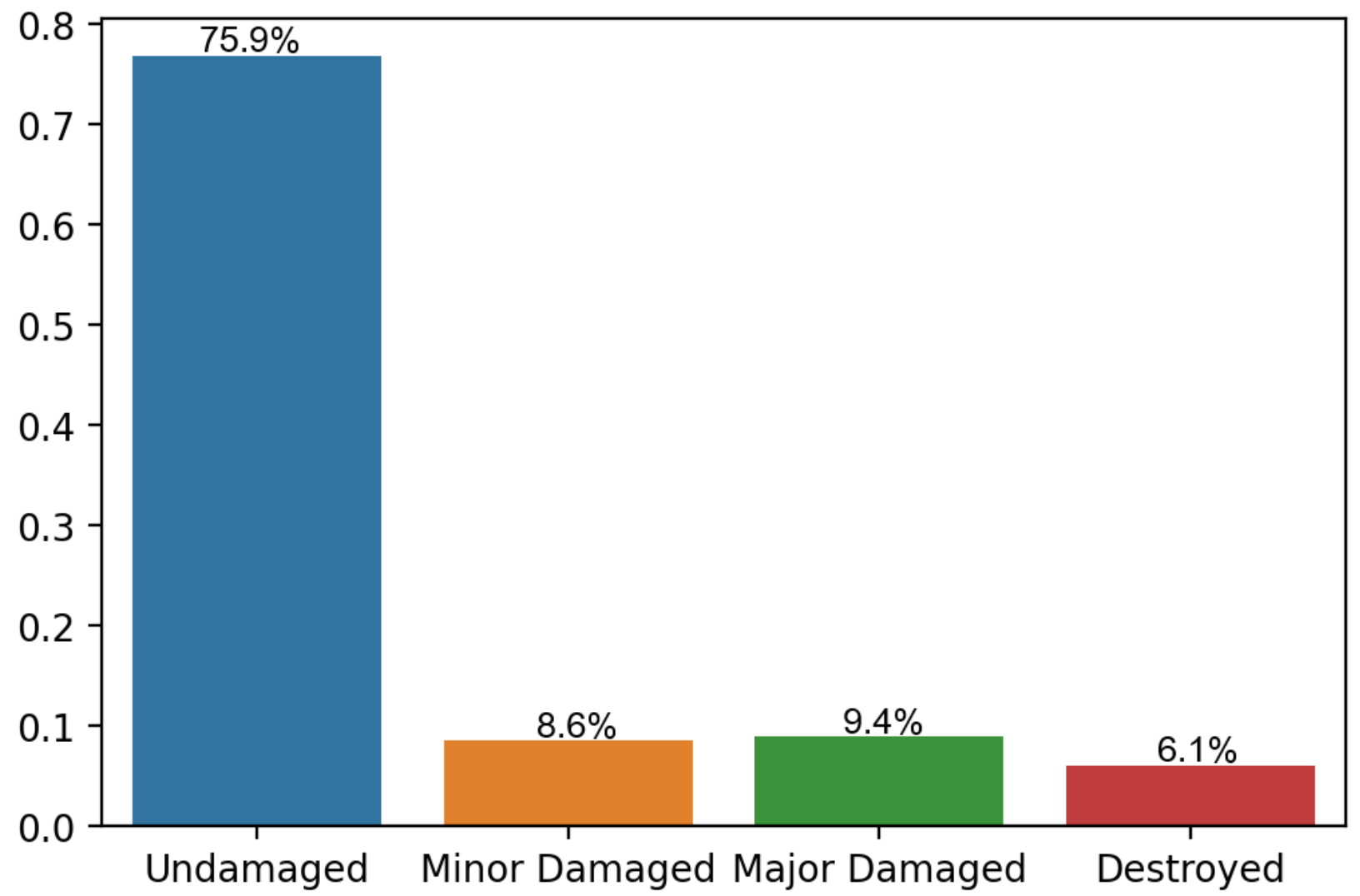
Consistent with real-world disaster case scenarios, the xBD dataset presents severe class imbalance. In terms of the building area/non-building area ratio at the pixel level, the non-building pixel occupies 97% of the image pixels, as shown in Table 1. Regarding the proportional distribution of the damage class at the pixel level, the number of undamaged building pixels far exceeds that of the other three classes, with a ratio of up to 76%. Only 6% of pixels belong to the class of destroyed. The minor-damaged and major-damaged categories account for almost the same proportion. Figure 2 compares the class balance.
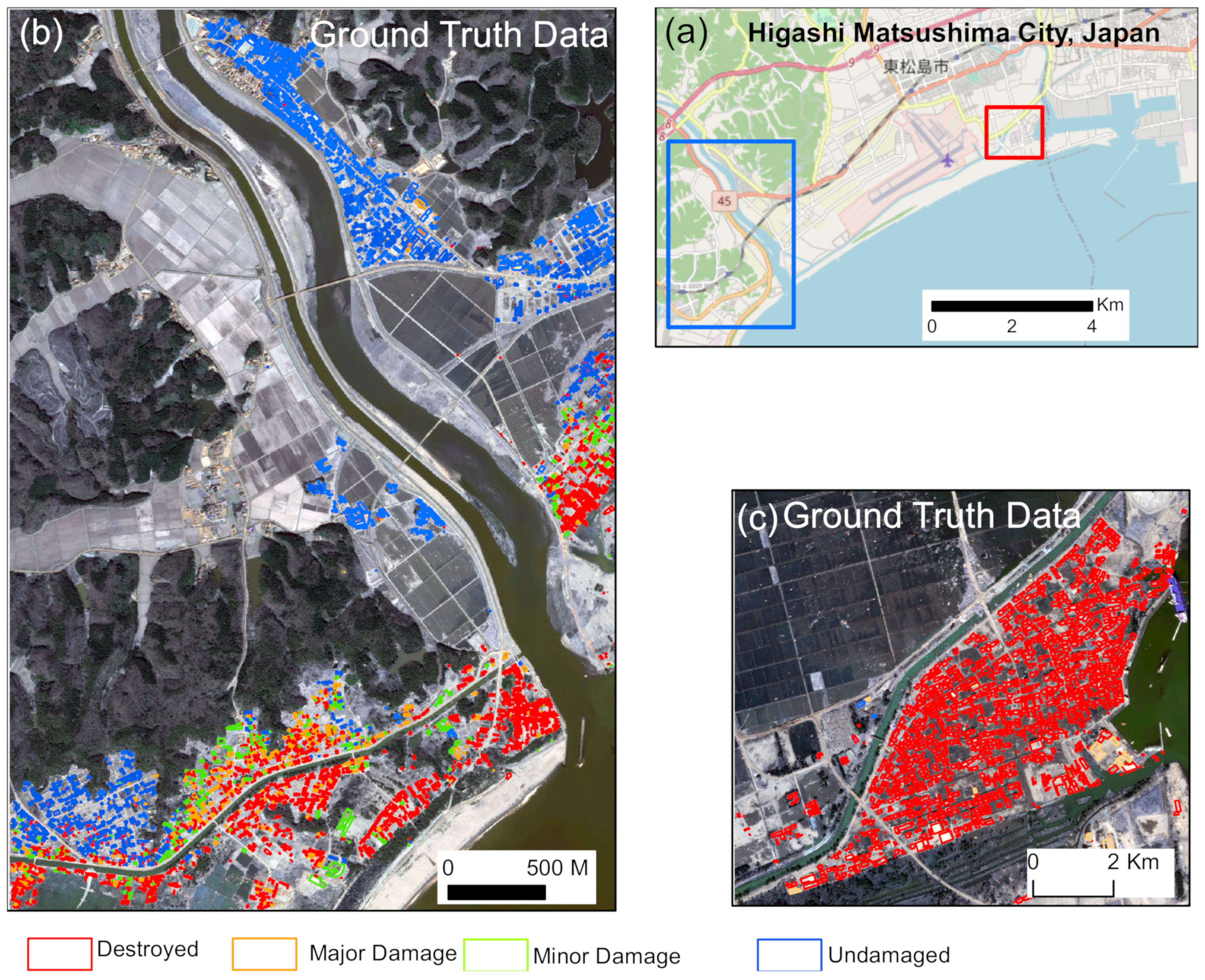
To verify our method’s transferability, we test other satellite imagery with the developed model based on the xBD dataset. Two areas in Higashi Matsushima severely affected by the 2011 Great East Japan Earthquake are used for testing, as shown in Figure 3a–c. These two areas are selected because the xBD dataset does not contain any disaster data from Japan and data on the tsunami in the xBD dataset are scarce. This design can test the ability of our model for to evaluate and predict unknown disasters.
The building damage ground truth data for the testing area are gathered from the field investigation conducted by TTJS [28]. To retain consistency with the xBD data label as much as possible to facilitate the comparative analysis, we recategorize the TTJS building damage data into four classes: “undamaged”, “minor damage” (including “moderate damage and” “minor damage in the” TTJS standard), “major damage,” and “destroyed” (including “washed away,” “collapsed,” and “completely damaged” in the TTJS standard) as shown in Figure 3b,c. We implement this classification standard because standards based on field surveys are much stricter than the visual interpretation based on satellite images.
The four-band multispectral high-resolution Worldview-2 images with a spatial resolution of 0.6 m, collected before and after the 2011 Great East Japan Earthquake, were utilized for validation as shown in background of Figure 3b,c.

3. Methodology

The PPM-SSNet model developed in this research employed dilated convolution, the SE mechanism for attention, and the PPM, as detailed below.

3.1. Dilated Convolution for Large Receptive Fields

Collectively leveraging the global and local features of an input image is effective at solving computer vision problems [29,30,31,32]. Because of the nature of images, the different characters of an image are represented on different scales. A large field in an image includes global appearances such as objects’ contours, whereas a small field includes local appearances such as local textures. This also applies to building localization and damage assessment. One way to realize this idea is with image down-sampling, which reduces the size of an image. This is equivalent to enlarging the receptive field of a convolutional unit in a specific location of an image. Although down-sampling an image leads to less information compared with a reduction in the resolution, it is still used when computing resources (e.g., GPU memory) are limited. Another way to enlarge the convolutional receptive field is by employing dilated convolution [29]. A dilated convolutional unit performs in the same way as normal convolution on an image. The difference is that it has dilated convolutional kernels. A high-dilated rate enables us to have a large convolutional receptive field for the unit. Further, no information is lost with an increasing receptive field under dilated convolution. Figure 4 shows an example of dilated convolution with a dilated rate of 2.

3.2. SE Mechanism for Attention

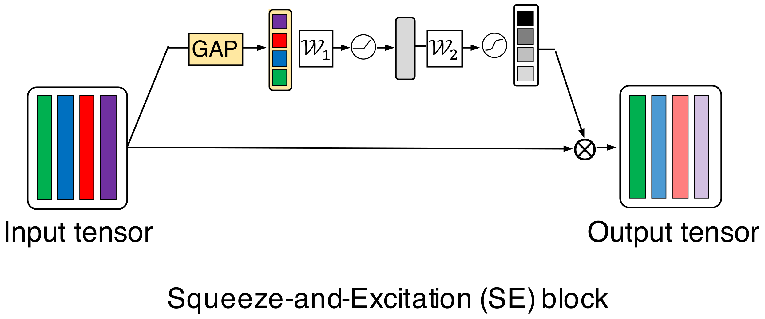
The SE mechanism was originally developed to improve the performance of image classification on ImageNet [33]. It is a weighting system that produces and applies channel-wise weights on a feature map (i.e., the output from an intermediate layer in a CNN). To determine the weight on each channel, it computes the average activation values of the channels; then, these are converted by two linear production layers with ReLU and Sigmoid activation functions to generate the channel-wise weights. The aggregation of the activation values is equivalent to global average pooling, as shown in Figure 5. A CNN, which is equipped with a number of attentional mechanisms, can perform feature recalibration; it learns to selectively emphasize informative features and suppress less useful features, which helps reduce ambiguity when estimating the correct damage level and thus improves the accuracy of building assessment.

3.3. PPM

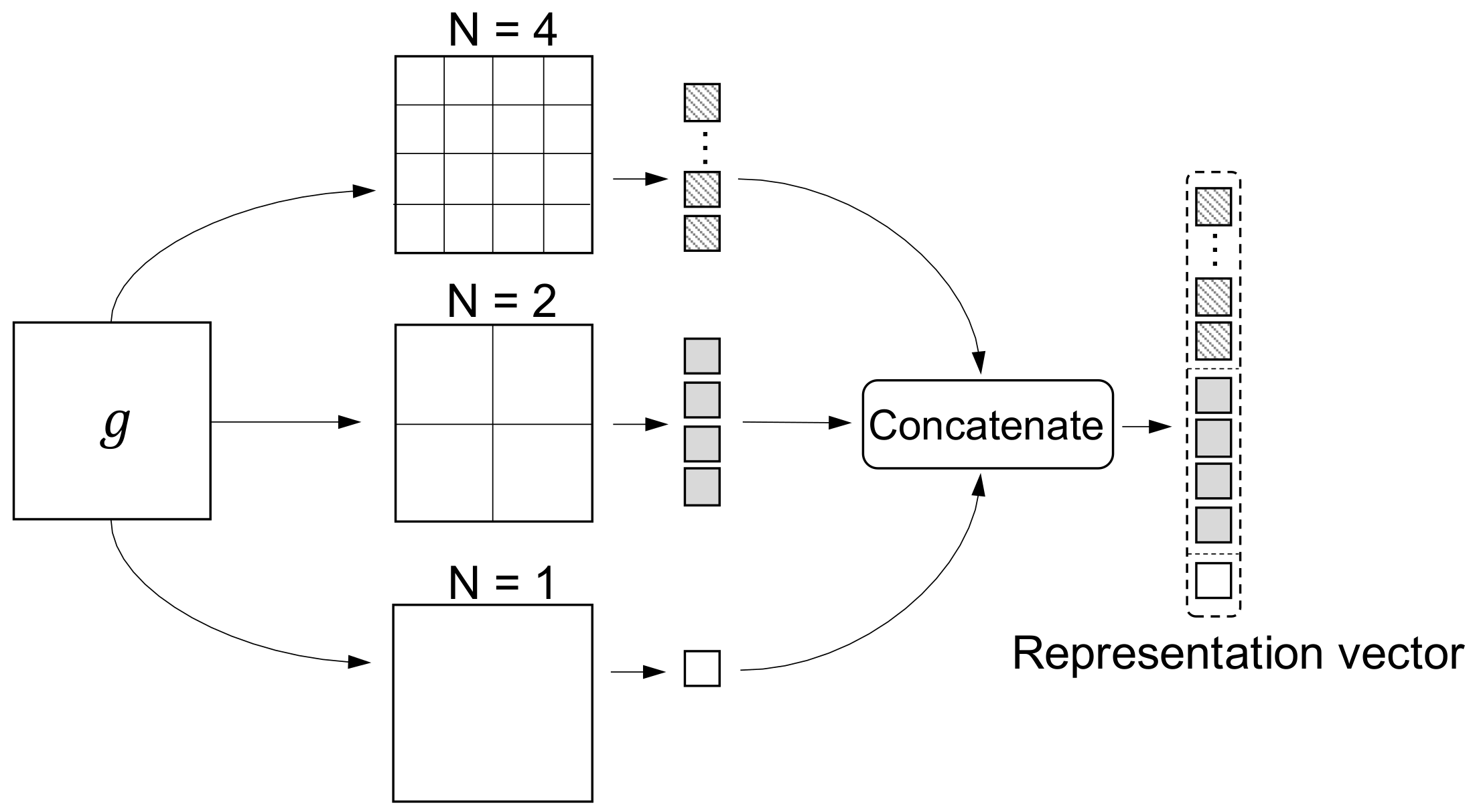
The PPM pools the activation map of each channel in a pyramidal fashion [34]. It makes N × N (N = 1, 2, 4, ...) grids on the activation map of each channel. Each cell of a grid overlaps with a square region of the activation map. Each grid for the channel perfectly covers the whole activation map. On the region covered by each cell of a grid, a user-defined pooling process such as global max pooling or global average pooling is employed to pool the region into a single value. This process quantifies each activation map into a vector with a length equal to N × N. The vectors produced with different N (e.g., 1, 2, and 4) are then concatenated into a representation vector for the channel. The above process is applied to all the channels to produce their representation vectors. The final output of this module is generated by concatenating these representation vectors, as shown in Figure 6. The PPM is a simple yet effective feature aggregation mechanism. It aggregates features from multiple scales. Global features such as the shapes of buildings are covered with a small N (e.g., N = 2), whereas local features such as the details of damaged buildings are covered with a large N (e.g., N = 4). Then, the final output of this mechanism becomes a representative vector of the input sample, which improves the accuracy of building localization and damage assessment.

3.4. Pyramid Pooling Module-Based Semi-Siamese Network (PPM-SSNet)

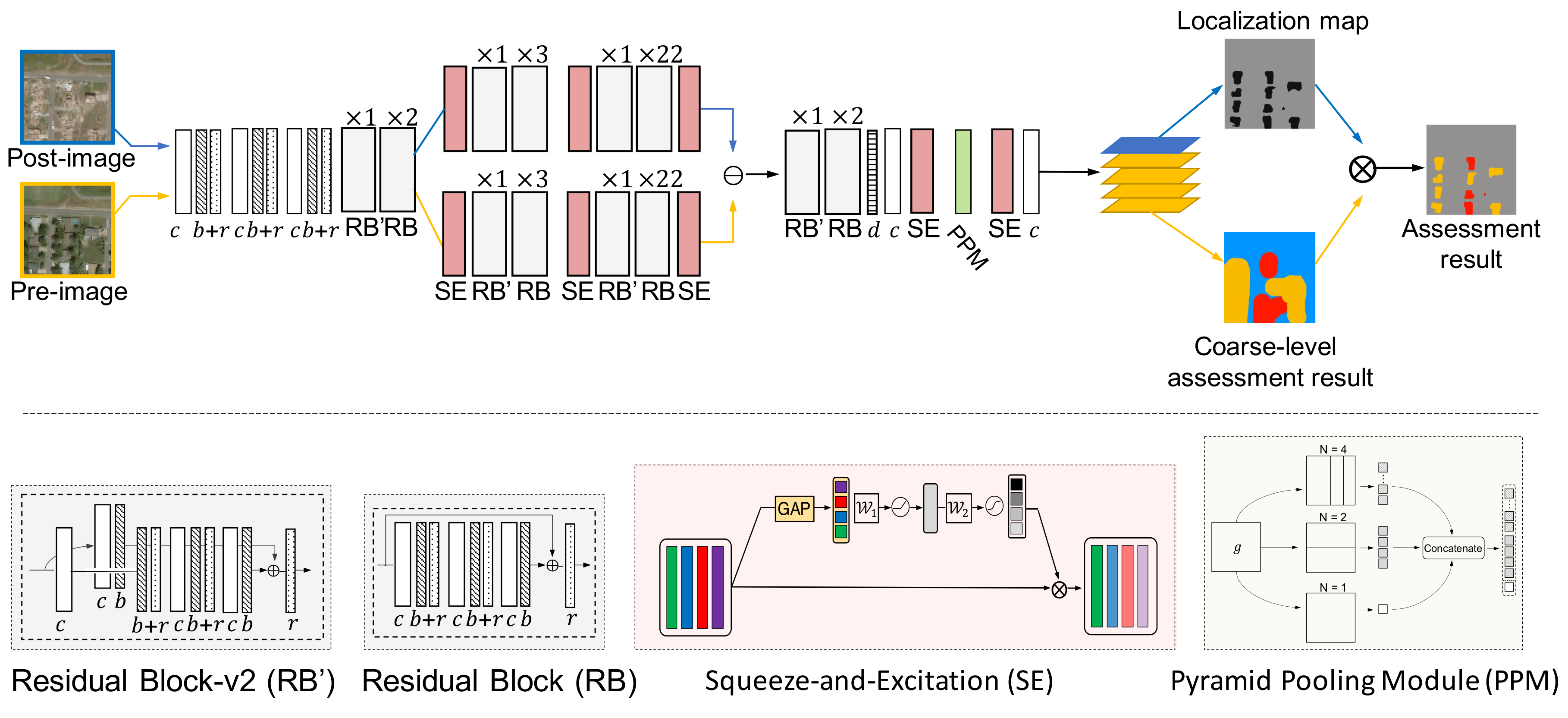
The task of estimating the damage assessment of buildings is divided into two stages. The first stage identifies the buildings on an image. This can be treated as a localization problem in which a system such as a CNN is employed to estimate the binary localization map for an input image. A location with 1 or 0 on the map indicates whether it is a building or not. The localization map is then employed as a prior for the second stage to estimate the damage assessment of a location with a value equal to 1. Based on this idea, we design a network to jointly estimate buildings’ locations and assess their damage. We use the pre-image alone to estimate the location map and then use both the pre- and the post-images to estimate the assessment result. To leverage the localization map to produce an accurate assessment result, we directly multiply it by the output of the assessment estimator. This process corrects the assessment result, improving its quality from a coarse to a fine level (see Figure 7).
Figure 7 shows the architecture. The network is built on a semi-Siamese strategy. We let the weights at the shallow layers of the network share the two input images (i.e., pre-/post-images) to enable it to produce a good “filters’ bank” by collectively learning the low-level features from both. As the layers go deeper, we stop sharing weights and use independent branches for the two inputs instead. The two branches are merged by subtracting one from the other along their channels, which encourages the network to learn the differences between the pre- and post-images. For the tail of the network, we use a single branch of the layers to produce the final estimation result. In the network, we employ RBs with dilated convolution and SE blocks. Our motivation for using RBs is that the network can extract features from large and small receptive fields by employing the large and small dilated rates used in RBs, which may improve its representation ability for the estimations. In addition, SE blocks are employed to encourage the network to focus on the important features, while suppressing the less useful ones. We employ a PPM at the end of the network, immediately before an SE block, and a convolutional layer to aggregate the features.

4. Experimental Analysis

Resampling and data augmentation are adopted in this study. The assessment metrics as well as loss and mask dilation parameter settings are detailed below.

4.1. Resampling

Building damage detection networks based on xBD generally perform badly when detecting minor and major damage, resulting in comparatively low recalls and F1 scores for these two categories because of imbalanced training data. To overcome this problem, we devise several methods to increase the number of minor damage and major damage instances, one of which is over-sampling the training dataset. Since our model is designed to generate pixel-level classification results, we suggest using a main label to decide how many times a picture containing multi-label pixels should be repeated in the training dataset. A weight vector w = ( w 0 , w 1 , w 2 , w 3 ) T is given based on experience, each element of which represents the relative importance of the corresponding category. For picture i, n i is the vector recording the number of pixels of each category and its main label is defined as
Main Label i = arg max j { 0 , 1 , 2 , 3 } w j n i j
where category 0 denotes no damage, category 1 denotes minor damage, and so on. Table 3 shows the main label categories and corresponding repeated times.
Since the images are cropped and randomly augmented later, there is no concern that the repeated pictures are identical to the original ones.
After over-sampling, we perform a cropping-and-selecting process with discrimination. Similar to above, we reweight each pixel as inversely proportional to the frequency of its corresponding damage level. The original image size is 1024 × 1024 . We uniformly sample several 512 × 512 crops from each image and choose the one with the largest sum of pixel weights. Without increasing the volume of the training data, such a process further alleviates the data imbalance of the xBD dataset.

4.2. Data Augmentation

To enhance the generalizability of our model, we apply the following data augmentation methods sequentially to each image. As shown in Table 4, every method is assigned a value, indicating the probability of occurrence. In other words, the sequence of augmentation methods applied to an image is determined randomly and the higher the order, the earlier is the execution.

4.3. Assessment Metrics

End-to-end building damage assessment includes two progressive tasks: building localization and damage classification. The former can be regarded as a binary segmentation, while the latter is a multi-classification task. This study adopts F1 scores, precision, recall, and IoU to evaluate our network’s performance. For the localization task, the F1 score [19] is used:
l o c F 1 = 2 T P l o c 2 T P l o c + F N l o c + F P l o c
where T P l o c denotes the number of pixels precisely categorized as buildings, F N l o c denotes the number of pixels miscategorized as non-building area, and F P l o c represents the number of pixels miscategorized as buildings. For the classification task, the F1 scores, precision, and recall for each damage category are calculated. A macro-IoU is also implemented to quantify accuracy when data are imbalanced:
p r e c i s i o n j = T P j T P j + F P j
r e c a l l j = T P j T P j + F N j
c l s F 1 j = 2 × p r e c i s i o n j × r e c a l l j p r e c i s i o n j + r e c a l l j
I o U j = T P j T P j + F P j + F N j
I o U = 1 4 j = 1 4 I o U j
where j { 0 , 1 , 2 , 3 } , T P j denotes the number of pixels (or instances) precisely categorized as category j, F P j represents the number misclassified as category j, and F N j denotes the number misclassified as other categories [20].

4.4. Loss and Mask Dilation

The output damage scale classification mask has five channels: the four damage levels and no-building label. We adopt a weighted mixed loss that consists of dice loss and focal loss for the damage scale classification loss L d and weighted binary cross-entropy loss for the building segmentation loss L d , which are defined as [20]
L s = [ w s , 1 × y s log P s + w s , 0 × ( 1 y s ) log ( 1 p s ) ]
Seg c = w 1 × Dice c ( m p , m t ) + w 2 × Focal c ( m p , m t )
L d = c = 1 5 w c × Seg c
where y p and y s are the reference label and probability of segmented building, respectively, while m p and m t are the true mask and predicted mask for damage scale c, respectively. As most samples do not contain buildings, we use a bigger weight for the building class, as indicated by w s , 1 in segmentation loss L s . In addition, minor-damaged and-major damaged buildings are uncommon in our samples. Therefore, we select larger weights for them (c = 2, 3) in damage scale classification loss. We also use weighted mixed loss in which focal loss accounts for a larger proportion to improve category imbalance.
To achieve better classification at the boundary, we expand the building damage scale labels. Given the overlap in pixel’ labels, we prioritize minor damaged and major damaged buildings (c = 2, 3), which are relatively vulnerable in the classification.

5. Results and Discussion

5.1. Experimental Setting

In this work, we use PyTorch deep learning framework. All the experimentation and modeling tasks are implemented in the public cluster in the x64 Linux environment with the public computing cloud at the Renmin University of China. This computing cloud is equipped with the Simple Linux Utility for Resource Management (Slurm) scheduling system. Computations are performed on the node titan, which is configured with 128 GB of RAM, two Intel Gold 5218 CPUs, and two NVIDIA Titan RTX GPUs.

5.2. Ablation Study

In this study, we use an ablation experiment to demonstrate the effectiveness of our proposed method. An ablation study typically refers to subtracting a “feature” of the model or algorithm and verifying how this affects performance. Instead of subtracting, however, we gradually add modules such as Siamese, attention, and pyramid pooling into our proposed baseline network to verify its performance. Nevertheless, the improvement of the model performance is incompatible with different sectional tasks. Conducting experiments over several rounds guarantees that the modules of interest boost model performance.
Table 5 and Table 6 show the results of the ablation experiment. The shaded row in the tables represents the performance of our proposed baseline model. The second row in Table 5 indicates that deploying the Siamese network module to the baseline model leads to a significant improvement in all the metrics. Adding the attention module into the model results in a slight decline in all the metrics except the recall rate. The increase in the recall rate might be a consequence of the scale-aware semantic image segmentation that arises with an attention mechanism. We then introduce the PPM, which raises all the metrics except the recall rate slightly. This variation can be attributed to pyramid pooling, which enhances the scale invariance of images, while lowering the risk of over-fitting.
Table 6 shows that sequentially applied modules improve overall performance since total F1, the harmonic mean of the F1 of each category, increases gradually with a mere recession. As for the irregular increment in the metrics, a balance between the precision rate and recall rate and the respective F1s of the different classes often results. For instance, deploying the Siamese network raises F 1 c l f 2 and F 1 c l f 3 and lowers F 1 c l f 0 and F 1 c l f 1 . This is based on the decision boundaries, mutually exclusive in hyperspace, and generated by the recently attached module that changes when another module is consequently applied, leading to fluctuations in the metrics. Finally, the introduction of pyramid pooling, which is noteworthy for its scale-adaptive feature extracting ability, enables the model to yield rather satisfactory metrics for all the categories.
Table 7 also shows the confusion matrix of our final PPM-SSNet. Our model performs well overall and the non-building category holds the highest accuracy of 96.52%; whereas accuracy for the minor damage pixel is only 30.29%.
Table 8 compares the experimental results between the post-and-pre strategy (both pre-disaster and post-disaster images are available) and the post-only strategy (only the post-disaster images are applied). According to the results, the post-only strategy does not perform as well as the pre-and-post strategy, demonstrating the importance of pre-disaster images in building localization and damage classification.

5.3. Comparisons with Other Methods

Since the release of the xBD dataset, some studies have divided a share of its data for training and achieved good results, whereas others use different evaluation metrics to assess accuracy. Moreover, some work is not strictly an end-to-end study, preventing us from being able to compare these published results with ours. To solve this problem, we reproduce previous research results and carry out comparative experiments under uniform experimental conditions. A Mask R-CNN network [19] and Siam-U-Net-Attention network [20] are compared.
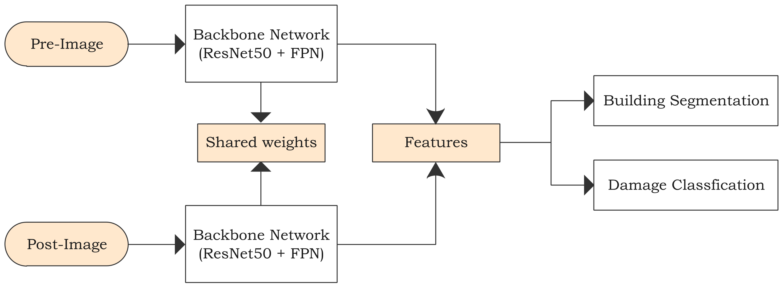
Weber et al. [19] used the Mask R-CNN with the FPN architecture as well as the same model architecture for both building localization and damage classification. However, instead of working with full images, they trained the architecture on both the pre- and the post-image quadrants and fused the final segmentation layer to draw building boundaries more accurately. For the class imbalance problem, they engineered their loss function to weight errors on classes inversely proportional to their occurrence on the dataset. However, this is insufficient to address the problem. In practice, to solve class imbalance, we usually combine multiple approaches such as over-sampling and reweight operation with the weighted loss functions used in our experiment. Figure 8 shows the details of the Mask R-CNN network.
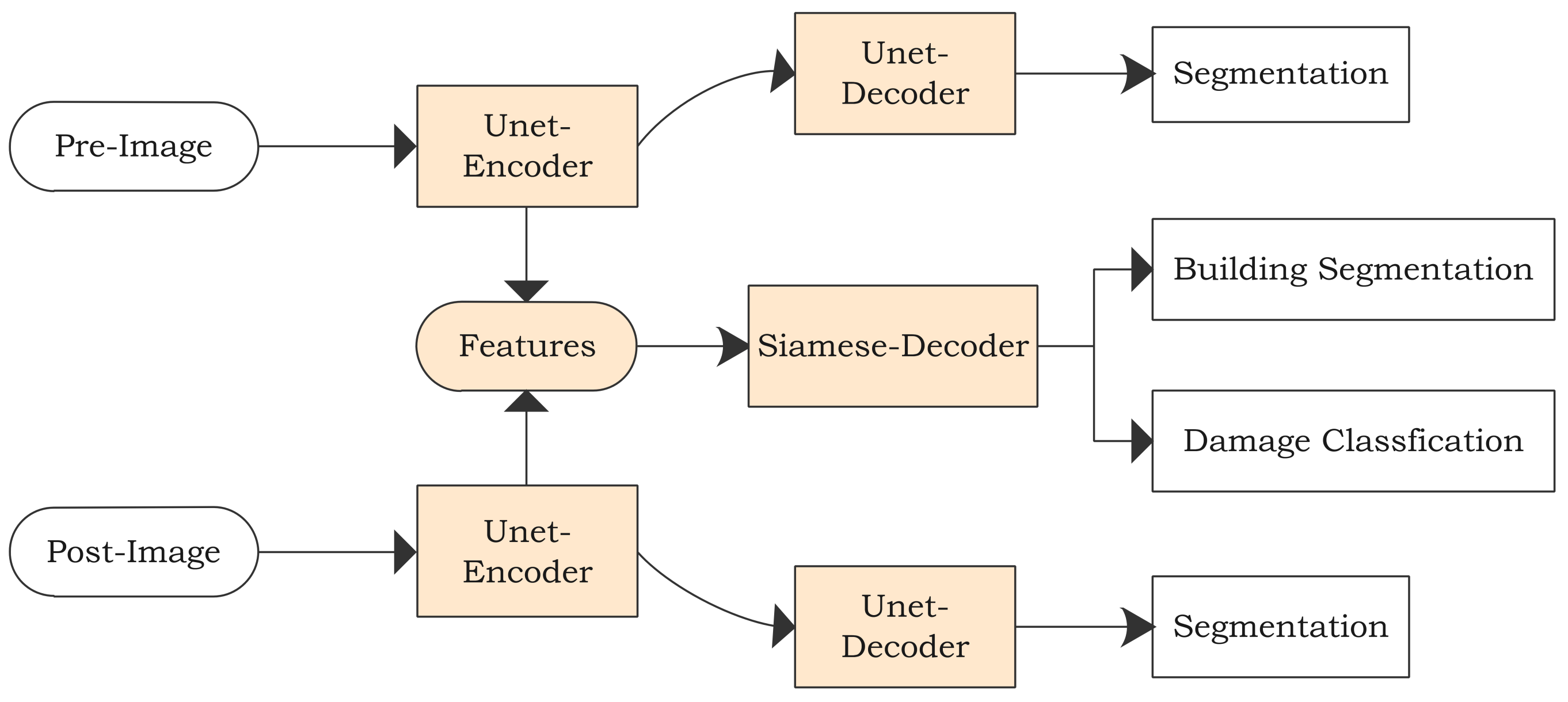
Hao [20] designed an end-to-end Siam-U-Net-Attn model. This model applied U-Net structures to analyze both pre-disaster and post-disaster images and produce the corresponding segmentation masks that showed building locations. Meanwhile, the features extracted from the of the U-Net encoders were utilized in damage classification. More specifically, features produced by both the pre-image and the post-image U-Net encoders would be used by a middle part: a separate decoder in the Siamese network that compared the features from the pre-disaster and the post-disaster frames to detect damage levels. The network achieved an appreciable IoU score on localization and performed well when classifying undamaged and destroyed buildings. However, the model could not identify minor-damaged and major-damaged buildings accurately. Figure 9 shows the structure of the end-to-end Siam-U-Net-Attention network.
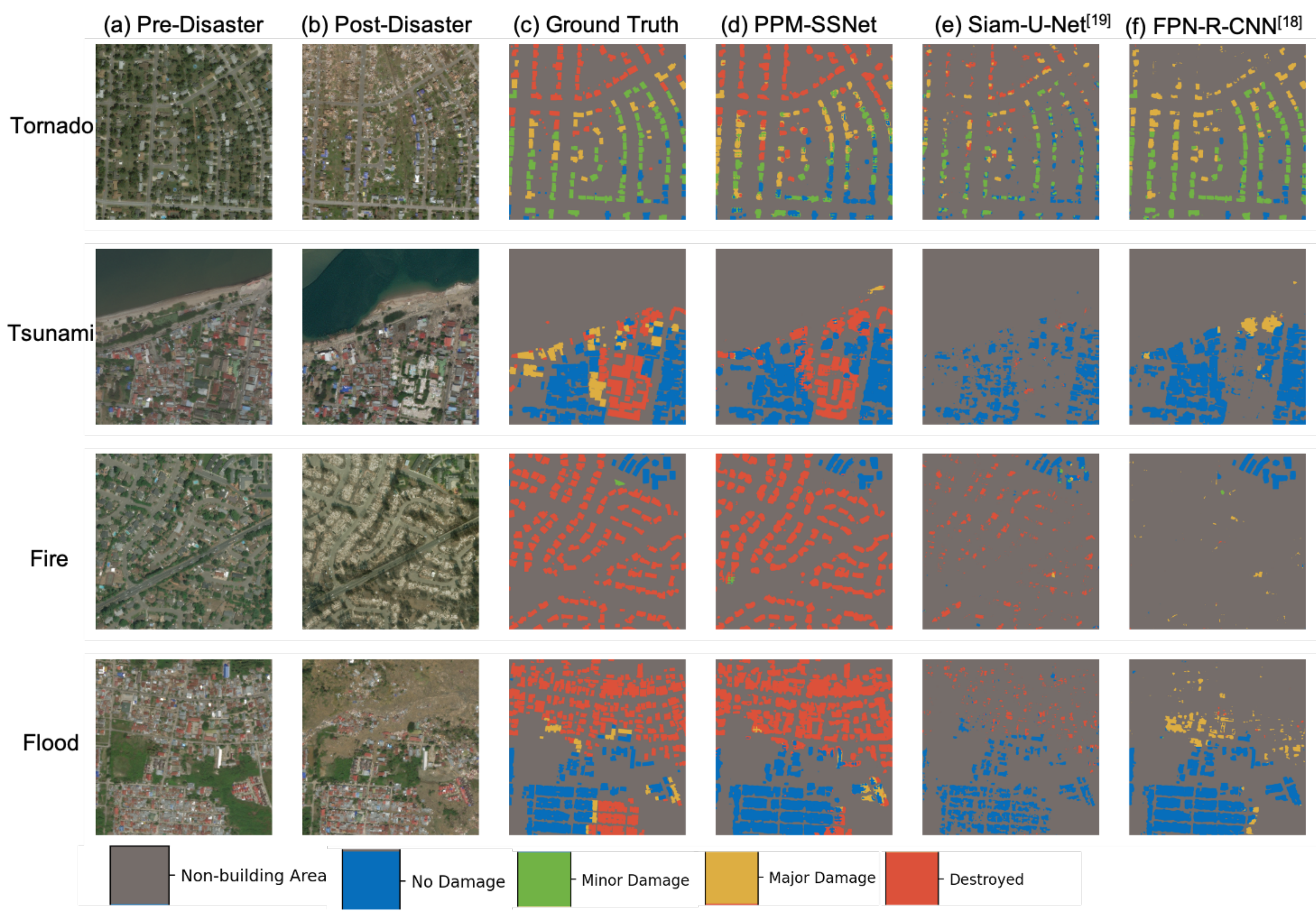
We train and test our network and other methods using the same datasets described above and same parameter settings. The results show that our proposed network easily outperforms the other approaches, as shown in Table 9 and Table 10. We also compare the classification results of earthquakes, tsunamis, floods, typhoons, and volcanic eruptions, as shown in Figure 10. The results again verify the superiority of our method over previous approaches.
Further, our model outperforms baseline models when predicting building localization and damage classification. Post-disaster images with destroyed buildings make a noise to building localization since the edges of destroyed buildings may be vague. FPN-R-CNN classified the majority of destroyed buildings into the no building category, while the U-Net-Siam-Attn’s prediction of destroyed buildings is not robust. In these cases, our model can easily distinguish undamaged and destroyed buildings, but it is difficult to distinguish minor from major damage.

5.4. Robustness of the Method

The validation areas are featured by a various of environmental and geographical background, building structures and spatial settings, tsunami impacts, and satellite image acquisition conditions, as shown in Figure 11(a1,b1,a2,b2), respectively. Considering the differences between validation area and the training data, we approximate the prediction results: When the category of a single pixel matches its neighbor’s, we assume it’s the right prediction(we take a neighbor area of 10*10 pixels).
The predicted results show that the proposed model detects destroyed and undamaged buildings, but separating minor damage from major damage is still challenging, as shown in Figure 11(c1,d1,c2,d2) and Table 11. Partly because the Tohoku tsunami’s annotation standard and that of the xBD dataset are not uniform. The Tohoku tsunami’s building label is from a field survey, while the label of the xBD dataset comes from a visual interpretation, leading to an error in the like-for-like comparison. As the small validation area as shown in Figure 3c contains almost destroyed buildings, therefore we only did quantitative confusion matrix (Table 11) analysis for the larger validation area with variety of damage types as shown in Figure 3b. Still, We can visually interpret that the prediction results of the small validation area as shown in Figure 11(c1) are quite consistent with the ground truth data as shown in Figure 3c. Further, satellite remote sensing is limited when detecting fine-scale building damage because of its lower spatial resolution. Therefore, the method’s inability to distinguish major and minor damage is logical. One way to solve this challenge would be to use high-resolution drone images. In general, our prediction results are consistent with the field observation data.

6. Conclusions

In this study, we developed an end-to-end attention-guided semi-Siamese network with a pyramid-pooling module. Our proposed model yielded satisfactory results when focusing on building localization and damage classification compared with other methods. Employing dilated convolution, the method leveraged the global and local features of an input image. To improve damage classification performance, we adopted a squeeze-and-excitation mechanism, a weighting system that produces and applies channel-wise weights on a feature map. Our ablation experiments on the xBD dataset demonstrated that the developed semi-Siamese network, dilated convolution, and squeeze-and-excitation mechanism were both necessary and effective. Meanwhile, the demonstration with 2011 Great East Japan Earthquake data revealed consistent results with the ground truth data, confirming the effectiveness of evaluating future disasters using our proposed method. Further, it achieved true end-to-end input and output. Thanks to the open source of the large-scale high-precision xBD dataset, which used to be the main challenge of training deep learning models for building damage assessment from satellite imagery, it has become unnecessary to xxxx. Nevertheless, the contribution of this research is developing a damage detection algorithm based on large-scale benchmark data from multiple types of disasters. Therefore, we do not provide targeted solutions for a specific type of disaster.
Our research has some limitations. It is based on the visual information of optical images, meaning that it may be unable to measure extensive flood damage under an intact roof. To address this, researchers could consider using synthetic aperture radar images to detect bottom or sidewall damage [35]. In addition, wall ruptures caused by earthquakes may not be effectively measured, which could be overcome using higher resolution drone images to detect this type of damage [36]. These limitations suggest that despite the contributions of the proposed approach, a highly robust and transplant deep learning model for assessing building damage with high precision is still urgently needed. Since domain shift is still an important challenge in deep learning, satellite imagery is particularly problematic in this field, and this will be the direction of our future efforts.

Author Contributions

Conceptualization, Y.B.; methodology, Y.B., J.H., J.S., X.L.; software, X.H., H.L.; validation, X.H., H.L.; formal analysis, Y.B., J.H., J.S., X.H., H.L., X.L.; investigation, Y.B., E.M., S.K.; resources, Y.B., S.M., E.M., S.K.; data curation, Y.B., E.M., and S.K.; writing—original draft preparation, Y.B., J.H., J.S., X.H., H.L., X.L.; visualization, X.H., H.L.; supervision, Y.B., S.M., X.L., E.M., S.K.; project administration, Y.B., S.M., E.M., S.K.; funding acquisition, Y.B., S.M., E.M., S.K. All authors have read and agreed to the published version of the manuscript.

Funding

This research was partly funded by the Fundamental Research Funds for the Central Universities, Research Funds of Renmin University of China (20XNF022), fund for building world-class universities (disciplines) of Renmin University of China, Major projects of the National Social Science Fund (16ZDA052), Japan Society for the Promotion of Science Kakenhi Program (17H06108), and Core Research Cluster of Disaster Science and Tough Cyberphysical AI Research Center at Tohoku University.

Acknowledgments

This work was supported by the Public Computing Cloud, Renmin University of China. We also thank the SmartData Club, an Entrepreneurship Incubation Team lead by Jinhua Su of Renmin University of China; Wenqi Wu, students from Renmin University of China; and the Core Research Cluster of Disaster Science at Tohoku University (a Designated National University) for their support. We thank the two reviewers for their helpful and constructive comments on our work. The author gratefully acknowledges the support of K.C. Wong Education Foundation, Hong Kong.

Conflicts of Interest

The authors declare no conflict of interest.

Abbreviations

The following abbreviations are used in this manuscript:
PPM-SSNetPyramid Pooling Module-based Semi-Siamese Network
PPMPyramid Pooling Module
CNNConvolutional Neural Network
IoUIntersection over Union
SESqueeze-and-Excitation
RBsResidual Blocks

References

  1. Hillier, J.K.; Matthews, T.; Wilby, R.L.; Murphy, C. Multi-hazard dependencies can increase or decrease risk. Nat. Clim. Chang. 2020, 10, 595–598. [Google Scholar] [CrossRef]
  2. Koshimura, S.; Shuto, N. Response to the 2011 great East Japan earthquake and tsunami disaster. Philos. Trans. R. Soc. A Math. Phys. Eng. Sci. 2015, 373, 20140373. [Google Scholar] [CrossRef] [PubMed] [Green Version]
  3. Mascort-Albea, E.J.; Canivell, J.; Jaramillo-Morilla, A.; Romero-Hernández, R.; Ruiz-Jaramillo, J.; Soriano-Cuesta, C. Action protocols for seismic evaluation of structures and damage restoration of residential buildings in Andalusia (Spain): “IT-Sismo” APP. Buildings 2019, 9, 104. [Google Scholar] [CrossRef] [Green Version]
  4. Mas, E.; Bricker, J.; Kure, S.; Adriano, B.; Yi, C.; Suppasri, A.; Koshimura, S. Field survey report and satellite image interpretation of the 2013 Super Typhoon Haiyan in the Philippines. Nat. Hazards Earth Syst. Sci. 2015, 15, 805–816. [Google Scholar] [CrossRef] [Green Version]
  5. Suppasri, A.; Koshimura, S.; Matsuoka, M.; Gokon, H.; Kamthonkiat, D. Application of remote sensing for tsunami disaster. Remote Sens. Planet Earth 2012, 143–168. [Google Scholar] [CrossRef] [Green Version]
  6. Bai, Y.; Adriano, B.; Mas, E.; Koshimura, S. Building damage assessment in the 2015 Gorkha, Nepal, earthquake using only post-event dual polarization synthetic aperture radar imagery. Earthq. Spectra 2017, 33, 185–195. [Google Scholar] [CrossRef]
  7. Bai, Y.; Gao, C.; Singh, S.; Koch, M.; Adriano, B.; Mas, E.; Koshimura, S. A framework of rapid regional tsunami damage recognition from post-event TerraSAR-X imagery using deep neural networks. IEEE Geosci. Remote Sens. Lett. 2017, 15, 43–47. [Google Scholar] [CrossRef] [Green Version]
  8. Moya, L.; Mas, E.; Koshimura, S. Learning from the 2018 Western Japan Heavy Rains to Detect Floods during the 2019 Hagibis Typhoon. Remote Sens. 2020, 12, 2244. [Google Scholar] [CrossRef]
  9. Koshimura, S.; Moya, L.; Mas, E.; Bai, Y. Tsunami Damage Detection with Remote Sensing: A Review. Geosciences 2020, 10, 177. [Google Scholar] [CrossRef]
  10. Bai, Y.; Mas, E.; Koshimura, S. Towards operational satellite-based damage-mapping using u-net convolutional network: A case study of 2011 tohoku earthquake-tsunami. Remote Sens. 2018, 10, 1626. [Google Scholar] [CrossRef] [Green Version]
  11. Nex, F.; Duarte, D.; Tonolo, F.G.; Kerle, N. Structural building damage detection with deep learning: Assessment of a state-of-the-art cnn in operational conditions. Remote Sens. 2019, 11, 2765. [Google Scholar] [CrossRef] [Green Version]
  12. Xu, J.Z.; Lu, W.; Li, Z.; Khaitan, P.; Zaytseva, V. Building damage detection in satellite imagery using convolutional neural networks. arXiv 2019, arXiv:1910.06444. [Google Scholar]
  13. Rudner, T.G.; Rußwurm, M.; Fil, J.; Pelich, R.; Bischke, B.; Kopačková, V.; Biliński, P. Multi3Net: Segmenting flooded buildings via fusion of multiresolution, multisensor, and multitemporal satellite imagery. In Proceedings of the AAAI Conference on Artificial Intelligence, Honolulu, HI, USA, 27 January–1 February 2019; Volume 33, pp. 702–709. [Google Scholar]
  14. Doshi, J.; Basu, S.; Pang, G. From satellite imagery to disaster insights. arXiv 2018, arXiv:1812.07033. [Google Scholar]
  15. Gupta, R.; Hosfelt, R.; Sajeev, S.; Patel, N.; Goodman, B.; Doshi, J.; Heim, E.; Choset, H.; Gaston, M. xbd: A dataset for assessing building damage from satellite imagery. arXiv 2019, arXiv:1911.09296. [Google Scholar]
  16. Gupta, R.; Goodman, B.; Patel, N.; Hosfelt, R.; Sajeev, S.; Heim, E.; Doshi, J.; Lucas, K.; Choset, H.; Gaston, M. Creating xBD: A Dataset for Assessing Building Damage from Satellite Imagery. In Proceedings of the IEEE/CVF Conference on Computer Vision and Pattern Recognition (CVPR) Workshops, Long Beach, CA, USA, 16–20 June 2019. [Google Scholar]
  17. Gupta, R.; Shah, M. RescueNet: Joint Building Segmentation and Damage Assessment from Satellite Imagery. arXiv 2020, arXiv:2004.07312. [Google Scholar]
  18. Cooner, A.J.; Shao, Y.; Campbell, J.B. Detection of urban damage using remote sensing and machine learning algorithms: Revisiting the 2010 Haiti earthquake. Remote Sens. 2016, 8, 868. [Google Scholar] [CrossRef] [Green Version]
  19. Weber, E.; Kané, H. Building Disaster Damage Assessment in Satellite Imagery with Multi-Temporal Fusion. arXiv 2020, arXiv:2004.05525. [Google Scholar]
  20. Hao, H.; Baireddy, S.; Bartusiak, E.R.; Konz, L.; LaTourette, K.; Gribbons, M.; Chan, M.; Comer, M.L.; Delp, E.J. An Attention-Based System for Damage Assessment Using Satellite Imagery. arXiv 2020, arXiv:2004.05525. [Google Scholar]
  21. Nia, K.R.; Mori, G. Building damage assessment using deep learning and ground-level image data. In Proceedings of the 2017 14th Conference on Computer and Robot Vision (CRV), Edmonton, AB, Canada, 16–19 May 2017; pp. 95–102. [Google Scholar]
  22. Valentijn, T.; Margutti, J.; van den Homberg, M.; Laaksonen, J. Multi-Hazard and Spatial Transferability of a CNN for Automated Building Damage Assessment. Remote Sens. 2020, 12, 2839. [Google Scholar] [CrossRef]
  23. Harirchian, E.; Lahmer, T.; Kumari, V.; Jadhav, K. Application of Support Vector Machine Modeling for the Rapid Seismic Hazard Safety Evaluation of Existing Buildings. Energies 2020, 13, 3340. [Google Scholar] [CrossRef]
  24. Zhuo, G.; Dai, K.; Huang, H.; Li, S.; Shi, X.; Feng, Y.; Li, T.; Dong, X.; Deng, J. Evaluating potential ground subsidence geo-hazard of Xiamen Xiang’an new airport on reclaimed land by SAR interferometry. Sustainability 2020, 12, 6991. [Google Scholar] [CrossRef]
  25. Morfidis, K.E.; Kostinakis, K.G. Use of Artificial Neural Networks in the R/C Buildings’seismic Vulnerabilty Assessment: The Practical Point of View. In Proceedings of the 7th ECCOMAS Thematic Conference on Computational Methods in Structural Dynamics and Earthquake Engineering, Crete, Greece, 24–26 June 2019. [Google Scholar]
  26. Harirchian, E.; Lahmer, T.; Rasulzade, S. Earthquake Hazard Safety Assessment of Existing Buildings Using Optimized Multi-Layer Perceptron Neural Network. Energies 2020, 13, 2060. [Google Scholar] [CrossRef] [Green Version]
  27. Morfidis, K.; Kostinakis, K. Seismic parameters’ combinations for the optimum prediction of the damage state of R/C buildings using neural networks. Adv. Eng. Softw. 2017, 106, 1–16. [Google Scholar] [CrossRef]
  28. Takahashi, T.; Mori, N.; Yasuda, M.; Suzuki, S.; Azuma, K. The 2011 Tohoku Earthquake Tsunami Joint Survey (TTJS) Group. Available online: http://www.coastal.jp/tsunami2011 (accessed on 30 November 2020).
  29. Yu, F.; Koltun, V. Multi-scale context aggregation by dilated convolutions. arXiv 2015, arXiv:1511.07122. [Google Scholar]
  30. Zhang, H.; Patel, V.M. Densely connected pyramid dehazing network. In Proceedings of the IEEE Conference on Computer Vision and Pattern Recognition, Salt Lake City, UT, USA, 18–22 June 2018; pp. 3194–3203. [Google Scholar]
  31. Liu, X.; Suganuma, M.; Sun, Z.; Okatani, T. Dual residual networks leveraging the potential of paired operations for image restoration. In Proceedings of the IEEE Conference on Computer Vision and Pattern Recognition, Long Beach, CA, USA, 16–20 June 2019; pp. 7007–7016. [Google Scholar]
  32. Li, Y.; Song, L.; Chen, Y.; Li, Z.; Zhang, X.; Wang, X.; Sun, J. Learning Dynamic Routing for Semantic Segmentation. In Proceedings of the IEEE/CVF Conference on Computer Vision and Pattern Recognition, Seattle, WA, USA, 16–28 June 2020; pp. 8553–8562. [Google Scholar]
  33. Hu, J.; Shen, L.; Sun, G. Squeeze-and-excitation networks. In Proceedings of the IEEE Conference on Computer Vision and Pattern Recognition, Salt Lake City, UT, USA, 18–22 June 2018; pp. 7132–7141. [Google Scholar]
  34. He, K.; Zhang, X.; Ren, S.; Sun, J. Spatial pyramid pooling in deep convolutional networks for visual recognition. IEEE Trans. Pattern Anal. Mach. Intell. 2015, 37, 1904–1916. [Google Scholar] [CrossRef] [PubMed] [Green Version]
  35. Yamazaki, F.; Iwasaki, Y.; Liu, W.; Nonaka, T.; Sasagawa, T. Detection of damage to building side-walls in the 2011 Tohoku, Japan earthquake using high-resolution TerraSAR-X images. In Proceedings of the Image and Signal Processing for Remote Sensing XIX, Dresden, Germany, 23–26 September 2013; Volume 8892, p. 889212. [Google Scholar]
  36. Duarte, D.; Nex, F.; Kerle, N.; Vosselman, G. Towards a more efficient detection of earthquake induced facade damages using oblique UAV imagery. Int. Arch. Photogramm. Remote Sens. Spat. Inf. Sci. 2017, 42, 93. [Google Scholar] [CrossRef] [Green Version]
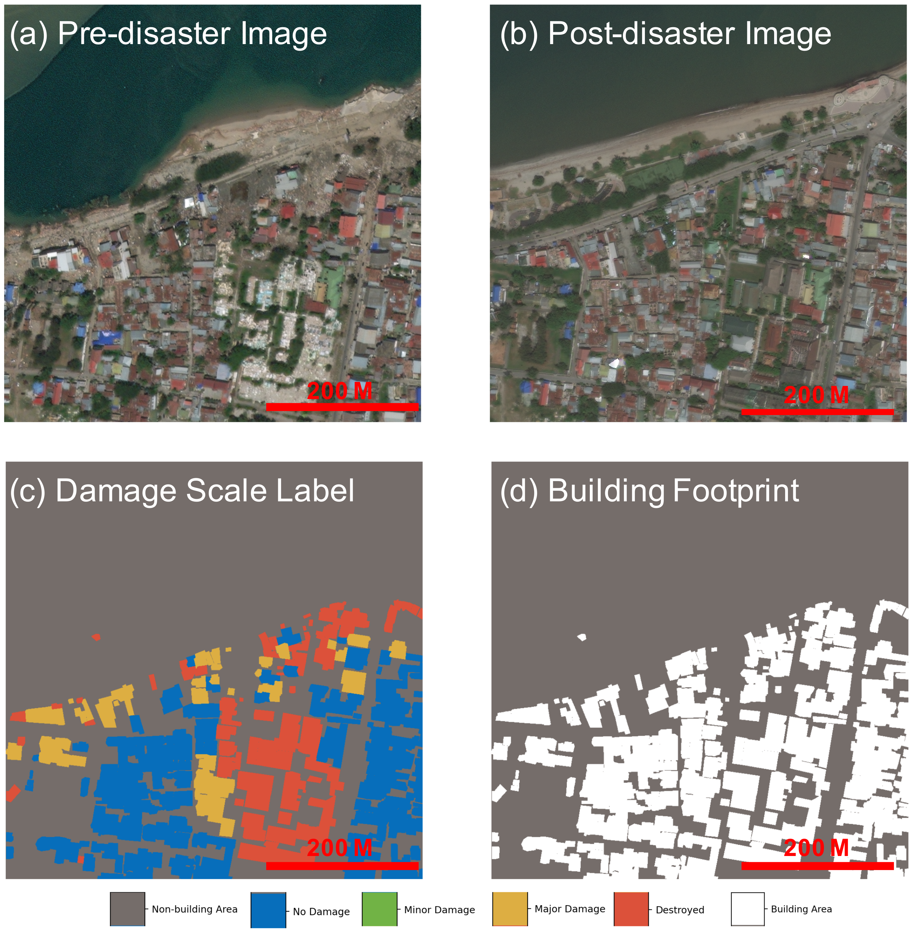
Figure 1. Example of the xBD dataset: Tsunami in Palu, Indonesia. From left to right: (a) Pre-disaster image, (b) Post-disaster image, (c) Damage scale, and (d) Building footprint.
Remotesensing 12 04055 g001
Figure 2. Ratio of damage class at the pixel level.
Remotesensing 12 04055 g002
Figure 3. Validation area. (a) Higashi Matsushima in the Tohoku region of Japan; the rectangular areas marked in blue and red are the selected validation areas; (b) The close-up of the blue area as shown in Figure 10a with the ground truth data of building damage; and (c) The close-up of the red area as shown in Figure 10a with the ground truth data of building damage.
Remotesensing 12 04055 g003
Figure 4. Dilated convolution with dilated rates of 1 (i.e., normal convolution; left side of the figure) and 2 (right side of the figure). g, h, and u mean the input image (or activation map), convolutional kernel, and output. An output u is calculated by summing the multiplications of each value (i, j) at the kernel h and its corresponding value (x, y) at g.
Remotesensing 12 04055 g004
Figure 5. Squeeze-and-excitation (SE) blocks produce and apply channel-wise attention on the activation maps. GAP means global average pooling. w i denotes the ith linear production layer. ReLU and Sigmoid are employed following w 1 and w 2 for the activation functions. The columns depicted in different colors represent the activation map of each channel of the input/output tensor.
Remotesensing 12 04055 g005
Figure 6. The pyramid pooling module (PPM) g represents an activation map of a single channel. N is the number of cells in a row/column of a pooling grid.
Remotesensing 12 04055 g006
Figure 7. The architecture of the proposed network. c, b, d, and r represent the convolutional layer, batch normalization layer, dropout layer, and ReLU layer. SE, RB’, RB, and PPM represent the modules illustrated at the bottom of this figure. The difference between RB’ and RB is that RB’ has an additional convolutional layer + batch normalization layer, which is designed to change the number of channels or size of the input tensor if needed. See Table 2 for more details.
Remotesensing 12 04055 g007
Figure 8. FPN R-CNN network.
Remotesensing 12 04055 g008
Figure 9. Siam-U-Net-Attention network model.
Remotesensing 12 04055 g009
Figure 10. The results from our proposed method and comparisons with others. (a) Image collected before the disaster; (b) Image collected after the disaster; (c) Reference data; (d) Proposed PPM-SSNet model; (e) Siam-U-Net model; and (f) FPN-R-CNN model.
Remotesensing 12 04055 g010
Figure 11. Prediction results from our proposed method in the validation areas. (a1,a2) Pre-disaster image; (b1,b2) Post-disaster image; (c1,c2) Predicted damage scale by the PPM-SSNet model; and (d1,d2) Prediction building footprint by the PPM-SSNet model.
Remotesensing 12 04055 g011
Table 1. Non-building area to building area ratio at the pixel level.
Non-Building AreaBuilding Area
96.97%3.03%
Table 2. Details of the proposed network. Conv., RB’, RB, SE, Drop, and PPM mean the convolutional layer (c), RB-v2 (RB’), RB, SE, dropout layer (d), and PPM (see Figure 7). For the convolutional layer (Conv./conv.), i n , o u t , s t r i d e , and d i l a mean the input’s dimension, output’s dimension, stride, and dilation rate for the layer. k × k means the size of the convolutional kernel. For an SE module, i n , m i d , and o u t mean the input’s dimension, dimension of the output of the middle layer, and output’s dimension. For the PPM, o u t means the output’s dimension.
LayerParametersNumber
Conv. [ 7 × 7 , i n = 3 , o u t = 16 , s t r i d e = 1 , d i l a = 1 ] ×1
ShareConv. [ 3 × 3 , i n = 16 , o u t = 16 , s t r i d e = 1 , d i l a = 1 ] ×1
Conv. [ 3 × 3 , i n = 16 , o u t = 32 , s t r i d e = 2 , d i l a = 1 ] ×1
ShareRB’ conv . , 1 × 1 , i n = 32 , o u t = 64 , s t r i d e = 1 , d i l a = 1 conv . , 3 × 3 , i n = 64 , o u t = 64 , s t r i d e = 2 , d i l a = 1 conv . , 1 × 1 , i n = 64 , o u t = 256 , s t r i d e = 1 , d i l a = 1 down . , 1 × 1 , i n = 32 , o u t = 256 , s t r i d e = 2 , d i l a = 1 ×1
RB conv . , 1 × 1 , i n = 256 , o u t = 64 , s t r i d e = 1 , d i l a = 1 conv . , 3 × 3 , i n = 64 , o u t = 64 , s t r i d e = 1 , d i l a = 1 conv . , 1 × 1 , i n = 64 , o u t = 256 , s t r i d e = 1 , d i l a = 1 ×2
SE [ i n = 256 , m i d = 16 , o u t = 256 ] ×1
RB’ conv . , 1 × 1 , i n = 256 , o u t = 128 , s t r i d e = 1 , d i l a = 1 conv . , 3 × 3 , i n = 128 , o u t = 128 , s t r i d e = 2 , d i l a = 1 conv . , 1 × 1 , i n = 128 , o u t = 512 , s t r i d e = 1 , d i l a = 1 down . , 1 × 1 , i n = 256 , o u t = 512 , s t r i d e = 2 , d i l a = 1 ×1
RB conv . , 1 × 1 , i n = 512 , o u t = 128 , s t r i d e = 1 , d i l a = 1 conv . , 3 × 3 , i n = 128 , o u t = 128 , s t r i d e = 1 , d i l a = 1 conv . , 1 × 1 , i n = 128 , o u t = 512 , s t r i d e = 1 , d i l a = 1 ×3
IndependentSE [ i n = 512 , m i d = 32 , o u t = 512 ] ×1
RB’ conv . , 1 × 1 , i n = 512 , o u t = 256 , s t r i d e = 1 , d i l a = 1 conv . , 3 × 3 , i n = 256 , o u t = 256 , s t r i d e = 1 , d i l a = 2 conv . , 1 × 1 , i n = 256 , o u t = 1024 , s t r i d e = 1 , d i l a = 1 conv . , 1 × 1 , i n = 512 , o u t = 1024 , s t r i d e = 1 , d i l a = 1 ×1
RB conv . , 1 × 1 , i n = 1024 , o u t = 256 , s t r i d e = 1 , d i l a = 1 conv . , 3 × 3 , i n = 256 , o u t = 256 , s t r i d e = 1 , d i l a = 2 conv . , 1 × 1 , i n = 256 , o u t = 1024 , s t r i d e = 1 , d i l a = 1 ×22
SE [ i n = 1024 , m i d = 64 , o u t = 1024 ] ×1
SingleRB’ conv . , 1 × 1 , i n = 1024 , o u t = 512 , s t r i d e = 1 , d i l a = 1 conv . , 3 × 3 , i n = 512 , o u t = 512 , s t r i d e = 1 , d i l a = 4 conv . , 1 × 1 , i n = 512 , o u t = 2048 , s t r i d e = 1 , d i l a = 1 conv . , 1 × 1 , i n = 1024 , o u t = 2048 , s t r i d e = 1 , d i l a = 1 ×1
RB conv . , 1 × 1 , i n = 2048 , o u t = 512 , s t r i d e = 1 , d i l a = 1 conv . , 3 × 3 , i n = 512 , o u t = 512 , s t r i d e = 1 , d i l a = 4 conv . , 1 × 1 , i n = 512 , o u t = 2048 , s t r i d e = 1 , d i l a = 1 ×2
Drop×1
Conv. 3 × 3 , i n = 2048 , o u t = 512 , s t r i d e = 1 , d i l a = 2 ×1
SE [ i n = 512 , m i d = 16 , o u t = 512 ] ×1
SinglePPM [ o u t = 512 ] ×1
SE [ i n = 1024 , m i d = 64 , o u t = 1024 ] ×1
Conv. 1 × 1 , i n = 1024 , o u t = 5 , s t r i d e = 1 , d i l a = 1 ×1
Table 3. Main labels and corresponding repeated times.
Main LabelNo DamageMinor DamageMajor DamageDestroyed
Repeated Times0321
Table 4. Data augmentation methods and probabilities.
MethodPre to PostFlipRotate by 90 DegreeShift Pnt
Probability0.0150.50.950.1
MethodRotationScaleColor shiftsChange hsv
Probability0.10.70.010.01
MethodCLAHEBlurNoiseSaturation
Probability0.00010.00010.00010.0001
MethodBrightnessContrast
Probability0.00010.0001
Table 5. Ablation experiments of the location methods with different modules (the shaded row represents the results of the ablated model).
IOU Non building ( % ) IOU Building ( % ) Mean IoU ( % ) Precision loc ( % ) Recall loc ( % ) F 1 loc ( % ) Dice loc ( % ) Score loc ( % )
Baseline model94.9152.5773.7454.7075.2763.3695.1456.07
+Siamese96.9866.0781.5373.9382.4277.9595.9861.97
+Siamese + Attention96.6065.4581.0364.9887.2674.4996.1560.90
+Siamese + PPM + Attention97.0067.3382.1771.1585.5877.7095.9566.40
Table 6. Ablation experiments of the multi-classification methods with different modules (the shaded row represents the results of the ablated model).
P clf 0 ( % ) R clf 0 ( % ) F 1 clf 0 ( % ) P clf 1 ( % ) R clf 1 ( % ) F 1 clf 1 ( % ) P clf 2 ( % ) R clf 2 ( % ) F 1 clf 2 ( % ) P clf 3 ( % ) R clf 3 ( % ) F 1 clf 3 ( % ) F 1 clf ( % )
Baseline Model87.2293.0490.0454.6426.2035.4348.1456.4151.9585.4145.0258.9652.95
+Siamese90.1979.1084.2822.5955.1432.0567.2465.2566.2392.0755.7369.4455.12
+Siamese + Attention91.3577.2683.7222.5256.6032.2261.7366.6464.1083.0762.3171.2155.08
+Siamese + PPM + Attention90.6489.0789.8535.5149.5041.3665.8064.9365.3687.0857.8969.5561.55
Table 7. Confusion matrix.
Ground Truth
Non-BuildingNo-DamageMinor DamageMajor DamageDestoryed
Non-building 8.88 × 10 8 2.16 × 10 8 2.60 × 10 8 2.84 × 10 8 2.05 × 10 6
No-damage 2.22 × 10 7 3.67 × 10 7 8.31 × 10 5 3.76 × 10 5 7.43 × 10 4
PredictionMinor damage 4.26 × 10 6 2.53 × 10 6 2.06 × 10 6 3.81 × 10 5 1.50 × 10 4
Major damage 4.93 × 10 6 1.60 × 10 6 1.21 × 10 6 4.15 × 10 6 2.06 × 10 5
Destoryed 1.39 × 10 6 4.09 × 10 5 1.12 × 10 5 1.28 × 10 5 1.95 × 10 6
Total 9.20 × 10 8 6.29 × 10 8 6.80 × 10 6 7.91 × 10 6 4.30 × 10 6
Accuracy(%)96.5258.3530.2952.4745.35
Table 8. Comparison between the pre-and-post strategy and the post-only strategy.
Strategy Mean IoU Non building ( % ) Mean IoU Building ( % ) Mean IoU loc ( % ) F 1 loc ( % ) Score loc ( % ) F 1 clf 0 ( % ) F 1 clf 1 ( % ) F 1 clf 2 ( % ) F 1 clf 3 ( % ) F 1 clf ( % )
post-only91.8847.3269.6056.9458.1682.8438.1663.2371.1058.69
pre-and-post97.0067.3382.1777.7066.4089.8541.3665.3669.5561.55
Table 9. Comparison with other methods on the location task.
NetworksMean IOU Non building ( % ) Mean IOU Building ( % ) Mean IoU ( % ) Precision loc ( % ) Recall loc ( % ) F 1 loc ( % )
Siam-U-Net-Diff96.5044.5770.5452.7590.7566.72
Weber et al.95.6348.6272.1385.3082.9084.10
PPM-SSNet97.0067.3382.1771.1585.5877.70
Table 10. Comparison with other methods on the classification task.
Networks P clf 1 ( % ) R clf 1 ( % ) F 1 clf 1 ( % ) P clf 2 ( % ) R clf 2 ( % ) F 1 clf 2 ( % ) P clf 3 ( % ) R clf 3 ( % ) F 1 clf 3 ( % ) P clf 4 ( % ) R clf 4 ( % ) F 1 clf 4 ( % ) F 1 clf ( % )
Siam-U-Net-Diff80.5849.6460.5128.6926.3227.4551.3127.6035.8975.0033.0345.8639.01
Weber et al.94.8056.9071.1058.9022.0032.0070.1038.0049.3089.5040.0360.7148.73
PPM-SSNet90.6489.0789.8535.5149.5041.3665.8064.9365.3687.0857.8969.5561.55
Table 11. Confusion Matrix of Tohoku Tsunami Building Damage Prediction Experiment.
Prediction
Non-BuildingNo-DamageMinor DamageMajor DamageDestoryed
Non-building38,960,37966,36650,87019,19534,488
No-damage215,480368,283862196239,889
Ground TruthMinor damage58,680284134,62917368293
Major damage86,0028433143,6113272
Destoryed196,57980,94212,5506839314,583
Total39,517,120518,080103,24273,343400,525
Accuracy(%)98.5971.0433.5459.4678.54
Publisher’s Note: MDPI stays neutral with regard to jurisdictional claims in published maps and institutional affiliations.