Semantic Segmentation of Sentinel-2 Imagery for Mapping Irrigation Center Pivots


Abstract
1. Introduction
2. Materials and Methods
2.1. Materials
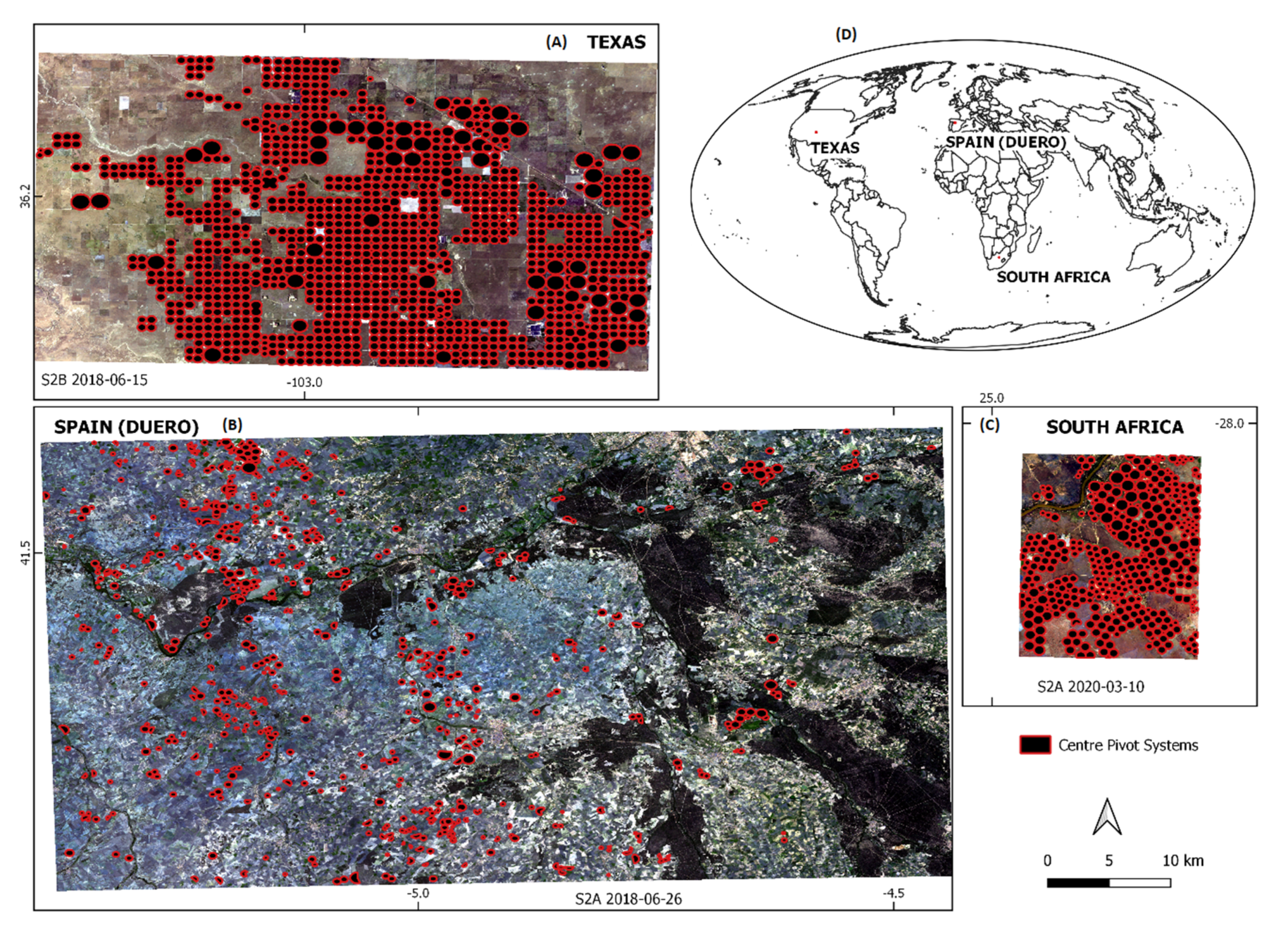
2.1.1. Study Areas
2.1.2. Center Pivot Datasets
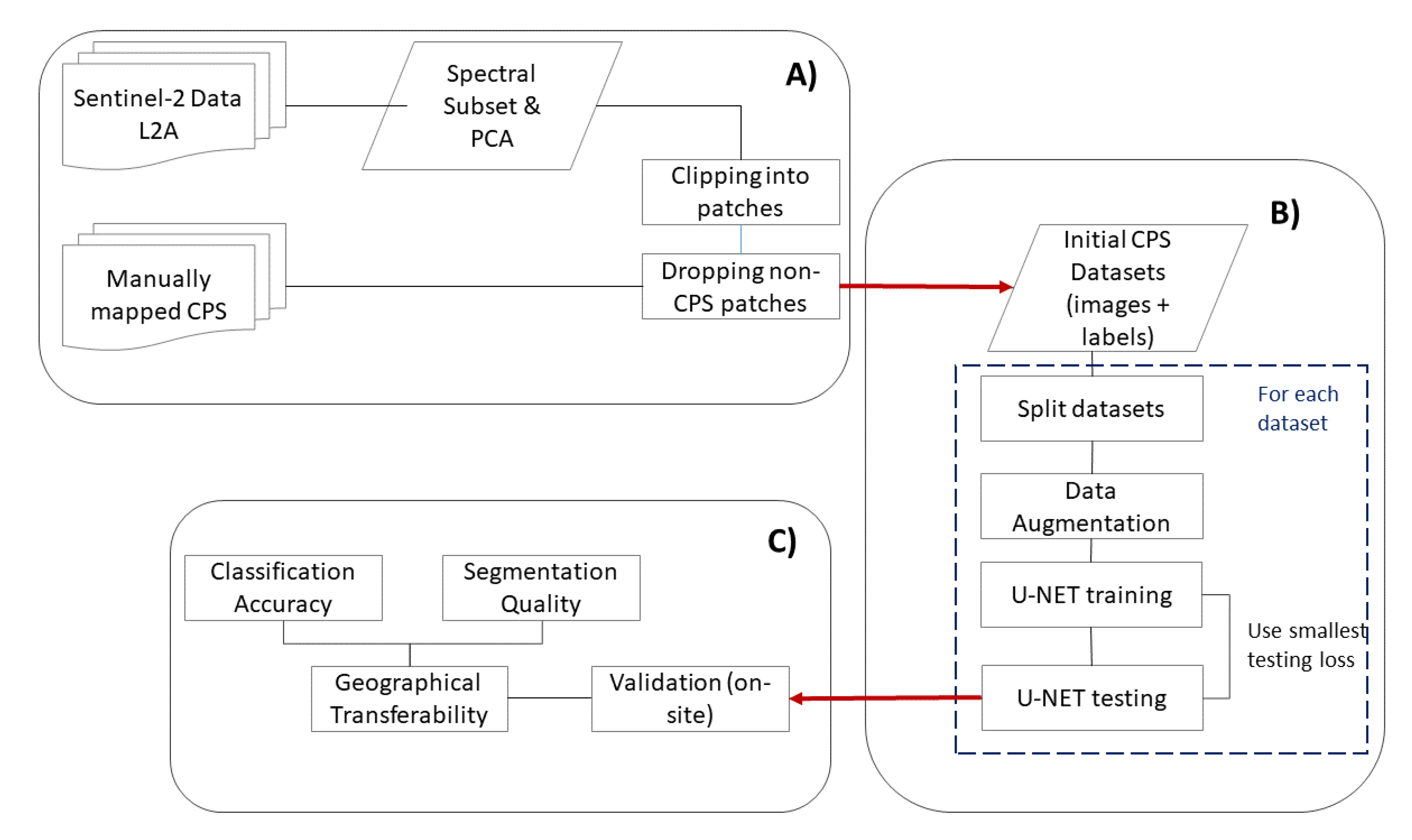
2.2. Methods
2.2.1. Sentinel-2 Data Preparation
- One dataset containing the Sentinel-2 spectral bands 2 (blue), 3 (green), 4 (red), and 5 (NIR1) in accordance to a study undertaken by Saraiva et al. [14], who also used this spectral combination;
- One dataset containing the first three principal components calculated from the nine Sentinel-2 bands available.
2.2.2. Training Data Generation
2.2.3. U-NET Architecture and Training
2.2.4. Validation Strategies
3. Results
3.1. U-NET Training
3.2. Pixel-Based Error Metrics
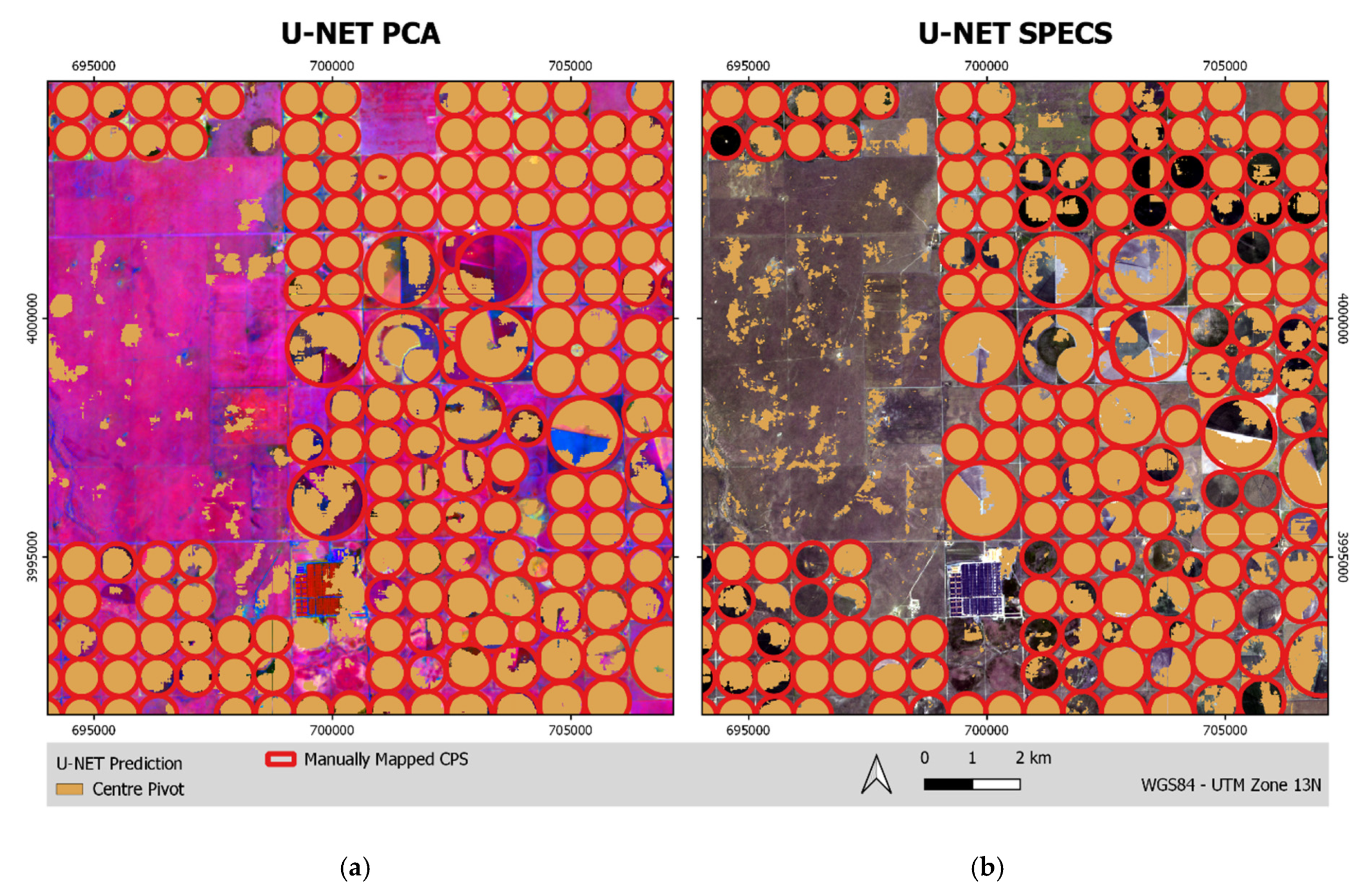
3.3. Segmentation Results
3.3.1. Texas Study Area
3.3.2. Duero Study Area
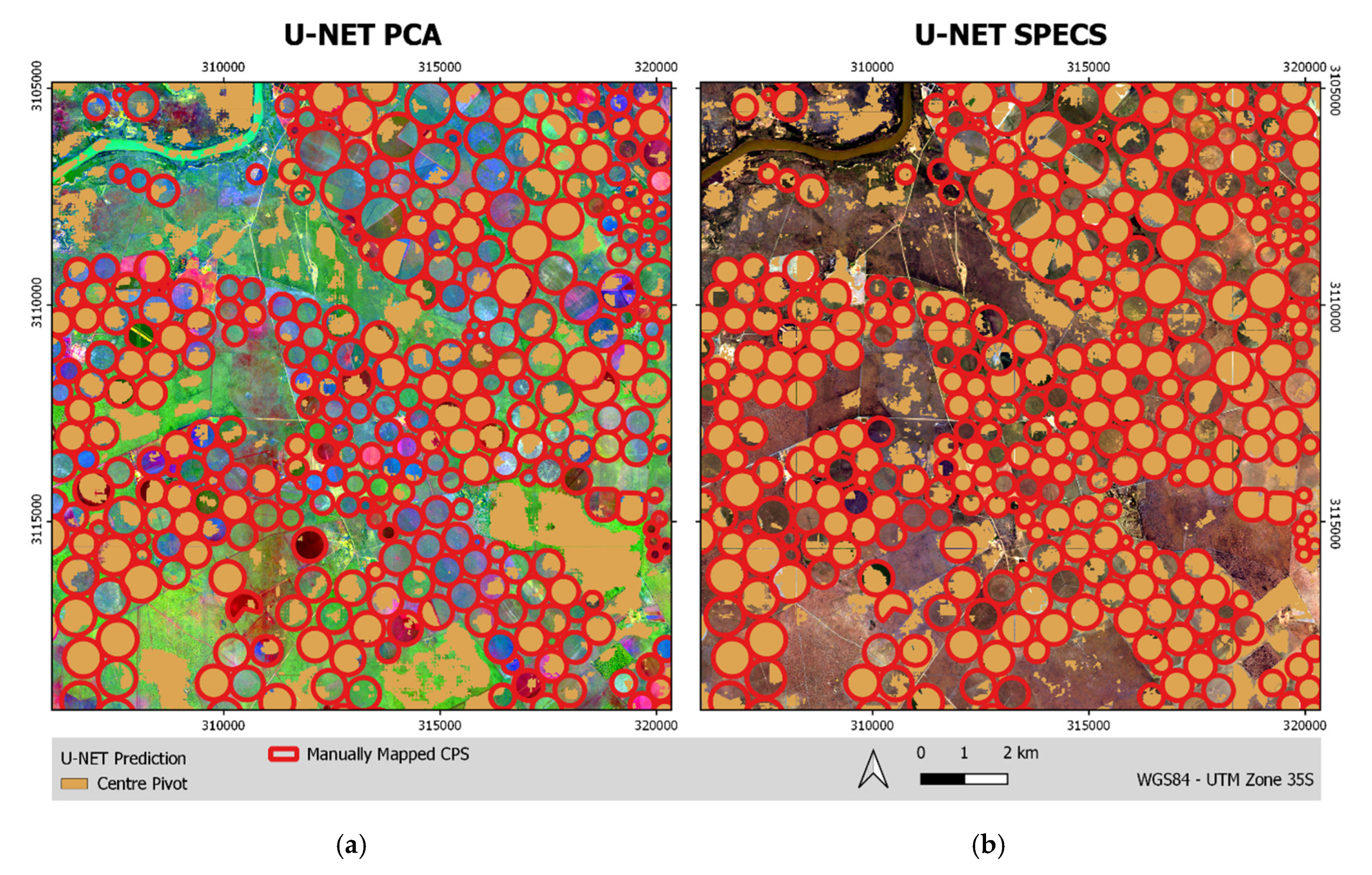
3.3.3. South Africa Study Area
4. Discussion
4.1. Center Pivot Classification and Segmentation
4.2. Geographic Transferability
5. Conclusions
Author Contributions
Funding
Conflicts of Interest
References
- Wisser, D.; Frolking, S.; Douglas, E.M.; Fekete, B.M.; Vörösmarty, C.J.; Schumann, A.H. Global irrigation water demand: Variability and uncertainties arising from agricultural and climate data sets. Geophys. Res. Lett. 2008, 35, 35. [Google Scholar] [CrossRef]
- Hedley, C.; Knox, J.; Raine, S.; Smith, R. Water: Advanced irrigation technologies. In Encyclopedia of Agriculture and Food Systems; Elsevier: Amsterdam, The Netherlands, 2014. [Google Scholar]
- Gilbert, N. Water under pressure: A UN analysis sets out global water-management concerns ahead of Earth Summit. Nature 2012, 483, 256–258. [Google Scholar] [CrossRef]
- De Fraiture, C.; Wichelns, D. Satisfying future water demands for agriculture. Agric. Water Manag. 2010, 97, 502–511. [Google Scholar] [CrossRef]
- Chaturvedi, V.; Hejazi, M.; Edmonds, J.; Clarke, L.; Kyle, P.; Davies, E.; Wise, M. Climate mitigation policy implications for global irrigation water demand. Mitig. Adapt. Strateg. Glob. Chang. 2015, 20, 389–407. [Google Scholar] [CrossRef]
- Flörke, M.; Schneider, C.; McDonald, R.I. Water competition between cities and agriculture driven by climate change and urban growth. Nat. Sustain. 2018, 1, 51–58. [Google Scholar] [CrossRef]
- Geerts, S.; Raes, D. Deficit irrigation as an on-farm strategy to maximize crop water productivity in dry areas. Agric. Water Manag. 2009, 96, 1275–1284. [Google Scholar] [CrossRef]
- Oweis, T.; Pala, M.; Ryan, J. Stabilizing rainfed wheat yields with supplemental irrigation and nitrogen in a Mediterranean climate. Agron. J. 1998, 90, 672–681. [Google Scholar] [CrossRef]
- Kresović, B.; Tapanarova, A.; Tomić, Z.; Životić, L.; Vujović, D.; Sredojević, Z.; Gajić, B. Grain yield and water use efficiency of maize as influenced by different irrigation regimes through sprinkler irrigation under temperate climate. Agric. Water Manag. 2016, 169, 34–43. [Google Scholar] [CrossRef]
- Mueller, N.D.; Gerber, J.S.; Johnston, M.; Ray, D.K.; Ramankutty, N.; Foley, J.A. Closing yield gaps through nutrient and water management. Nature 2012, 490, 254–257. [Google Scholar] [CrossRef] [PubMed]
- McKnight, T.L. Center pivot irrigation in California. Geogr. Rev. 1983, 73, 1–14. [Google Scholar] [CrossRef]
- Abo-Ghobar, H.M. Losses from low-pressure center-pivot irrigation systems in a desert climate as affected by nozzle height. Agric. Water Manag. 1992, 21, 23–32. [Google Scholar] [CrossRef]
- Olivier, F.; Singels, A. Survey of Irrigation Scheduling Practices in the South African Sugar Industry; South African Sugar Technologists’ Association: Durban, South Africa, 2004; Volume 78, pp. 239–244. [Google Scholar]
- Li, J. Increasing crop productivity in an eco-friendly manner by improving sprinkler and micro-irrigation design and management: A review of 20 years’ research at the Iwhr, China. Irrig. Drain. 2018, 67, 97–112. [Google Scholar] [CrossRef]
- Lobo, M., Jr.; Lopes, C.; Silva, W.L.C. Sclerotinia rot losses in processing tomatoes grown under centre pivot irrigation in central Brazil. Plant Pathol. 2000, 49, 51–56. [Google Scholar] [CrossRef]
- Saraiva, M.; Protas, É.; Salgado, M.; Souza, C. Automatic mapping of center pivot irrigation systems from satellite images using deep learning. Remote Sens. 2020, 12, 558. [Google Scholar] [CrossRef]
- Monaghan, J.M.; Daccache, A.; Vickers, L.H.; Hess, T.M.; Weatherhead, E.K.; Grove, I.G.; Knox, J.W. More ‘crop per drop’: Constraints and opportunities for precision irrigation in European agriculture. J. Sci. Food Agric. 2013, 93, 977–980. [Google Scholar] [CrossRef] [PubMed]
- Evans, R.G.; Han, S.; Kroeger, M.; Schneider, S.M. Precision center pivot irrigation for efficient use of water and nitrogen. Precis. Agric. 1996, 75–84. [Google Scholar] [CrossRef]
- Montero, J.; Martínez, A.; Valiente, M.; Moreno, M.A.; Tarjuelo, J.M. Analysis of water application costs with a centre pivot system for irrigation of crops in Spain. Irrig. Sci. 2013, 31, 507–521. [Google Scholar] [CrossRef]
- Dukes, M.D.; Perry, C. Uniformity testing of variable-rate center pivot irrigation control systems. Precis. Agric. 2006, 7, 205. [Google Scholar] [CrossRef]
- Carlson, M.P. The Nebraska Center-Pivot Inventory: An example of operational satellite remote sensing on a long-term basis. Photogramm. Eng. Remote Sens. 1989, 55, 587–590. [Google Scholar]
- Zhang, C.; Yue, P.; Di, L.; Wu, Z. automatic identification of center pivot irrigation systems from landsat images using convolutional neural networks. Agriculture 2018, 8, 147. [Google Scholar] [CrossRef]
- Ronneberger, O.; Fischer, P.; Brox, T. U-Net: Convolutional networks for biomedical image segmentation. In Lecture Notes in Computer Science, Proceedings of the Medical Image Computing and Computer-Assisted Intervention—MICCAI, Munich, Germany, 5–9 October 2015; Navab, N., Hornegger, J., Wells, W.M., Frangi, A.F., Eds.; Springer International Publishing: Cham, Switzerland, 2015; pp. 234–241. [Google Scholar]
- Shelhamer, E.; Long, J.; Darrell, T. Fully convolutional networks for semantic segmentation. IEEE Trans. Pattern Anal. Mach. Intell. 2017, 39, 640–651. [Google Scholar] [CrossRef] [PubMed]
- Zhu, X.X.; Tuia, D.; Mou, L.; Xia, G.-S.; Zhang, L.; Xu, F.; Fraundorfer, F. Deep learning in remote sensing: A comprehensive review and list of resources. IEEE Geosci. Remote Sens. Mag. 2017, 5, 8–36. [Google Scholar] [CrossRef]
- Ghosh, A.; Ehrlich, M.; Shah, S.; Davis, L.; Chellappa, R. Stacked U-Nets for ground material segmentation in remote sensing imagery. In Proceedings of the 2018 IEEE/CVF Conference on Computer Vision and Pattern Recognition Workshops (CVPRW), Salt Lake City, UT, USA, 18–22 June 2018; pp. 252–2524. [Google Scholar]
- Zhao, X.; Yuan, Y.; Song, M.; Ding, Y.; Lin, F.; Liang, D.; Zhang, D. Use of unmanned aerial vehicle imagery and deep learning unet to extract rice lodging. Sensors 2019, 19, 3859. [Google Scholar] [CrossRef] [PubMed]
- Frampton, W.J.; Dash, J.; Watmough, G.; Milton, E.J. Evaluating the capabilities of Sentinel-2 for quantitative estimation of biophysical variables in vegetation. ISPRS J. Photogramm. Remote Sens. 2013, 82, 83–92. [Google Scholar] [CrossRef]
- Singh, A.; Harrison, A. Standardized principal components. Int. J. Remote Sens. 1985, 6, 883–896. [Google Scholar] [CrossRef]
- Stephenson, N. Actual evapotranspiration and deficit: Biologically meaningful correlates of vegetation distribution across spatial scales. J. Biogeogr. 1998, 25, 855–870. [Google Scholar] [CrossRef]
- Johnston, C.A. Agricultural expansion: Land use shell game in the U.S. Northern Plains. Landsc. Ecol. 2014, 29, 81–95. [Google Scholar] [CrossRef]
- Crosbie, R.S.; Scanlon, B.R.; Mpelasoka, F.S.; Reedy, R.C.; Gates, J.B.; Zhang, L. Potential climate change effects on groundwater recharge in the High Plains Aquifer, USA. Water Resour. Res. 2013, 49, 3936–3951. [Google Scholar] [CrossRef]
- Terrell, B.L.; Johnson, P.N.; Segarra, E. Ogallala aquifer depletion: Economic impact on the Texas high plains. Water Policy 2002, 4, 33–46. [Google Scholar] [CrossRef]
- Nativ, R.; Smith, D.A. Hydrogeology and geochemistry of the Ogallala aquifer, Southern High Plains. J. Hydrol. 1987, 91, 217–253. [Google Scholar] [CrossRef]
- Johnson, J.; Johnson, P.N.; Segarra, E.; Willis, D. Water conservation policy alternatives for the Ogallala Aquifer in Texas. Water Policy 2009, 11, 537–552. [Google Scholar] [CrossRef]
- Mayor, B.; López-Gunn, E.; Villarroya, F.I.; Montero, E. Application of a water–energy–food nexus framework for the Duero river basin in Spain. Water Int. 2015, 40, 791–808. [Google Scholar] [CrossRef]
- Segovia-Cardozo, D.A.; Rodriguez-Sinobas, L.; Zubelzu, S. Water use efficiency of corn among the irrigation districts across the Duero river basin (Spain): Estimation of local crop coefficients by satellite images. Agric. Water Manag. 2019, 212, 241–251. [Google Scholar] [CrossRef]
- Miguel, Á.D.; Kallache, M.; García-Calvo, E. The water footprint of agriculture in Duero river basin. Sustainability 2015, 7, 6759–6780. [Google Scholar] [CrossRef]
- Lopez-Gunn, E.; Zorrilla, P.; Prieto, F.; Llamas, M.R. Lost in translation? Water efficiency in Spanish agriculture. Agric. Water Manag. 2012, 108, 83–95. [Google Scholar] [CrossRef]
- Ceballos, A.; Martinez-Fernandez, J.; Luengo-Ugidos, M.A. Analysis of rainfall trends and dry periods on a pluviometric gradient representative of Mediterranean climate in the Duero Basin, Spain. J. Arid Environ. 2004, 58, 215–233. [Google Scholar] [CrossRef]
- Gil, M.; Garrido, A.; Gómez-Ramos, A. Economic analysis of drought risk: An application for irrigated agriculture in Spain. Agric. Water Manag. 2011, 98, 823–833. [Google Scholar] [CrossRef]
- Bischoff-Mattson, Z.; Maree, G.; Vogel, C.; Lynch, A.; Olivier, D.; Terblanche, D. Shape of a water crisis: Practitioner perspectives on urban water scarcity and ‘Day Zero’ in South Africa. Water Policy 2020, 22, 193–210. [Google Scholar] [CrossRef]
- Rusere, F.; Crespo, O.; Dicks, L.; Mkuhlani, S.; Francis, J.; Zhou, L. Enabling acceptance and use of ecological intensification options through engaging smallholder farmers in semi-arid rural Limpopo and Eastern Cape, South Africa. Agroecol. Sustain. Food Syst. 2020, 44, 696–725. [Google Scholar] [CrossRef]
- Perret, S.R. Water policies and smallholding irrigation schemes in South Africa: A history and new institutional challenges. Water Policy 2002, 4, 283–300. [Google Scholar] [CrossRef]
- Du Plessis, A. Water scarcity and other significant challenges for South Africa. In Freshwater Challenges of South Africa and its Upper Vaal River: Current State and Outlook; du Plessis, A., Ed.; Springer International Publishing: Cham, Switzerland, 2017; pp. 119–125. ISBN 978-3-319-49502-6. [Google Scholar]
- Elum, Z.A.; Modise, D.M.; Marr, A. Farmer’s perception of climate change and responsive strategies in three selected provinces of South Africa. Clim. Risk Manag. 2017, 16, 246–257. [Google Scholar] [CrossRef]
- MacEachren, A.M. Compactness of geographic shape: Comparison and evaluation of measures. Geogr. Ann. Ser. B Hum. Geogr. 1985, 67, 53–67. [Google Scholar] [CrossRef]
- Drusch, M.; Del Bello, U.; Carlier, S.; Colin, O.; Fernandez, V.; Gascon, F.; Hoersch, B.; Isola, C.; Laberinti, P.; Martimort, P. Sentinel-2: ESA’s optical high-resolution mission for GMES operational services. Remote Sens. Environ. 2012, 120, 25–36. [Google Scholar] [CrossRef]
- Richter, K.; Hank, T.B.; Vuolo, F.; Mauser, W.; D’Urso, G. Optimal exploitation of the Sentinel-2 spectral capabilities for crop leaf area index mapping. Remote Sens. 2012, 4, 561–582. [Google Scholar] [CrossRef]
- Berk, A.; Anderson, G.P.; Bernstein, L.S.; Acharya, P.K.; Dothe, H.; Matthew, M.W.; Adler-Golden, S.M.; Chetwynd, J.H.; Richtsmeier, S.C.; Pukall, B.; et al. MODTRAN4 radiative transfer modeling for atmospheric correction. In Proceedings of the SPIE’s International Symposium on Optical Science, Engineering, and Instrumentation, Denver, CO, USA, 20 October 1999; Volume 3756, pp. 348–353. [Google Scholar] [CrossRef]
- Verhoef, W.; Bach, H. Simulation of hyperspectral and directional radiance images using coupled biophysical and atmospheric radiative transfer models. Remote Sens. Environ. 2003, 87, 23–41. [Google Scholar] [CrossRef]
- Clevers, J.G.P.W.; Gitelson, A.A. Remote estimation of crop and grass chlorophyll and nitrogen content using red-edge bands on Sentinel-2 and-3. Int. J. Appl. Earth Obs. Geoinf. 2013, 23, 344–351. [Google Scholar] [CrossRef]
- Pearson, K. Principal components analysis. Lond. Edinb. Dublin Philos. Mag. J. Sci. 1901, 6, 559. [Google Scholar] [CrossRef]
- Byrne, G.; Crapper, P.; Mayo, K. Monitoring land-cover change by principal component analysis of multitemporal Landsat data. Remote Sens. Environ. 1980, 10, 175–184. [Google Scholar] [CrossRef]
- Cablk, M.; Minor, T. Detecting and discriminating impervious cover with high-resolution IKONOS data using principal component analysis and morphological operators. Int. J. Remote Sens. 2003, 24, 4627–4645. [Google Scholar] [CrossRef]
- Celik, T. Unsupervised change detection in satellite images using principal component analysis and k-means clustering. IEEE Geosci. Remote Sens. Lett. 2009, 6, 772–776. [Google Scholar] [CrossRef]
- Hotelling, H. Analysis of a complex of statistical variables into principal components. J. Educ. Psychol. 1933, 24, 417. [Google Scholar] [CrossRef]
- Xu, Y.; Xiao, T.; Zhang, J.; Yang, K.; Zhang, Z. Scale-invariant convolutional neural networks. arXiv 2014, arXiv:1411.6369. [Google Scholar]
- Marcos, D.; Volpi, M.; Tuia, D. Learning rotation invariant convolutional filters for texture classification. In Proceedings of the 23rd International Conference on Pattern Recognition (ICPR), Cancun, Mexico, 4–8 December 2016; pp. 2012–2017. [Google Scholar]
- Akeret, J.; Chang, C.; Lucchi, A.; Refregier, A. Radio frequency interference mitigation using deep convolutional neural networks. Astron. Comput. 2017, 18, 35–39. [Google Scholar] [CrossRef]
- LeCun, Y.; Bottou, L.; Bengio, Y.; Haffner, P. Gradient-based learning applied to document recognition. Proc. IEEE 1998, 86, 2278–2324. [Google Scholar] [CrossRef]
- Dahl, G.E.; Sainath, T.N.; Hinton, G.E. Improving deep neural networks for LVCSR using rectified linear units and dropout. In Proceedings of the IEEE International Conference on Acoustics, Speech and Signal Processing, Vancouver, BC, Canada, 26–31 May 2013; pp. 8609–8613. [Google Scholar]
- Kingma, D.P.; Ba, J. Adam: A method for stochastic optimization. In Proceedings of the 3rd International Conference for Learning Representations, San Diego, CA, USA, 7–9 May 2015. [Google Scholar]
- Wu, H.; Gu, X. Towards dropout training for convolutional neural networks. Neural Netw. 2015, 71, 1–10. [Google Scholar] [CrossRef]
- Sokolova, M.; Lapalme, G. A systematic analysis of performance measures for classification tasks. Inf. Process. Manag. 2009, 45, 427–437. [Google Scholar] [CrossRef]
- Kohl, M. Performance measures in binary classification. Int. J. Stat. Med. Res. 2012, 1, 79–81. [Google Scholar] [CrossRef]
- Decker, L.R.; Pollack, I. Confidence ratings, message-reception, and the receiver operator characteristic. J. Acoust. Soc Am. 1957, 29, 1263. [Google Scholar] [CrossRef]
- Hanley, J.A.; McNeil, B.J. The meaning and use of the area under a receiver operating characteristic (ROC) curve. Radiology 1982, 143, 29–36. [Google Scholar] [CrossRef]
- Hossin, M.; Sulaiman, M. A review on evaluation metrics for data classification evaluations. Int. J. Data Min. Knowl. Manag. Process 2015, 5, 1. [Google Scholar]
- Tharwat, A. Classification assessment methods. Appl. Comput. Inform. 2020. [Google Scholar] [CrossRef]
- López, J.; Torres, D.; Santos, S.; Atzberger, C. Spectral imagery tensor decomposition for semantic segmentation of remote sensing data through fully convolutional networks. Remote Sens. 2020, 12, 517. [Google Scholar] [CrossRef]
- Wertheimer, M. A brief introduction to gestalt, identifying key theories and principles. Psychol. Forsch. 1923, 4, 301–350. [Google Scholar] [CrossRef]
- Lang, S. Object-based image analysis for remote sensing applications: Modeling reality—Dealing with complexity. In Object-Based Image Analysis: Spatial Concepts for Knowledge-Driven Remote Sensing Applications; Blaschke, T., Lang, S., Hay, G.J., Eds.; Springer: Berlin/Heidelberg, Germany, 2008; pp. 3–27. ISBN 978-3-540-77058-9. [Google Scholar]
- Li, R.; Liu, W.; Yang, L.; Sun, S.; Hu, W.; Zhang, F.; Li, W. Deepunet: A deep fully convolutional network for pixel-level sea-land segmentation. IEEE J. Sel. Top. Appl. Earth Obs. Remote Sens. 2018, 11, 3954–3962. [Google Scholar] [CrossRef]
- Yang, T.; Jiang, S.; Hong, Z.; Zhang, Y.; Han, Y.; Zhou, R.; Wang, J.; Yang, S.; Tong, X.; Kuc, T. Sea-land segmentation using deep learning techniques for landsat-8 OLI imagery. Mar. Geod. 2020, 43, 105–133. [Google Scholar] [CrossRef]
- Long, Y.; Gong, Y.; Xiao, Z.; Liu, Q. Accurate object localization in remote sensing images based on convolutional neural networks. IEEE Trans. Geosci. Remote Sens. 2017, 55, 2486–2498. [Google Scholar] [CrossRef]
- Liang, S.; Strahler, A.H. Retrieval of surface BRDF from multiangle remotely sensed data. Remote Sens. Environ. 1994, 50, 18–30. [Google Scholar] [CrossRef]
- Shannon, C.E. A mathematical theory of communication. Bell Syst. Tech. J. 1948, 27, 379–423. [Google Scholar] [CrossRef]


| Parameter | Texas | Duero (Spain) | South Africa |
|---|---|---|---|
| Number of CPS | 1208 | 615 | 396 |
| Study Area Size (km2) | 1714.5 | 4129.6 | 270.6 |
| CPS Total Area (km2) | 648.9 | 124.4 | 122.2 |
| Average CPS Size (m2) | 541,675.9 | 202,323.7 | 314,949.2 |
| Minimum CPS Size (m2) | 71,842.1 | 19,110.2 | 24,612.6 |
| Maximum CPS Size (m2) | 2,048,315.6 | 1,268,512.1 | 1,013,469.7 |
| SD CPS Size (m2) | 275,031.5 | 141,025.2 | 186,157.8 |
| Average CI (-) | 0.99 | 0.91 | 0.98 |
| Minimum CI (-) | 0.60 | 0.59 | 0.64 |
| Maximum CI (-) | 1.00 | 1.00 | 1.00 |
| SD CI (-) | 0.04 | 0.12 | 0.04 |
| Test Site | Platform | Granule(s) | Acquisition Date |
|---|---|---|---|
| Texas | Sentinel-2B | 13SFA | 15 June 2018 |
| Duero (Spain) | Sentinel-2A | 30TUM, 30TUL | 26 June 2018 |
| South Africa | Sentinel-2A | 35JLJ | 10 March 2020 |
| Parameter | Value |
|---|---|
| Input patch size (pixels) | 128 by 128 |
| Output prediction size (pixels) | 36 by 36 |
| Number of input channels (-) | 3, 4 * |
| Number of feature channels (-) | 32 |
| Convolution filter size (pixels) | 3 by 3 |
| Pool size (pixels) | 2 by 2 |
| Layers per branch (-) | 4 |
| Activation function | ReLU |
| Parameter | Value |
|---|---|
| Training batch size (samples) | 32 |
| Verification batch size (samples) | 32 |
| Epochs (-) | 150 |
| Training iteration per epoch (-) | 200 |
| Initial learning rate (-) | 0.001 |
| Dropout probability (%) | 25 |
| Optimizer | Adam |
| Cost function | Cross Entropy |
| Metric | Formula | Meaning |
|---|---|---|
| Accuracy Score | Metric how effectively a classifier detects or excludes a condition | |
| Precision | Compliance of class assignments for positive labels | |
| Recall | Effectiveness of a classifier in identifying positive samples | |
| F1-score | Harmonic mean of precision and recall as alternative overall accuracy measure | |
| AUC | - | “Area under the Curve”: the integral of the receiver operator characteristic curve (ROC) |
| Texas | Duero (Spain) | South Africa | ||||
|---|---|---|---|---|---|---|
| U-NET PCA | U-NET SPECS | U-NET PCA | U-NET SPECS | U-NET PCA | U-NET SPECS | |
| Accuracy Score (-) | 0.83 | 0.88 | 0.64 | 0.94 | 0.57 | 0.73 |
| Precision (-) | 0.91 | 0.85 | 0.04 | 0.16 | 0.58 | 0.77 |
| Recall (-) | 0.76 | 0.89 | 0.50 | 0.17 | 0.35 | 0.61 |
| F1-Score (-) | 0.83 | 0.87 | 0.08 | 0.16 | 0.43 | 0.68 |
| AUC (-) | 0.84 | 0.88 | 0.57 | 0.57 | 0.56 | 0.72 |
Publisher’s Note: MDPI stays neutral with regard to jurisdictional claims in published maps and institutional affiliations. |
© 2020 by the authors. Licensee MDPI, Basel, Switzerland. This article is an open access article distributed under the terms and conditions of the Creative Commons Attribution (CC BY) license (http://creativecommons.org/licenses/by/4.0/).
Share and Cite
Graf, L.; Bach, H.; Tiede, D. Semantic Segmentation of Sentinel-2 Imagery for Mapping Irrigation Center Pivots. Remote Sens. 2020, 12, 3937. https://doi.org/10.3390/rs12233937
Graf L, Bach H, Tiede D. Semantic Segmentation of Sentinel-2 Imagery for Mapping Irrigation Center Pivots. Remote Sensing. 2020; 12(23):3937. https://doi.org/10.3390/rs12233937
Chicago/Turabian StyleGraf, Lukas, Heike Bach, and Dirk Tiede. 2020. "Semantic Segmentation of Sentinel-2 Imagery for Mapping Irrigation Center Pivots" Remote Sensing 12, no. 23: 3937. https://doi.org/10.3390/rs12233937
APA StyleGraf, L., Bach, H., & Tiede, D. (2020). Semantic Segmentation of Sentinel-2 Imagery for Mapping Irrigation Center Pivots. Remote Sensing, 12(23), 3937. https://doi.org/10.3390/rs12233937