Article

Modeling Australian TEC Maps Using Long-Term Observations of Australian Regional GPS Network by Artificial Neural Network-Aided Spherical Cap Harmonic Analysis Approach

1
School of Environmental Science and Spatial Informatics, China University of Mining and Technology, Xuzhou 221116, China
2
SPACE Research Center, School of Science, RMIT University, Melbourne, VIC 3001, Australia
3
Key Laboratory for Synergistic Prevention of Water and Soil Environmental Pollution, Xinyang Normal University, Xinyang 464000, China
*
Author to whom correspondence should be addressed.
Remote Sens. 2020, 12(23), 3851; https://doi.org/10.3390/rs12233851
Submission received: 18 October 2020 / Revised: 20 November 2020 / Accepted: 21 November 2020 / Published: 24 November 2020
(This article belongs to the Special Issue Climate Modelling and Monitoring Using GNSS)

Abstract

:
The global ionosphere map (GIM) is not capable of serving precise positioning and navigation for single frequency receivers in Australia due to sparse International GNSS Service (IGS) stations located in the vast land. This study proposes an approach to represent Australian total electron content (TEC) using the spherical cap harmonic analysis (SCHA) and artificial neural network (ANN). The new Australian TEC maps are released with an interval of 15 min for longitude and latitude in 0.5° × 0.5°. The validation results show that the Australian Ionospheric Maps (AIMs) well represent the hourly and seasonally ionospheric electrodynamic features over the Australian continent; the accuracy of the AIMs improves remarkably compared to the GIM and the model built only by the SCHA. The residual of the AIM is inversely proportional to the level of solar radiation. During the equinoxes and solstices in a solar minimum year, the residuals are 2.16, 1.57, 1.68, and 1.98 total electron content units (TECUs, 1 TECU = 1016 electron/m2), respectively. Furthermore, the AIM has a strong capability in capturing the adequate electrodynamic evolutions of the traveling ionospheric disturbances under severe geomagnetic storms. The results demonstrate that the ANN-aided SCHA method is an effective approach for mapping and investigating the TEC maps over Australia.

Graphical Abstract

1. Introduction

It is well known that the ionospheric delay effect is one of the major error sources for global navigation satellite system (GNSS) radio signal propagation. The ionosphere is a dispersive medium for the radio signal, the direction of the radio signal is refracted when the GNSS signal propagates in the dispersive medium. The delay error is proportional to the total electron content (TEC) that is the total number of free electrons along the signal propagation path from the satellite to the receiver, and it is function of the carrier frequency of the signal [1]. Therefore, the delay error of GNSS signals caused by ionospheric refraction can be removed once the TEC is determined. For dual-frequency or multi-frequency receivers, the TEC quantity can be estimated by the ranging observations of the pseudo-range and carrier phase. While, for the single-frequency receiver, the TEC value predicted by a TEC model is usually as an alternative method for mitigating the ionospheric refraction. Based on coverage, TEC models can be divided into global and regional models. Now the famous global TEC models contain NeQuick [2], Klobuchar [3], Bent [4], international reference ionosphere (IRI) [5], etc. The NeQuick and improved Klobuchar have been successfully applied in the space missions of Great Britain, Australia, the United States, and China. The Ionosphere Associate Analysis Centers (IAACs) of the International GNSS Service (IGS) began to release reliable global ionospheric maps (GIMs) since 1998, the maps are estimated by the spherical harmonics using dual-frequency observations of about 400 GPS/GLONASS sites of the IGS and other institutions. With the growing demands of high-accuracy GNSS services, the traditional global ionospheric models with low spatial-temporal resolutions cannot meet the requirement for regional applications [6]. In this condition, some regional TEC models with higher mapping accuracy are developed using the observations derived from regional dense GNSS stations. A spherical cap harmonic model was developed with a data set from 40 GNSS stations for mapping and predicting TEC in China [7], this model not only maps regional TEC values with higher accuracy but also has a powerful capability in predicting ionospheric variations based on spectrum analysis and least-squares collocation. The validation demonstrates that the spherical cap harmonic analysis (SCHA)-based TEC model has a remarkable advantage rather than the conventional polynomial model and GIM, and this method has been applied widely in modeling regional ionosphere over Canada, the Arctic area, Iran, Japan, Antarctica [8,9,10,11,12]. The obtained results further confirm the usefulness of the SCHA method for building near-real-time regional maps as well as its expanding potential application in other ionospheric parameters modeling.
Australia is comprised of the mainland of the Australian continent, the island of Tasmania, and numerous smaller islands. It is also a composite of diverse landscapes, the surrounding coastal regions are flatland and mountain land, and the central areas of Australia are desert and grassland. Most citizens live in some big cities, such as Sydney, Melbourne, Adelaide, Brisbane, etc. The stations of the Australian Region GPS Network (ARGN) mainly distribute in the coastal regions, while few stations are located in the center of Australia. Because the GNSS observations over the central region of Australia is insufficient, the equations are easy to fall into “ill-condition” problem when using the dual-frequency observations of the ARGN to develop the Australia TEC model by the SCHA method. Therefore, it is necessary to capture more virtual TEC information over the “no-station” areas of Australia to solve the “ill-condition” problem.
The artificial neural network is a computing system designed to replicate the way humans analyze and work, which is good at studying the complex relationship between one physical parameter and various independent factors [13]. It is well known that various competing dynamical and electrodynamical processes control the ionospheric behavior [14,15,16], such as the disturbance dynamo electric fields, the prompt penetration electric fields, and the interaction between ions and neutrals. The ANN technique has a main advantage in capturing the nonlinear relationships between the ionospherical physical parameters and various solar-terrestrial factors, compared to many other techniques used in modeling ionospheric maps, such as the empirical orthogonal function (EOF) decomposition technique [17], principal component analysis [18] and support vector machine [19]. The ANN technique has proven to be a successful tool in the ionospheric modeling for various parameters as well as solving the forecast problems in many geophysical applications over a single station, regional area, and global scale [20,21,22,23,24].
In this study, an artificial neural network (ANN)-based Australian TEC model is developed to predict the TEC values over the area that lacks observations firstly, then both the observations of the ARGN and the predicted TEC values are utilized to build an Australia TEC model by the SCHA method. The structure of the present paper is organized as follows. The ARGN network and the data preparation process are introduced in Section 2.1. The adopted methodologies including the SCHA method and the ANN technique are described in Section 2.2. The accuracies and ionospheric electrodynamic features of the Australian TEC maps under various levels of solar radiations are validated in Section 3. Additionally, the responses of the Australian TEC maps to severe geomagnetic storms on 22 June 2015, are investigated and compared to the global ionosphere maps in Section 4. Finally, the merits of this model along with its future improvements are discussed in Section 5.

2. Materials and Methods

2.1. Materials

The Australian regional GPS network (ARGN) was constructed from the 1990s until 2017, at which point the ARGN could provide the 30s-resolution dual or multiple frequency observations of more than 200 GNSS stations. The stations of the ARGN are shown in Figure 1. In this study, the dual-frequency measurements provided by the ARGN with a data set of 2006–2017 are used to construct the Australian ionospheric TEC maps, the observations can be downloaded from ftp://ftp.ga.gov.au/geodesy-outgoing/gnss. It is must be noted that few observations are obtained from the GNSS stations located at Tasmania island, hence in this study, the scope of the Australian TEC maps is only limited within mainland Australia.
According to the theory of ionospheric delay effect, the TEC value can be obtained from a difference of delay between the two radio waves [25]. Therefore, in this study, the dual-frequency observation files should be checked for quality control by the translation, editing, and quality checking (TEQC) software in the initial stage. The TEQC software is developed by a non-profit university-governed consortium, facilitates geoscience research and education using geodesy (UNAVCO), it is a simple yet powerful and unified tool in solving many pre-processing problems of GNSS observations obtained from multiple navigation systems including GPS, GLONASS, Galileo, Beidou, SBAS, QZSS, and IRNSS. The TEQC software is obtained from https://www.unavco.org/software/data-processing/teqc/teqc.html. In the quality control stage, the observations with the multi-path noises (MP1, MP2) of exceed 0.8 as well as the cycle slips of exceed 300 are removed.

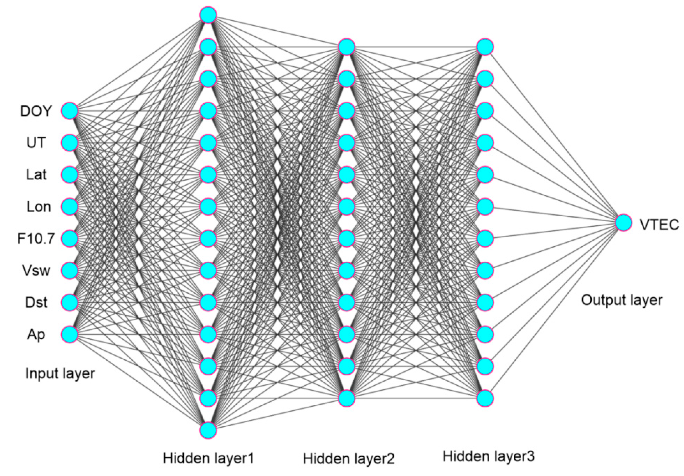
2.2. Artificial Neural Network-Based Australian TEC Model

The artificial neural network (ANN) technique is a promising tool in capturing the nonlinear relationships between multiple variables, and is formed by large numbers of simple processing elements known as neurons. This technique has been widely applied in ionospheric modeling, data classification, image recognition, etc. [26]. Backpropagation (BP) is one of the most successful algorithms in the ANN training process, which consists of two stages: feed-forward and back-forward. In a feed-forward process, the input datasets are studied by the ANN technique to generate predicted values, and the predicted errors are computed by the difference between target values and predicted values. In a back-forward process, the predicted errors are transferred from the output layer to the input layer, and then the input weights are adjusted. In this study, a simple BP neural network formed by an input layer, three hidden layers, and an output layer is utilized to develop an Australian TEC model. A dataset consists of day of year (DOY), universal time (UT), geographic latitude (Lat), geographic longitude (Lon), F10.7 cm solar flux (F10.7), solar wind speed (Vsw), Dst, and Ap is selected as input parameters. The vertical total electron content (VTEC) values in the output layer are estimated by the dual-frequency GNSS observation of the ARGN using pseudo-range observation smoothed with carrier phase [27]. Thousands of experiments are conducted to search the optimal combination of neural neurons in three hidden layers. The results indicate that the root-mean-square error (RMSE) is minimum when the numbers of neurons are 14, 12, 12 in three hidden layers, and the corresponding active functions in three hidden layers are tansig, tansig, and sigmod, respectively. The architecture of the ANN-based Australian TEC model is shown in Figure 2.

2.3. ANN-Aided SCHA Approach for Australian VTEC Modeling

Ionospheric TEC maps released by the International GNSS Services (IGS) have demonstrated that the spherical harmonics analysis is very suitable to develop ionospheric models on a global scale. However, the Legendre polynomial expansion in spherical harmonics is difficult to map the TEC over a regional area, the regional area is called as “cap”. The spherical cap harmonic analysis is available to develop a cap model well using the spherical cap coordinate system, and the spherical cap harmonic parameters can derive by solving a Laplace’s equation over a specific spherical cap. This method has been successfully applied to regional TEC models [7].
The zenith VTEC over a specific spherical cap can be expressed as:
V T E C ( θ , ξ ) = k = 0 k max m = 0 k [ P n k ( m ) m ( cos θ ) ( A k m · cos ( m · ξ ) + B k m · sin ( m · ξ ) ) ]
where (θ, ξ) is the coordinate of the ionospheric pierce point (IPP) in spherical cap coordinate, kmax is the maximum order, in this study kmax is set as 8. P n k ( m ) m ( cos θ ) is the normalized associated Legendre function where n and n k ( m ) are integral and real degrees, respectively. A k m and B k m are the normalized spherical cap harmonic coefficients. For more details about the spherical cap harmonic theory please refer to [27,28].
In this study, the Australian TEC maps can be estimated by the spherical cap harmonic method with the following steps:
(1)
The slant TEC along the path from a satellite to a receiver is estimated by the dual-frequency observations using pseudo-ranges smoothed with carrier phases, and the hardware differential code biases (DCB) of GNSS satellites and receivers are also corrected, please refer to [29]. The TEC in any epoch can be computed by the linear combination of pseudo-ranges and carrier phases as follows:
T E C p , k = f 1 2 f 2 2 40.28 ( f 1 2 f 2 2 ) ( P 2 P 1 ) + f 1 2 f 2 2 40.28 ( f 1 2 f 2 2 ) ( B p , r + B p s )
T E C ϕ , k = f 1 2 f 2 2 40.28 ( f 1 2 f 2 2 ) ( λ 2 ϕ 2 λ 1 ϕ 1 ) f 1 2 f 2 2 40.28 ( f 1 2 f 2 2 ) ( λ 2 N 2 λ 1 N 1 + B ϕ , r + B ϕ s )
where T E C p , k and T E C ϕ , k represent the TEC values derived from pseudo-range and carrier phase observations at epoch k, respectively. The subscripts r and s indicate the receiver and satellite, f1 and f2 are signal frequencies, Pi and ϕi are dual-frequency pseudo-range and carrier phase observations. λ1 and λ2 are the wavelengths of carrier phase l1 and l2, N1 and N2 are the ambiguities of carrier phase measurements (l1 and l2). B p , r and B p s are the receiver and satellite DCBs on the pseudo-range measurements, B ϕ , r and B ϕ s are the receiver and satellite DCBs on the carrier phase measurements. Usually, the receiver and satellites DCBs are regarded as stable in a few days [30], then
Δ T E C k = T E C p , k T E C ϕ , k = f 1 2 f 2 2 40.28 ( f 1 2 f 2 2 ) ( B p , r + B p s + λ 2 N 2 λ 1 N 1 + B ϕ , r + B ϕ s ) + f 1 2 f 2 2 40.28 ( f 1 2 f 2 2 ) ( P 2 P 1 + λ 2 ϕ 2 λ 1 ϕ 1 )
Generally, the ΔTECk is stable in a day, a more precise TEC observation can be computed by a recursive smoothing process.
Δ T E C = 1 N n = 1 N Δ T E C n = 1 N ( n = 1 N 1 Δ T E C n + Δ T E C N )
The smoothed ionospheric TEC calculates by:
Δ T E C k = f 1 2 f 2 2 40.28 ( f 1 2 f 2 2 ) ( λ 2 ϕ 2 λ 1 ϕ 1 ) + Δ T E C f 1 2 f 2 2 40.28 ( f 1 2 f 2 2 ) ( B p , r + B p s ) = f 1 2 f 2 2 40.28 ( f 1 2 f 2 2 ) ( λ 2 ϕ 2 λ 1 ϕ 1 ) + 1 N n = 1 N ( f 1 2 f 2 2 40.28 ( f 1 2 f 2 2 ) ( P 2 P 1 + λ 2 ϕ 2 λ 1 ϕ 1 ) ) f 1 2 f 2 2 40.28 ( f 1 2 f 2 2 ) ( B p , r + B p s ) = 1 N n = 1 N ( f 1 2 f 2 2 40.28 ( f 1 2 f 2 2 ) ( P 2 P 1 ) ) + 1 N n = 1 N 1 ( f 1 2 f 2 2 40.28 ( f 1 2 f 2 2 ) ( λ 2 ϕ 2 λ 1 ϕ 1 ) ) f 1 2 f 2 2 40.28 ( f 1 2 f 2 2 ) ( B p , r + B p s )
(2)
Convert the slant TEC (STEC) to the vertical TEC (VTEC) at a pierce point using the single-layer model function, the height of the single layer is set as 428.8 km.
(3)
Predict the TEC time series over the central points of the blank grid in Figure 1 using the ANN-based Australian TEC model, the blank grid means the regions where no experimental data are available.
(4)
Determine the pole point and the half-angle of the spherical cap to design the spherical cap coordinate system. According to the studying scope of the Australian map, the pole of the spherical cap is set as (−25°, 133°), the half-angle is determined as 20°, and the maximum order is chosen as 8.
(5)
Transform the coordinates of ionospheric pierce points and the central points of blank grids from the geographic coordinate system to the spherical cap coordinate system, Figure 3 illustrates the transformation relationship between the spherical cap coordinate system and the geographic coordinate system. If the geographic coordinates of the pole of the spherical cap are θP and λP, then the spherical cap coordinate (θC, λC) of any point Q (θ, λ) can be calculated using the following equations:
cos ( θ c )   =   cos ( θ P ) cos ( θ ) + sin ( θ P ) sin ( θ ) cos ( λ λ P ) tan ( π λ c )   =   sin ( θ ) sin ( λ λ P ) sin ( λ P ) cos ( θ ) cos ( θ P ) sin ( θ ) cos ( λ λ P )
(6)
Calculate the model coefficients ( A k m , B k m ) in Equation (1) using the least square method, and verify the performance of the estimated spherical cap model by comparing the model’s predicted TEC values with the TEC observations at the pierce points of GNSS stations.

3. Results

In this study, an artificial neural network-aided spherical cap harmonic analysis approach is proposed to estimate the Australian ionospheric TEC maps using long-term dual-frequency observations derived from the ARGN, the Australian ionospheric map is abbreviated as AIM. The Australian TEC maps are released with an interval of 15 min for geographic longitude and latitude in 0.5° × 0.5°.

3.1. Comparison with the AIMSCHA Model in 2013 and 2017

To evaluate the efficiency of the ANN technique in ionospheric modeling, the Australian TEC maps are also estimated only using the spherical cap harmonic analysis, namely AIMSCHA. The performances of the AIMs are validated in solar medium year (2013) and solar minimum year (2017) compared to the AIMSCHA maps, the TEC time series derived from the dual-frequency measurements of the ARGN stations are chosen as references. The comparative results are shown in Table 1.
As shown in Table 1, both the predicted RMSEs of the AIMSCHA and AIM maps in the solar minimum year are remarkably smaller than that in the solar medium year, and the RMSEs in summer and autumn are much smaller than that in spring and winter. Compared to the AIMSCHA model, the ANN technique could improve the predicted capability of the Australian TEC maps to a certain degree. The ratio is calculated as ( AIM AIM SCHA ) / AIM SCHA . For example, the predicted RMSEs of the AIM maps in spring, summer, autumn, and winter of 2013 are 3.41, 2.42, 2.54, and 3.65 TECU, which is about 9.31%, 9.70%, 9.93% and 4.95% smaller than the RMSEs of the AIMSCHA maps. This conclusion is also suitable in 2017, the predicted accuracies of the AIM maps improve about 8.86%, 10.28%, 8.20% and 6.61% than the AIMSCHA maps in spring, summer, autumn, and winter, respectively. The comparative results demonstrate that the ANN technique not only plays an important role in solving the “ill condition” when estimating the spherical cap harmonic function, but also improves the predicted accuracy of the AIM model with a degree of 8–10%, especially in high-level solar activities.

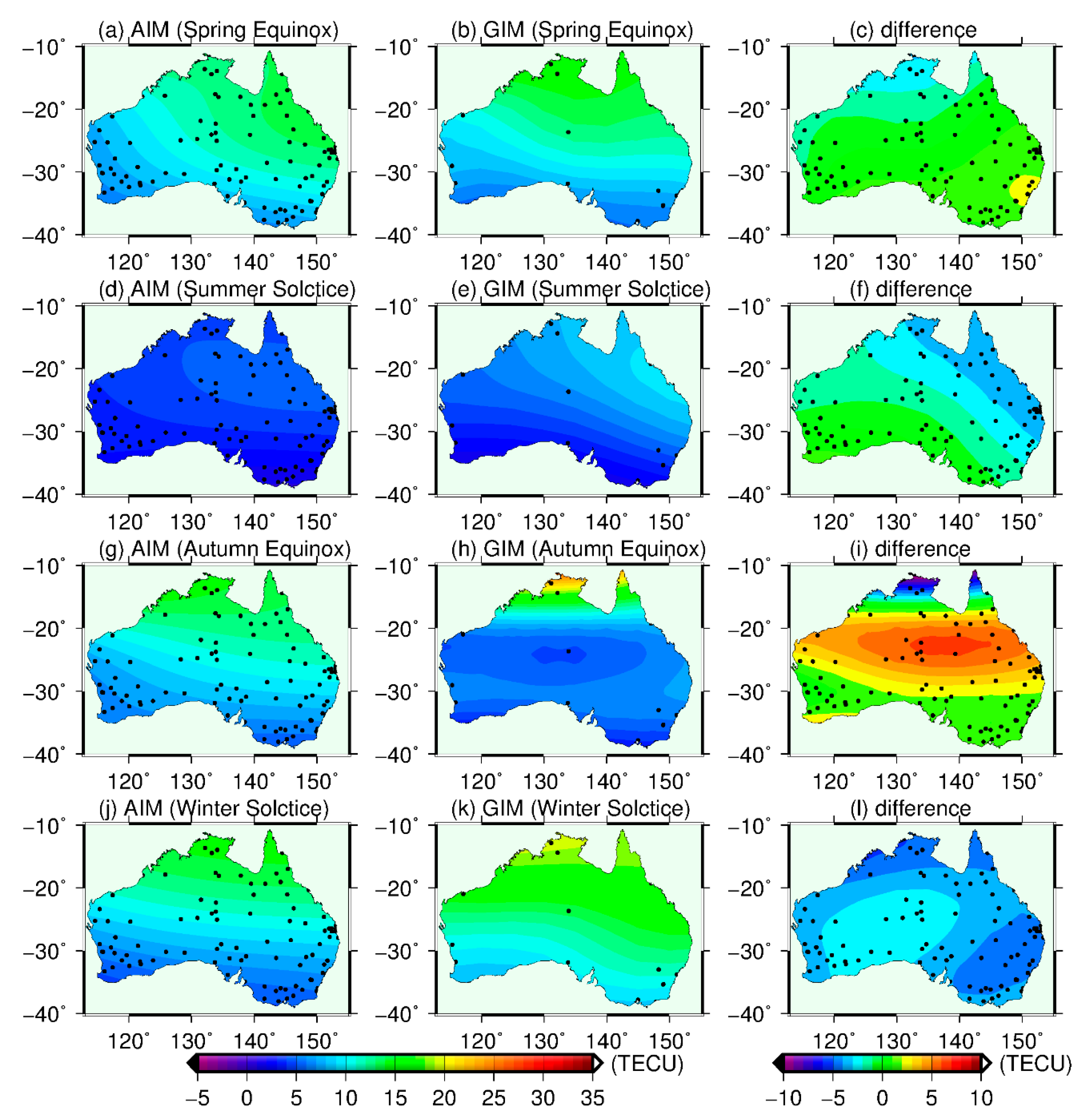
3.2. Seasonal and Hourly Features of the AIM Maps

To further validate the spatial characteristics of the AIM maps dependent on the level of solar radiation, the Australian TEC maps in different solar activity years 2009, 2012, 2014, and 2017 during the 23–24 solar cycles are estimated by the dual-frequency observations derived from the ARGN. The seasonal variations of the Australian TEC maps at the universal time (UT) 00:00 hour are shown in Figure 4. In this figure, the black points represent the ARGN’s stations which observations have passed the quality control stage. Figure 4a–d show that the GNSS stations of the ARGN network increasing rapidly from 2009, and most of these stations locate in the coastal areas, such as New South Wales, Victoria, Western Australia, etc. In Australia, the TEC value is inversely proportional to the geographic latitude, the TEC value in northern Australia is about two-times larger than that in the southern area. From 2009, with solar activity recovering to a normal level, the TEC value gradually increases and reaches to the maximum in 2014. Seasonal variations of Australian ionospheric maps show the TEC values in spring equinox and winter solstice are maximum, and in summer solstice the TEC value is minimum, which is caused by the revolution of the earth. Additionally, during the years 2009–2012 with the rising phase of solar radiation in solar cycle 24, the TEC values in spring equinox are lower than that in winter solstice; while the phenomenon is opposite in the declining phase (2014–2017) in the solar cycle 24.
Figure 5 shows the hourly variations of Australian TEC maps on the winter solstice of 2016. From Figure 5a at UT01:00, the TEC in Australia gradually enhances and reaches a maximum value of 30 TECU at UT05:00 (Figure 5e). After that, it begins to decrease and reaches a minimum value of 5 TECU at UT20:00. The high TECs appear in the period of UT04:00 (Figure 5d) to UT07:00 (Figure 5g), the corresponding local time (LT) is LT14:00 to LT17:00. The daytime TEC values over the northern area of Australia are 2–3 times larger than that in other regions, and the TEC variations over this region located at the south crest of the equatorial ionization anomaly are more violent. Figure 4 and Figure 5 demonstrate that the Australian TEC maps estimated by the SCHA method optimized by the ANN technique are consistent with the global ionospheric maps provided by the CODE [31], which indicates that the AIM model is successful to capture the spatial-temporal characteristics of Australian TEC variations well.

3.3. Mapping Performance of the AIM Model under Quiet and Disturbed Geomagnetic Conditions

3.3.1. Validation of the Mapping Performance under Quiet Geomagnetic Condition

The global ionosphere maps released by the IGS are estimated by the dual-frequency observations of more than 400 GNSS stations. Among them, only about 10 stations located in Australia are used. To evaluate the mapping accuracy of the AIM model under a quiet geomagnetic condition, the vertical TEC time series over four GNSS stations that have been used to develop the GIM and AIM models are selected as references. The names of four stations are MOBS (144.58° E, 37.49° S), CEDU (133.48° E, 31.52° S), DARW (131.08° E, 12.50° S), and SYDN (151.09° E, 33.46° S). They are distributed in Melbourne, Ceduna, Darwin, and Sydney, respectively. The predicted TEC values over the four stations are extracted from the products of the GIM and AIM models, namely GIM–TEC and AIM–TEC. The comparative results between true TEC, GIM–TEC, and AIM–TEC in the equinoxes and solstices of 2016 are shown in Figure 6.
Generally, the GIM–TEC and AIM–TEC values agree well with the true TEC time series, both the TEC maps success to reproduce the hourly dynamic features of ionospheric electron content over Australia. However, the RMSE and standard deviation (SD) of the AIM–TEC are smaller than the GIM–TEC, and the RMSEs and SDs of the AIM model are dependent on the season and geographic latitude remarkably. For the season, the accuracies of the AIM model in summer solstice and autumn equinox are highest, followed by winter solstice, while spring equinox is lowest. The phenomenon is caused by the level of seasonal solar radiation in 2016. From Figure 6e–h, it is found that the RMSEs of the TEC time series extracted from the AIMs over station MOBS, CEDU, DARW, and SYDN are 1.05, 1.04, 1.86, 1.26 TECU, respectively. The corresponding RMSEs of TEC time series derived from the GIMs over four stations are 1.18, 2.55, 3.03, and 1.67 TECU. For SDs, the indices of the AIMs over station MOBS, CEDU, DARW, and SYDN are 2.41, 2.39, 4.19, and 2.10 TECU, respectively, and the corresponding SDs for the GIMs are 3.10, 3.66, 5.32, and 3.10 TECU. The comparative results demonstrate that the Australian TEC maps estimated by the SCHA method with ANN-aided technique are superior to the GIMs remarkably, and the accuracies (RMSEs) of the AIM improve about 11%, 59%, 38.6% and 25% over the above stations compared to the GIMs. Besides, the mapping performance of the AIM model has a close relationship with the geographic latitude. For example, the RMSE of station DARW located in the northern area of Australia is maximum, the averaged predicted residual exceeds 3 TECU, and the maximum SD exceeds 10 TECU. Station DARW is located at the southern crest of equatorial ionization anomaly (EIA), where the equatorial ionosphere is very violent that controlled by the fountain effect [32], equatorial eastward electric field [33], thermospheric particle exchange [34], etc. The mapping performance of the AIM model over the station MOBS is best, which station is located in the southern area of Australia. The predicted RMSEs in four seasons (Figure 6a,e,i,m) are 1.58, 1.05, 1.12, and 1.48 TECU, respectively, and the improvements range from 5% to 40% compared to the GIMs. Furthermore, it is noted that sometimes the performance of the AIM model is worse than the GIM over the equatorial station. For example, in Figure 6c,k, the predicted RMSEs and SDs of the AIM for station DARW are larger than the GIM during spring and autumn. This limitation should be improved in future work.
Figure 1 shows the number of ARGN stations used for developing the AIM maps is much larger than the IGS stations located in Australia. To further validate the mapping performance of the AIM maps over the blank grid where no IGS observations are available, the TEC values estimated by the dual-frequency measurements of ARGN stations while do not belong to the IGS network are selected as the reference. The details of two stations are MRO1 (116.38° E, 26.41° S) and MCHL (148.08° E, 26.21° S). The comparative results between the AIM–TEC and GIM–TEC are shown in Figure 7. From the panels of the left column, the RMSEs of the AIM–TEC over station MRO1 at the spring equinox, summer solstice, autumn equinox, and winter solstice are 2.26, 1.68, 1.87, and 1.66 TECU, respectively, the mapping accuracies improve about 25.41%, 60.47%, 54.83%, and 44.30% compared to the GIMs. The SDs of the AIMs are also 16.61%, 38.39%, 27.25%, and 0.002% smaller than the GIMs at the corresponding equinoxes and solstices. For the station MCHL, the mapping performances of the AIM–TEC during four seasons improve by about 46.31%, 25.29%, 47.22%, and 37.08%. Figure 6 and Figure 7 demonstrate the AIM model has a more powerful capability in reproducing the high-accuracy TEC maps over the entire Australian continent.
The relationship between the mapping residual of the AIM model and the level of solar activity is investigated in Figure 8. In this study, the averaged RMSEs of the GNSS stations of the ARGN on the equinoxes and solstices during 2012–2017 are calculated, it is found that the RMSE of the ANN-TEC in June (Figure 8b) is minimum with an average mapping residual of 2 TECU. The RMSEs in March (Figure 8a) and December (Figure 8d) are maximum with an average residual of 3 to 3.5 TECU. Besides, the RMSE values within the period of UT04:00–UT12:00 (about LT14:00–LT22:00) are two-times larger than that in other hours, which is due to the high-level solar radiation and the ionospheric scintillations related with the low-latitudinal plasma bubbles after sunset.
Figure 8e shows the level of solar radiation enhances from 2012 and reaches a peak in 2014, and then the solar activity gradually declines. Meanwhile, the mapping residuals of the AIM model during 2013–2014 is significantly larger than that in the years 2016–2017. For example, in Figure 8d, the averaged RMSE of the AIM model during 2013–2014 is 3.5 TECU, which is 1.5 TECU larger than the mapping residuals at 2016–2017. The results demonstrate that the mapping performance of the AIM model has a close relationship with the level of solar radiation, and this model might achieve better performance under quiet solar conditions.
The above sections show that the AIM model developed by the SCHA method with the ANN-aided technique could successfully generate the high-accuracy Australian TEC map. To further investigate the spatial differences between the Australian TEC maps derived from the GIM and AIM model, the midday and midnight TEC maps on the equinoxes and solstices in 2016 are computed. From Figure 9, it is found that the spatial features of the AIM–TEC maps agree well with the GIMs, but the GIMs seem to hold a lead of several phases over the AIM’s maps. From the panels of the right column, the TEC values extracted from the AIMs are larger than the GIMs over Western Australia, but this phenomenon is opposite over eastern Australia. The positive difference is maximum on the summer solstice with a magnitude of 8 TECU at Western Australia, and the maximum negative difference covers the Queensland with a magnitude of −6 TECU during the winter solstice.
Figure 10 shows the spatial differences between the Australian TEC maps derived from the AIM and GIM at midnight. Generally, the spatial feature of the AIM map is consistent with the GIM map well, and the difference between the two kinds of maps at midnight is smaller than that at noon. The panels in the right column show that the differences in the spring equinox (Figure 10c) and summer solstice (Figure 10f) are minimum, and the magnitude ranges from −3 to 3 TECU. On the winter solstice (Figure 10l), the AIM–TEC maps are smaller than the GIMs over the entire Australian continent, and the remarkable negative differences cover the northern and southeast Australia with a magnitude of exceeds –4 TECU. Especially on the autumn equinox (Figure 10i), the TEC values of the AIM maps are remarkably larger than the GIMs over central-eastern Australia, the maximum amplitude reaches to 8 TECU. The remarkable TEC differences between the AIM and GIM maps are believed to be caused by different time resolutions. Since 2015, the CODE released a new version of global TEC map with a one-hour interval, while in this study the time resolution of the Australian TEC map based on the SCHA method is 15 min. The AIM map has an averaged 30-min phase delay compared to the GIM. The midday ionospheric variation affected by the strong solar radiation is very violent, therefore the midday spatial differences between the two models are more remarkable than that at midnight.

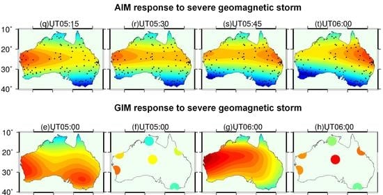
3.3.2. Validation of the Mapping Performance under the Severe Geomagnetic Condition

Section 3.3.1 demonstrates that the AIM model has a good mapping performance under quiet geomagnetic conditions. In this section, we will further investigate the mapping performance of the AIM model under a severe geomagnetic storm. The severe geomagnetic storm on 22 June 2015, is selected as a case study, and the response of the AIM maps to this geomagnetic storm is analyzed. The variation of the GIM map within the period of the violent storm is also investigated for comparison. This geomagnetic storm started from UT19:00, June 22, and reached the most violent at UT04:30, June 23 with a maximum of Dst value of −207nT. The geomagnetic condition on 21 June 2015, was quiet, hence the TEC values on the day are utilized as reference values. The TEC responses of the AIM and GIM to the geomagnetic event are shown in Figure 11 and Figure 12, respectively.
In Figure 11, the maps represent the Australian TEC responses of the AIM map to the severe geomagnetic storm, and the dots represent the TEC variations derived from the dual-frequency measurements of the IGS stations under disturbed geomagnetic conditions. The ratio of TEC variation is computed by ( TEC disturbed TEC quiet ) / TEC quiet . From Figure 11, it is found that the remarkable ionospheric TEC disturbances appeared from UT03:15 (Figure 11a), the AIM–TEC enhanced about 160% over the western Australia compared to the references, and the magnitude of the TEC enhancement over eastern Australia was about 40–80%. Then the intensity of ionospheric disturbances gradually grew more violent, until UT05:00 (Figure 11l) the ratio of TEC enhancement over the western Australia sharply reached 320%, and the AIM–TEC variations over the central-eastern Australian area also enhanced 240%. During the period of UT05:00 to 6:00, the violent TEC disturbances travelled from the western Australia to the Queensland state with a maximum enhancement of 260% to 300%. After that, the intensity of the ionospheric response to the geomagnetic storm began to decline. At UT08:00, the intense TEC perturbation appeared in the Queensland state with a positive ratio of 120%, and in other regions, the ratio of TEC enhancement was under 80%.
Generally, the TEC responses derived from the dual-frequency measurements of IGS stations (hereinafter referred to as IGS–TEC) were consistent with the AIM–TEC variations, but the magnitudes of IGS–TEC response are stronger than the AIM–TEC, especially during the main phase of the magnetic storm (about 05:00–06:00). For example, in Figure 11v,w, the magnitudes of the IGS–TEC enhancements over the western Australia and Queensland state ranged from 280% to 320%, while the amplitudes of the AIM–TEC disturbances were within 240% to 260%. Besides, the remarkable differences of the TEC responses between AIM and IGS were also observed in Victorian, the IGS–TEC responses were more violent than the AIM–TEC with a magnitude of exceeds 120%. Briefly, the ionospheric TEC perturbations extracted from the Australian TEC maps under severe geomagnetic storms agree well with the true TEC responses estimated by the dual-frequency observations of IGS stations, but the magnitude of the AIM–TEC response is relatively lower than the IGS–TEC disturbances during the main phase of the geomagnetic storm.
Same as the AIM–TEC responses in Figure 11, the TEC responses derived from the GIM maps under great magnetic storms are shown in Figure 12. It is found that the spatial TEC disturbances derived from the GIM maps were consistent with the AIM–TEC anomalies, but the GIM maps with an interval of 1 hour were failed to capture the precise dynamic features of Australian TEC response to this magnetic storm compared to the AIM maps. From Figure 11i–t, the violent ionospheric TEC disturbances during UT04:00–06:00 travelled from the western Australian to the Queensland state, but the GIM maps could not capture the electrodynamic features of traveling TEC disturbances. The GIM maps was not able to monitor the strength of TEC disturbances with high accuracy. For example, in Figure 12h, the TEC responses derived from the GNSS observations enhanced about 320% over the western Australian at UT06:00, while the magnitude of the GIM–TEC responses reached to 240%. The remarkable retrieving error was also observed at UT07:00. Therefore, the results indicate that the GIM maps are not available to detect the adequate electrodynamic evolution of traveling ionospheric disturbances under severe geomagnetic storms.

4. Discussion

In this paper, the ANN technique is used to generate the TEC values over the “no-stations” grids for improving the “ill-conditions” problem while establishing the Australian TEC model. Previous studies have demonstrated that the ANN technique is very effective in modeling the Australian TEC maps. For example, Bouya et al. [35] proposed an approach based on the combined use of the ANN and principal component analysis (PCA) to build an Australian regional TEC model at the Ionospheric Prediction Service (IPS), and the PCA–ANN Australian TEC model achieved a good result. The application of the spherical cap harmonic analysis in mapping the Australian TEC maps was also validated by [36]; the regional TEC model well captures the basic spatial-temporal ionospheric features over Australia, and the obtained results confirm the usefulness of the SCHA method for near real-time mapping TEC values over the Australian continent. In this study, we assimilate the advantages of the previous studies and establish an AIM model using the SCHA method with the ANN-aided technique. The new AIM model shows a powerful capability in capturing the spatial-temporal characteristics of the Australian TEC maps. This model not only maps the Australian TEC with an RMSE of 2–3 TECU but also successes to reproduce the seasonally and hourly of the Australian ionospheric map.
Compared to the previous studies, the mapping residual of the AIM model is well. For example, Liu et al. [9] utilized the observations of 44 IGS stations to map the Arctic TEC maps by the SCHA method, the short-term prediction errors were ±2.2 TECU, ±3.8 TECU, and ±4.8 TECU for a latency of 1, 2, and 3 days, respectively. Ghoddousi-Fard et al. [8] processed the GPS data of about 75 stations to produce the daily and near-real-time VTEC maps over Canada and adjacent regions, the mean standard deviation of differences between regional SCHA and ionosphere map exchange (IONEX) maps agree well with the 1–2 TECU root mean square differences IGS reports. Okoh et al. [21] used the TEC measurements obtained from 269 ground-based GPS stations as well as from the COSMIC profiles for various parts of the Africa to develop an African TEC regional model (known as AfriTEC model), this model could success to map the equatorial anomaly crests over the African region. The averaged simulated residual of the AfriTEC model is 3.73 TECU that is higher than the AIM model in this study. The results may be associated with the insufficient TEC observations over the North Africa. The comparative results demonstrate that the SCHA method with the ANN-aided technique is helpful to enhance the regional TEC predict ability, especially for a continent that the GNSS stations are not located evenly.
However, it may be recalled here that the present version of the AIM model fails to map the TEC over the northern region of Australian well. In Figure 6c,k, the predicted residuals of the AIM model are larger than the GIM during equinoxes over the DARW station located in northern Australia. Northern Australia is located at the southern crest of the equatorial ionization anomaly (EIA), where the ionospheric physical mechanism is so complex that the ionospheric electrodynamic convention is controlled by the geomagnetic field, penetrating eastward electric field, neutral winds, etc. [31,37,38,39]. The violent ionospheric variations over the EIA region has a serious effect on the human activities in this area, especially for the single-frequency receivers. The problem of low mapping performance of the AIM model over northern Australia will be improved in our future studies.

5. Conclusions

In this study, the long-term dual-frequency observations obtained from the ARGN network are used to develop the Australian TEC model by the spherical cap harmonic analysis method optimized by the artificial neural network technique, and the performances of the Australian TEC model are evaluated over large spatial-temporal scales and under quiet-disturbed space weather conditions compared to the GIMs. The promising results indicate the GNSS stations of the ARGN network are sufficient to develop an Australian ionospheric model for mapping TEC using the SCHA method, and the ANN technique could improve the accuracy of TEC mapping approximately 8–10%, compared to the Australian TEC model built by only the SCHA method. The mapping accuracy of the AIM model is inversely proportional to the level of solar activity. Under quiet space weather conditions, the residuals of the AIM model in the spring equinox, summer solstice, autumn equinox, and winter solstice of the minimum solar activity year (2009) are 2.16, 1.57, 1.68, and 1.98 TECU, respectively. The residuals of the AIM model are also dependent on seasons and geographic locations remarkably. The residuals in the summer solstice and autumn equinox are smaller than that the one in spring equinox and winter solstice, and the residuals over the middle geographic latitudes are smaller than the low latitudes. Compared to the conventional global ionosphere map model, the mapping accuracy of the AIM model is 1–2 TECU higher than the GIM model with an improved amplitude of 10–50%. The spatial differences between the TEC maps show that the GIMs has a phase delay compared to the AIMs because of its low time resolution. In the western Australian the TEC values derived from the AIM maps are 5–8 TECU higher than the GIMs; while in eastern Australia the AIMs are lower than the GIMs with a maximum amplitude of −5 TECU. Furthermore, the spatial-temporal variations of the AIM maps agree well with the TEC time series estimated by the pseudo-range observation smoothed with carrier phase, and the AIM maps have a strong capability in capturing the adequate electrodynamic evolutions of the traveling ionospheric disturbances under severe geomagnetic storms.
Since 25 June 2019, the FormoSat-7/COSMIC-2 constellation consists of six remote sensing microsatellites that were launched to collect atmosphere-ionosphere-thermosphere profiles for weather prediction, climate change, and gravity research. This project could provide more than 4000 high-quality electron density profiles per-day within the ±40°geographic latitude, which will be helpful to profile the accurate dynamic structure of electron density over Australia. Therefore, in a further study, a complete Australian three-dimensional electron density model will be developed by the ionospheric tomography technique using multiple observations derived from the ground-based GNSS stations and the space-borne COSMIC-2 mission, which will further strongly support human activities that rely on the GNSS technique in this area.

Author Contributions

Conceptualization, W.L. and K.Z.; methodology, W.L. and D.Z.; software, W.L.; validation, W.L., D.Z. and Y.S.; formal analysis, W.L. and D.Z.; writing—original draft preparation, W.L. and D.Z.; writing—review and editing, W.L. and K.Z.; funding acquisition, K.Z. All authors have read and agreed to the published version of the manuscript.

Funding

This research was funded by the National Natural Science Foundations of China, grant number 41730109, the Natural Science Foundation of Jiangsu Province, China, grant number BK20200646, BK20200664, the Project funded by China Postdoctoral Science Foundation, grant number 2020M671645, the Fundamental Research Funds for the Central Universities, grant number 2020QN31, 2020QN30, the Open Fund of Key Laboratory for Synergistic Prevention of Water and Soil Environmental Pollution, grant number KLSPWSEP-A06, A Project Funded by the Priority Academic Program Development of Jiangsu Higher Education Institutions (Surveying and Mapping), and the Jiangsu Dual Creative Talents and Jiangsu Dual Creative Teams Programme Projects awarded in 2017.

Acknowledgments

The authors are very grateful to the Geoscience Australia for providing the observations of the Australian Regional GPS Network, the International GNSS Service for providing GNSS station measurements, the UNAVCO for providing the TEQC software.

Conflicts of Interest

The authors declare no conflict of interest.

References

  1. Hernández-Pajares, M.; Juan, J.M.; Sanz, J.; Aragón-Àngel, À.; García-Rigo, A.; Salazar, D.; Escudero, M. The ionosphere: Effects, GPS modeling and the benefits for space geodetic techniques. J. Geod. 2011, 85, 887–907. [Google Scholar] [CrossRef]
  2. Wang, N.; Yuan, Y.; Li, Z.; Li, Y.; Huo, X.; Li, M. An examination of the Galileo NeQuick model: Comparison with GPS and JASON TEC. GPS Solut. 2017, 21, 605–615. [Google Scholar] [CrossRef]
  3. Hoque, M.M.; Jakowski, N.; Berdermann, J. Ionospheric correction using NTCM driven by GPS Klobuchar coefficients for GNSS applications. GPS Solut. 2017, 21, 1563–1572. [Google Scholar] [CrossRef]
  4. Ho, C.; Wilson, B.; Mannucci, A.; Lindqwister, U.; Yuan, D. A comparative study of ionospheric total electron content measurements using global ionospheric maps of GPS, TOPEX radar, and the Bent model. Radio Sci. 1997, 32, 1499–1512. [Google Scholar] [CrossRef]
  5. Bilitza, D.; Altadill, D.; Truhlik, V.; Shubin, V.; Galkin, I.; Reinisch, B.; Huang, X. International Reference Ionosphere 2016: From ionospheric climate to real-time weather predictions. Space Weather 2017, 15, 418–429. [Google Scholar] [CrossRef]
  6. Olga Maltseva, G.G. Comparison of TEC prediction methods in mid-latitudes with GIM maps. Geod. Geodyn. 2020, 11, 174–181. [Google Scholar] [CrossRef]
  7. Liu, J.; Chen, R.; Wang, Z.; Zhang, H. Spherical cap harmonic model for mapping and predicting regional TEC. GPS Solut. 2011, 15, 109–119. [Google Scholar] [CrossRef]
  8. Ghoddousi-Fard, R.; Héroux, P.; Danskin, D.; Boteler, D. Developing a GPS TEC mapping service over Canada. Space Weather 2011, 9, 1–10. [Google Scholar] [CrossRef]
  9. Jiachun, A.; Zemin, W.; Xinguo, N. GPS-based regional ionospheric models and their suitability in Antarctica. Adv. Polar Sci. 2015, 25, 32–37. [Google Scholar]
  10. Liu, J.; Chen, R.; An, J.; Wang, Z.; Hyyppa, J. Spherical cap harmonic analysis of the Arctic ionospheric TEC for one solar cycle. J. Geophys. Res. Space Phys. 2014, 119, 601–619. [Google Scholar] [CrossRef]
  11. Razin, M.-R.G.; Voosoghi, B. Ionosphere tomography using wavelet neural network and particle swarm optimization training algorithm in Iranian case study. Gps Solut. 2017, 21, 1301–1314. [Google Scholar] [CrossRef]
  12. Li, Z.; Yuan, Y.; Wang, N.; Hernandez-Pajares, M.; Huo, X. SHPTS: Towards a new method for generating precise global ionospheric TEC map based on spherical harmonic and generalized trigonometric series functions. J. Geod. 2015, 89, 331–345. [Google Scholar] [CrossRef]
  13. Sivavaraprasad, G.; Deepika, V.S.; SreenivasaRao, D.; Kumar, M.R.; Sridhar, M. Performance evaluation of neural network TEC forecasting models over equatorial low-latitude Indian GNSS station. Geod. Geodyn. 2020, 11, 192–201. [Google Scholar] [CrossRef]
  14. Astafyeva, E.; Zakharenkova, I.; Huba, J.; Doornbos, E.; Van den IJssel, J. Global ionospheric and thermospheric effects of the June 2015 geomagnetic disturbances: Multi-instrumental observations and modeling. J. Geophys. Res. Space Phys. 2017, 122, 11716–11742. [Google Scholar] [CrossRef] [Green Version]
  15. Moses, M.; Dodo, J.D.; Ojigi, L.M.; Lawal, K. Regional TEC modelling over Africa using deep structured supervised neural network. Geod. Geodyn. 2020, 11, 367–375. [Google Scholar] [CrossRef]
  16. Ramazan Atıcı, S.S. Global investigation of the ionospheric irregularities during the severe geomagnetic storm on September 7–8, 2017. Geod. Geodyn. 2020, 11, 211–221. [Google Scholar] [CrossRef]
  17. Li, S.; Zhou, H.; Xu, J.; Wang, Z.; Li, L.; Zheng, Y. Modeling and analysis of ionosphere TEC over China and adjacent areas based on EOF method. Adv. Space Res. 2019, 64, 400–414. [Google Scholar] [CrossRef]
  18. Chang, X.; Zou, B.; Guo, J.; Zhu, G.; Li, W.; Li, W. One sliding PCA method to detect ionospheric anomalies before strong Earthquakes: Cases study of Qinghai, Honshu, Hotan and Nepal earthquakes. Adv. Space Res. 2017, 59, 2058–2070. [Google Scholar] [CrossRef]
  19. Zhang, Z.; Pan, S.; Gao, C.; Zhao, T.; Gao, W. Support Vector Machine for Regional Ionospheric Delay Modeling. Sensors 2019, 19, 2947. [Google Scholar] [CrossRef] [Green Version]
  20. Tulasi Ram, S.; Sai Gowtam, V.; Mitra, A.; Reinisch, B. The improved two-dimensional artificial neural network-based ionospheric model (ANNIM). J. Geophys. Res. Space Phys. 2018, 123, 5807–5820. [Google Scholar] [CrossRef]
  21. Okoh, D.; Seemala, G.; Rabiu, B.; Habarulema, J.B.; Jin, S.; Shiokawa, K.; Otsuka, Y.; Aggarwal, M.; Uwamahoro, J.; Mungufeni, P. A neural network-based ionospheric model over Africa from Constellation Observing System for Meteorology, Ionosphere, and Climate and Ground Global Positioning System observations. J. Geophys. Res. Space Phys. 2019, 124, 10512–10532. [Google Scholar] [CrossRef]
  22. Huang, Z.; Yuan, H. Ionospheric single-station TEC short-term forecast using RBF neural network. Radio Sci. 2014, 49, 283–292. [Google Scholar] [CrossRef]
  23. Mohammadi, B.; Linh, N.T.T.; Pham, Q.B.; Ahmed, A.N.; Vojteková, J.; Guan, Y.; Abba, S.; El-Shafie, A. Adaptive neuro-fuzzy inference system coupled with shuffled frog leaping algorithm for predicting river streamflow time series. Hydrol. Sci. J. 2020, 65, 1738–1751. [Google Scholar] [CrossRef]
  24. Hu, A.; Carter, B.; Currie, J.; Norman, R.; Wu, S.; Wang, X.; Zhang, K. Modeling of topside ionospheric vertical scale height based on ionospheric radio occultation measurements. J. Geophys. Res. Space Phys. 2019, 124, 4926–4942. [Google Scholar] [CrossRef]
  25. Takahashi, H.; Wrasse, C.; Denardini, C.; Pádua, M.; de Paula, E.; Costa, S.; Otsuka, Y.; Shiokawa, K.; Monico, J.G.; Ivo, A. Ionospheric TEC weather map over South America. Space Weather 2016, 14, 937–949. [Google Scholar] [CrossRef] [Green Version]
  26. Li, W.; Zhao, D.; He, C.; Hu, A.; Zhang, K. Advanced Machine Learning Optimized by The Genetic Algorithm in Ionospheric Models Using Long-Term Multi-Instrument Observations. Remote Sens. 2020, 12, 866. [Google Scholar] [CrossRef] [Green Version]
  27. Haines, G. Spherical cap harmonic analysis. J. Geophys. Res. Solid Earth 1985, 90, 2583–2591. [Google Scholar] [CrossRef]
  28. Haines, G. Computer programs for spherical cap harmonic analysis of potential and general fields. Comput. Geosci. 1988, 14, 413–447. [Google Scholar] [CrossRef]
  29. Sardon, E.; Rius, A.; Zarraoa, N. Estimation of the transmitter and receiver differential biases and the ionospheric total electron content from Global Positioning System observations. Radio Sci. 1994, 29, 577–586. [Google Scholar] [CrossRef]
  30. Hernández-Pajares, M.; Juan, J.; Sanz, J.; Orus, R.; Garcia-Rigo, A.; Feltens, J.; Komjathy, A.; Schaer, S.; Krankowski, A. The IGS VTEC maps: A reliable source of ionospheric information since 1998. J. Geod. 2009, 83, 263–275. [Google Scholar]
  31. Guo, J.; Li, W.; Liu, X.; Kong, Q.; Zhao, C.; Guo, B. Temporal-spatial variation of global GPS-derived total electron content, 1999–2013. PLoS ONE 2015, 10, e0133378. [Google Scholar] [CrossRef] [PubMed]
  32. Lin, C.-H.; Wang, W.; Hagan, M.E.; Hsiao, C.; Immel, T.; Hsu, M.; Liu, J.; Paxton, L.; Fang, T.-W.; Liu, C. Plausible effect of atmospheric tides on the equatorial ionosphere observed by the FORMOSAT-3/COSMIC: Three-dimensional electron density structures. Geophys. Res. Lett. 2007, 34, L11112. [Google Scholar] [CrossRef] [Green Version]
  33. Li, W.; Yue, J.; Guo, J.; Yang, Y.; Zou, B.; Shen, Y.; Zhang, K. Statistical seismo-ionospheric precursors of M7. 0+ earthquakes in Circum-Pacific seismic belt by GPS TEC measurements. Adv. Space Res. 2018, 61, 1206–1219. [Google Scholar] [CrossRef]
  34. Li, W.; Yue, J.; Yang, Y.; He, C.; Hu, A.; Zhang, K. Ionospheric and thermospheric responses to the recent strong solar flares on 6 september 2017. J. Geophys. Res. Space Phys. 2018, 123, 8865–8883. [Google Scholar] [CrossRef] [Green Version]
  35. Bouya, Z.; Terkildsen, M.; Francis, M. Total electron content forecast model over Australia. In Proceedings of the 40th COSPAR Scientific Assembly, Moscow, Russia, 2–10 August 2014. [Google Scholar]
  36. Bouya Zahra, T.M.; Dave, N. Regional GPS-based ionospheric TEC model over Australia using Spherical Cap Harmonic Analysis. In Proceedings of the 38th COSPAR Scientific Assembly, Bremen, Germany, 18–15 July 2010; Volume 38, p. 4. [Google Scholar]
  37. Raghavarao, R.; Nageswararao, M.; Sastri, J.H.; Vyas, G.; Sriramarao, M. Role of equatorial ionization anomaly in the initiation of equatorial spread F. J. Geophys. Res. Space Phys. 1988, 93, 5959–5964. [Google Scholar] [CrossRef]
  38. Sai Gowtam, V.; Tulasi Ram, S. Ionospheric annual anomaly—New insights to the physical mechanisms. J. Geophys. Res. Space Phys. 2017, 122, 8816–8830. [Google Scholar] [CrossRef]
  39. Wang Li, J.Y.; Suqin, W.; Yang, Y.; Zhen, L.; Jingxue, B.; Kefei, Z. Ionospheric responses to typhoons in Australia during 2005–2014 using GNSS and FORMOSAT-3/COSMIC measurements. GPS Solut. 2018, 22, 61. [Google Scholar]
Figure 1. Geographic distribution of the stations of the Australian Regional GPS Network, the background map is the digital elevation map.
Remotesensing 12 03851 g001
Figure 2. Architecture of the ANN-based Australia total electron content (TEC) model.
Remotesensing 12 03851 g002
Figure 3. Transformation relationship between geographic coordinate system and spherical cap coordinate system.
Remotesensing 12 03851 g003
Figure 4. Spatial variations of the Australian TEC maps in the equinoxes and solstices, the time of each subfigure is universal time 00:00. (ad) show the Australian TEC maps in spring equinox during 2009–2017, (eh) in summer solstice, (il) in autumn equinox, (mp) in winter solstice.
Remotesensing 12 03851 g004
Figure 5. Hourly Australian TEC maps predicted by the AIM model on the winter solstice in 2016, (ax) show the temporal variations of Australian TEC maps from UT01:00 to UT24:00 with an interval of one hour.
Remotesensing 12 03851 g005
Figure 6. Comparative results of the performances of the GIM and AIM over Stations MOBS, CEDU, DARW, and SYDN in 2016, the red and green lines indicate the GIM and AIM time series, (ad) show the comparative results over Stations MOBS, CEDU, DARW, and SYDN in spring equinox, (eh) in summer solstice, (il) in autumn equinox, (mp) in winter solstice.
Remotesensing 12 03851 g006
Figure 7. Similar to Figure 6, but for stations MRO1 and MCHL, (a,c,e,g) show the comparative results over station MRO1 in spring equinox, summer solstice, autumn equinox and winter solstice, (b,d,f,h) over station MCHL.
Remotesensing 12 03851 g007
Figure 8. Mapping performances of the AIM maps during 2012–2017, the RMSEs of AIM–TEC maps are computed in (a) spring equinox, (b) summer solstice, (c) autumn equinox and (d) winter solstice, respectively, (e) shows the F10.7 solar flux time series during 2012–2018.
Remotesensing 12 03851 g008
Figure 9. Spatial differences between the Australian TEC maps mapped by the AIM and GIM at local time 12:00, 1 January 2016, the black points represent the GNSS stations, (a,d,g,j) show the TEC maps derived from the AIM model in spring equinox, summer solstice, autumn equinox and winter solstice, (b,e,h,k) show the TEC maps derived from the GIM model, (c,f,i,l) show the differences between the TEC maps derived from the AIM and GIM.
Remotesensing 12 03851 g009
Figure 10. Similar to Figure 9, but at midnight, 1 January 2016, (a,d,g,j) show the TEC maps derived from the AIM model in spring equinox, summer solstice, autumn equinox and winter solstice, (b,e,h,k) show the TEC maps derived from the GIM model, (c,f,i,l) show the differences between the TEC maps derived from the AIM and GIM.
Remotesensing 12 03851 g010
Figure 11. TEC responses of the AIM map during the main phase of the severe geomagnetic storm on 23 June 2015, the time interval is 15 min, the dots indicate the TEC perturbations of the referenced IGS stations, (an1) show the magnitude of Australian TEC enhancements derived from the AIM maps during UT03:15–UT08:00 with an interval of 15 minutes.
Remotesensing 12 03851 g011
Figure 12. TEC responses of the GIM map during the main phase of the severe geomagnetic storm on 23 June 2015, the time interval is 15 min, (al) show the magnitude of Australian TEC enhancements derived from the GIM maps during UT03:00–UT08:00 with an interval of one hour.
Remotesensing 12 03851 g012
Table 1. Comparative results of the predicted root-mean-square errors (RMSEs) of the AIMSCHA and AIM maps in 2013 and 2017 (unit: TECU).
Year2013 (Medium)2017 (Minimum)
SeasonSpringSummerAutumnWinterSpringSummerAutumnWinter
AIMSCHA3.762.682.823.842.371.751.832.11
AIM3.412.422.543.652.161.571.681.98
Ratio9.31%9.70%9.93%4.95%8.86%10.28%8.20%6.16%
Publisher’s Note: MDPI stays neutral with regard to jurisdictional claims in published maps and institutional affiliations.

