Perspectives on the Structural Health Monitoring of Bridges by Synthetic Aperture Radar


 ,
,  ,
,  and
and 
Abstract
1. Introduction
2. Methodology
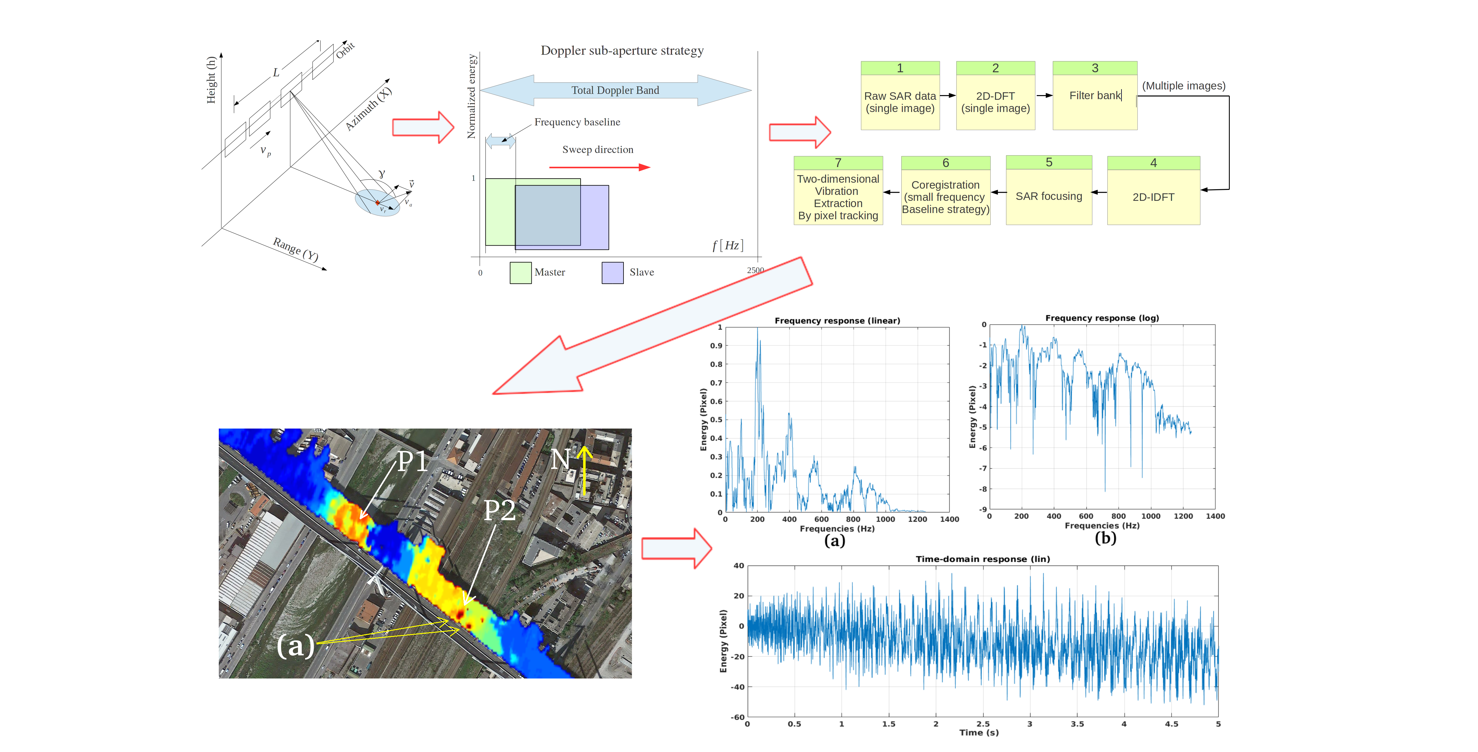
- r is the zero-Doppler distance (constant);
- R is the slant-range;
- is the reference range at ;
- is the physical antenna aperture length;
- V is the platform velocity;
- d is the distance between two range acquisitions;
- is the total synthetic aperture length;
- t is the acquisition time variable;
- T is the observation duration;
- and are the start and stop time acquisition respectively;
- is the azimuth electromagnetic footprint width;
- is the incidence angle of the electromagnetic radiation pattern;
- V is the platform velocity.
2.1. Doppler Sub-Apertures Model
- anomalous azimuth displacement in the presents of target constant range velocity;
- azimuth smearing in the presence of target azimuth velocity or target range accelerations;
- range-walking phenomenon, visible as range defocusing, in the presence of target range speed, backscattered energy is detected over one or more range resolution cells.
- (due to range velocity);
- (due to range acceleration);
- (due to azimuth velocity).
2.2. Vibrational Model of Infrastructures
- is the external force vector applied to the system over the time t;
- , and are the nodal displacement, the velocity, and the acceleration vectors, respectively;
- , and are the global mass, damping and stiffness matrices of the dynamic system, respectively.
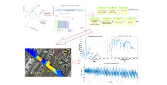
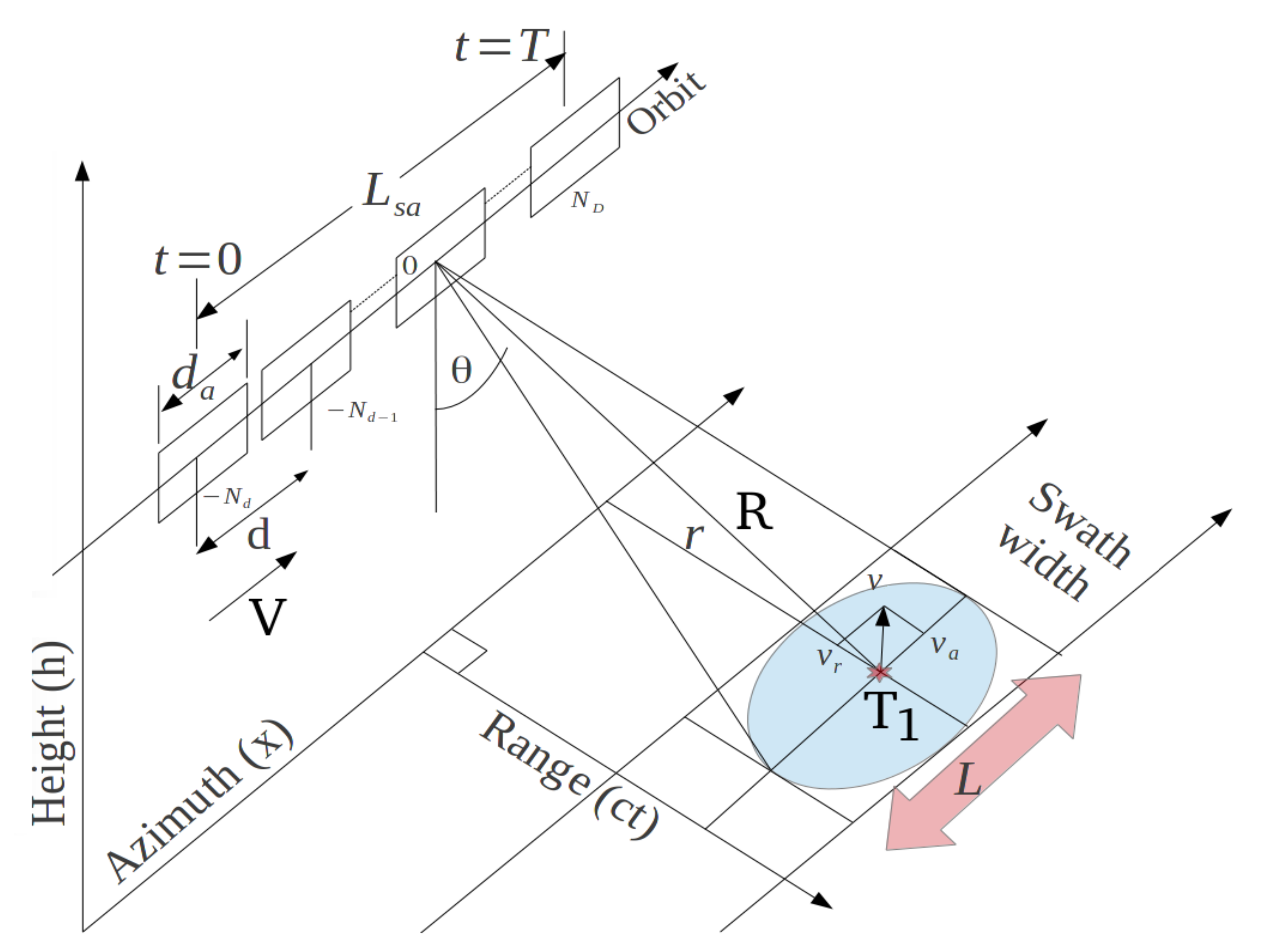
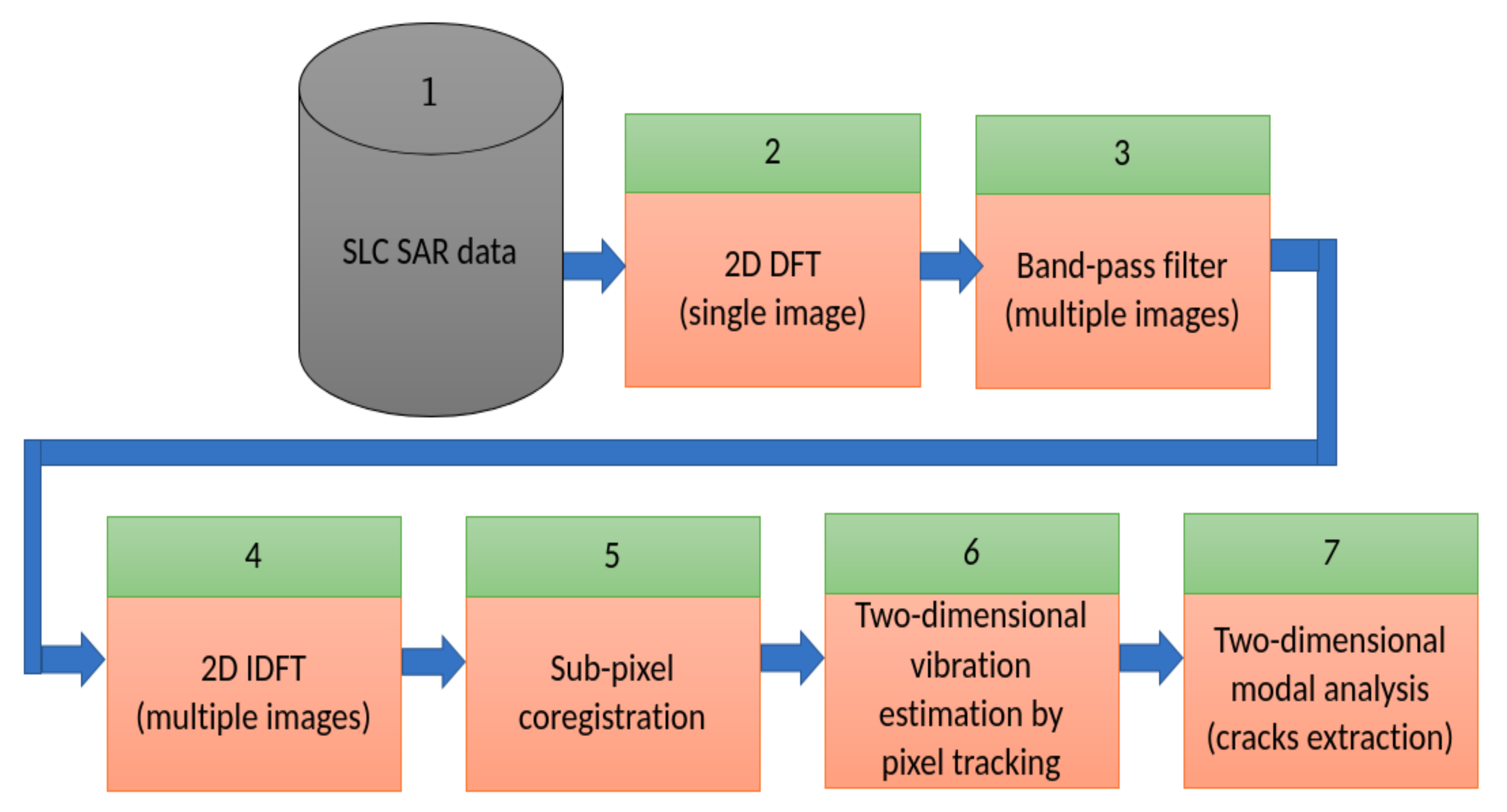
2.3. Processing Framework
- Selection of a single SLC-SAR image observing bridges.
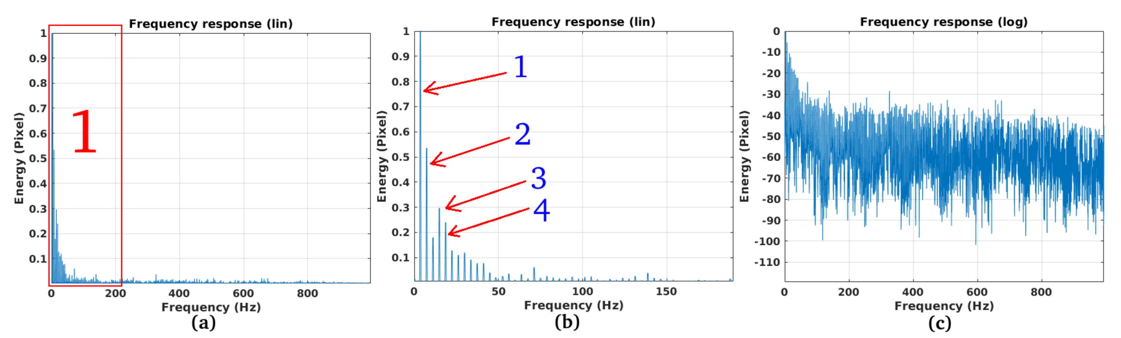
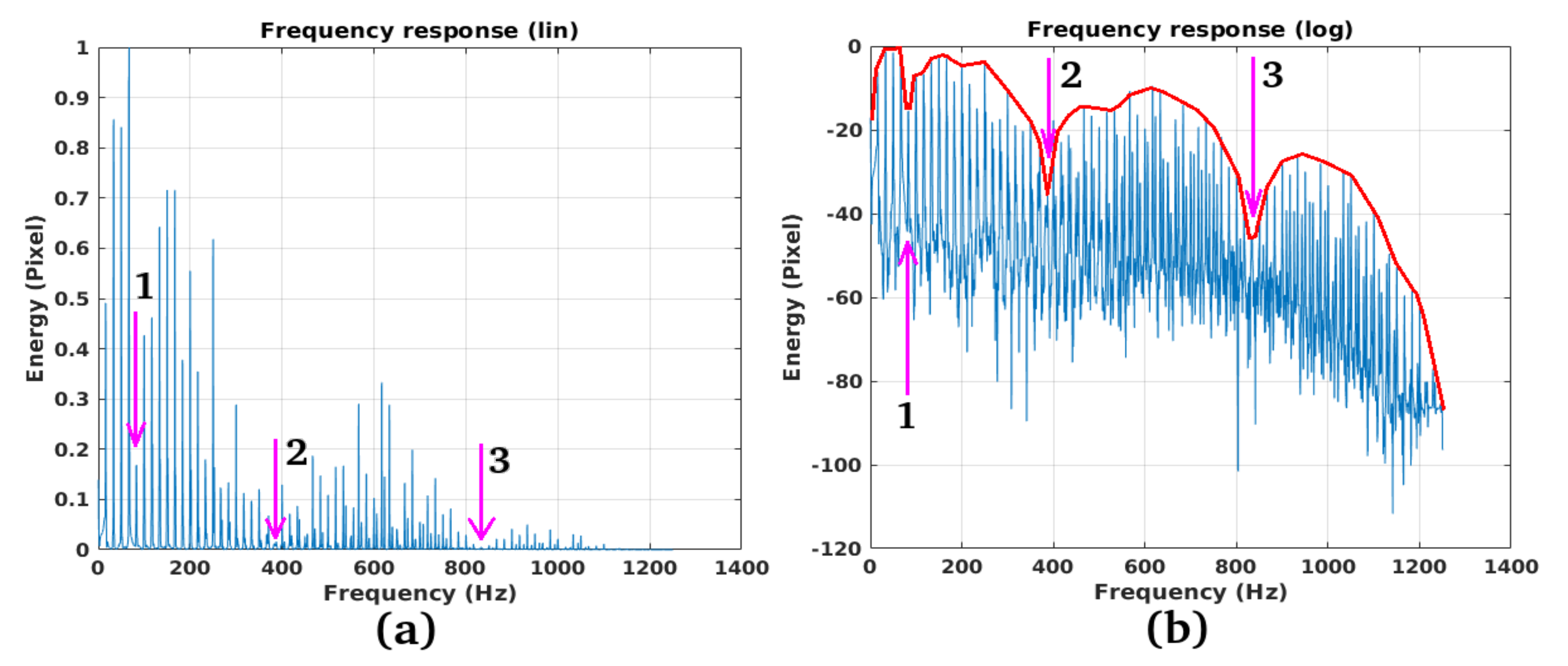
- Computation of the bi-dimensional spectrum via 2D-DFT.
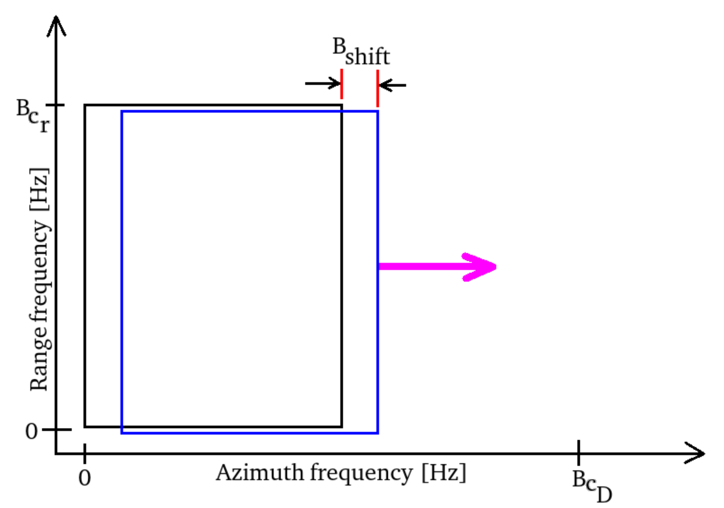
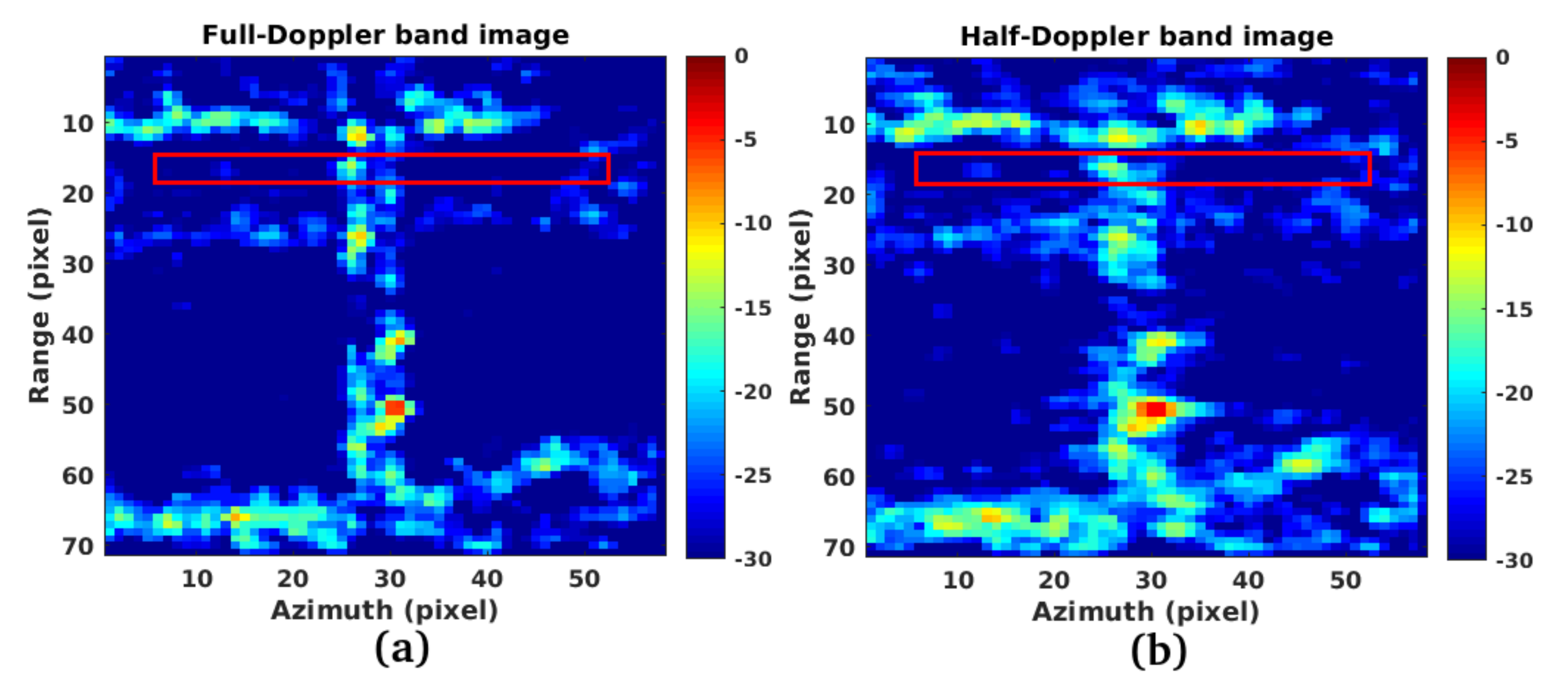
- Band-pass filtering according to the small-frequency baseline strategy of Figure 3. The output of the third block consists in multiple images centered at the consecutive different Doppler frequencies.
- Computation of the inverse 2D-DFT for retrieving the SLC SAR image with lower azimuth spatial resolution.
- Sub-pixel coregistration;
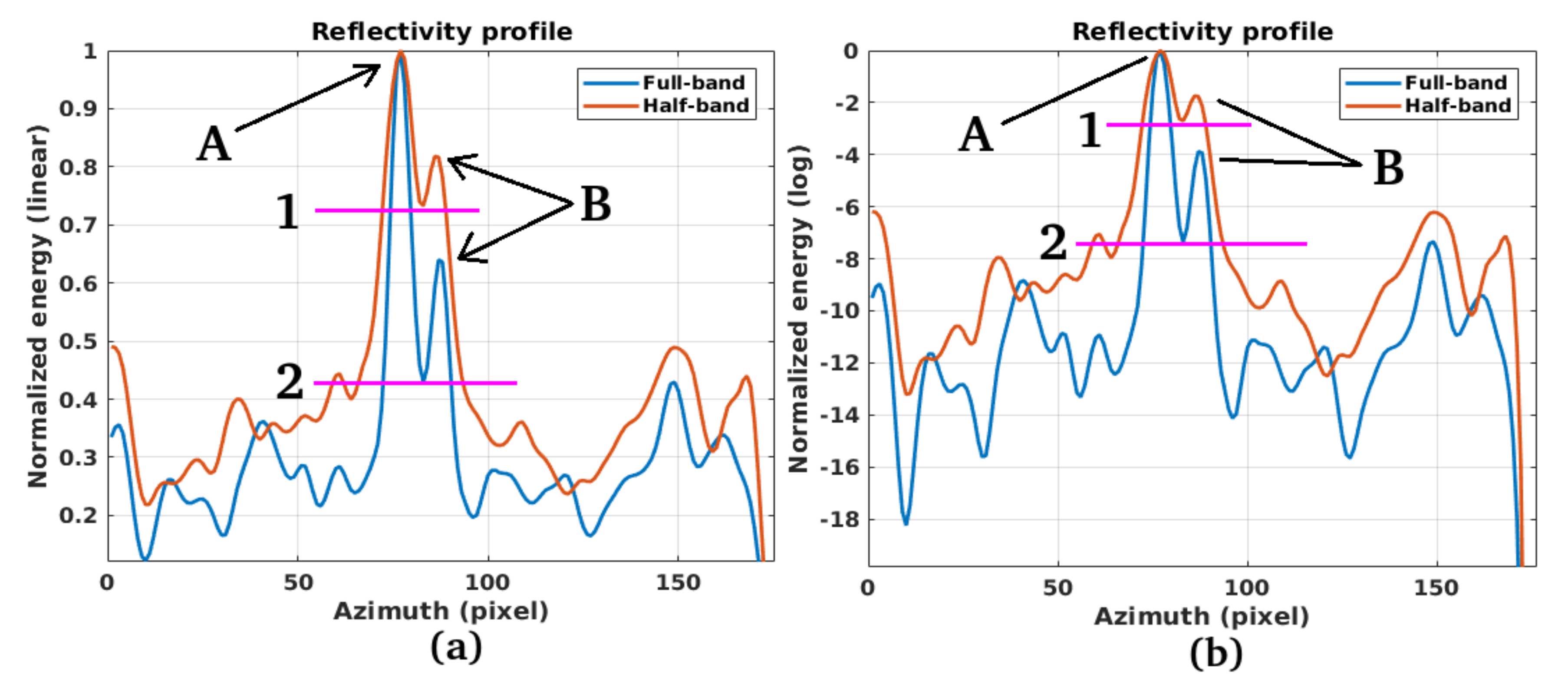
- Two dimensional vibration estimation by pixel tracking;
- Two-dimensional modal analysis for infrastructure crack extraction.
3. Analyses of Structural Integrity of Bridges from SAR
- (1)
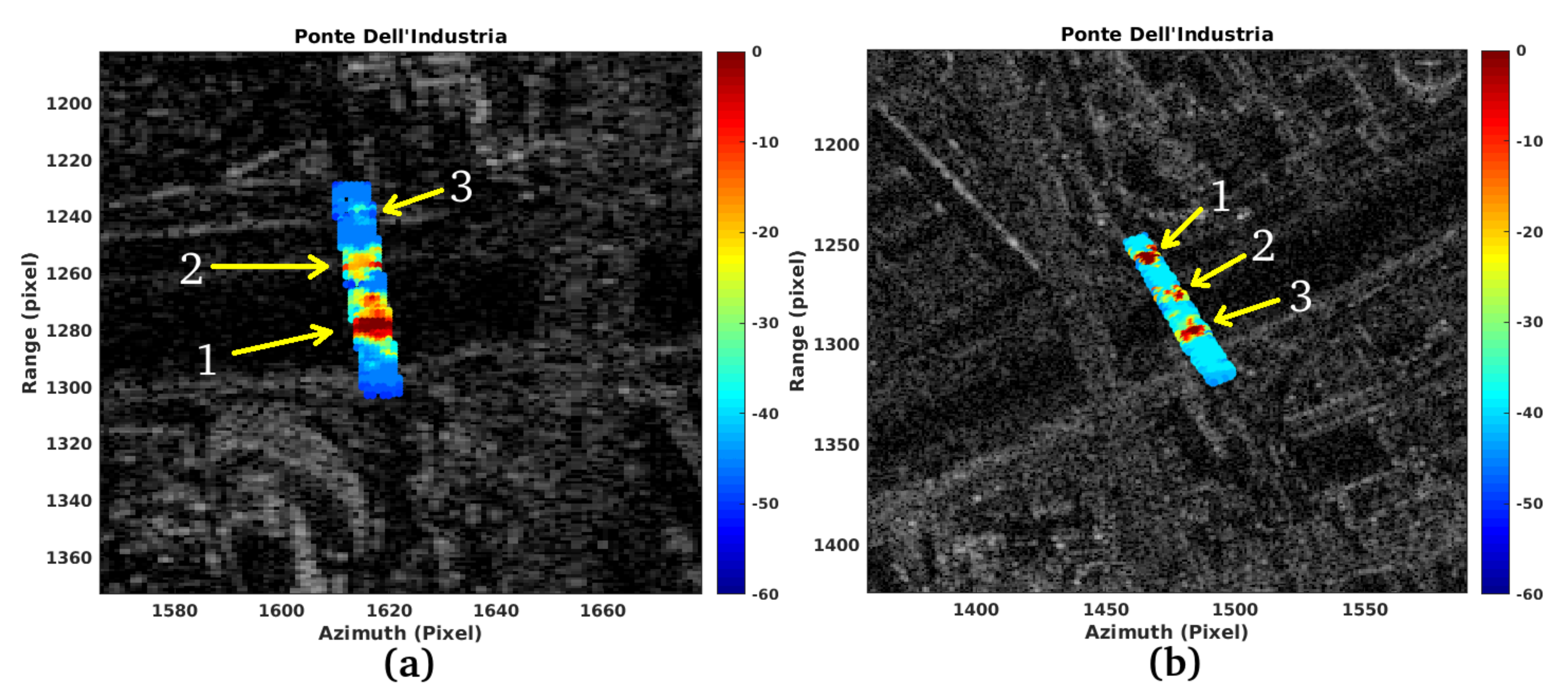
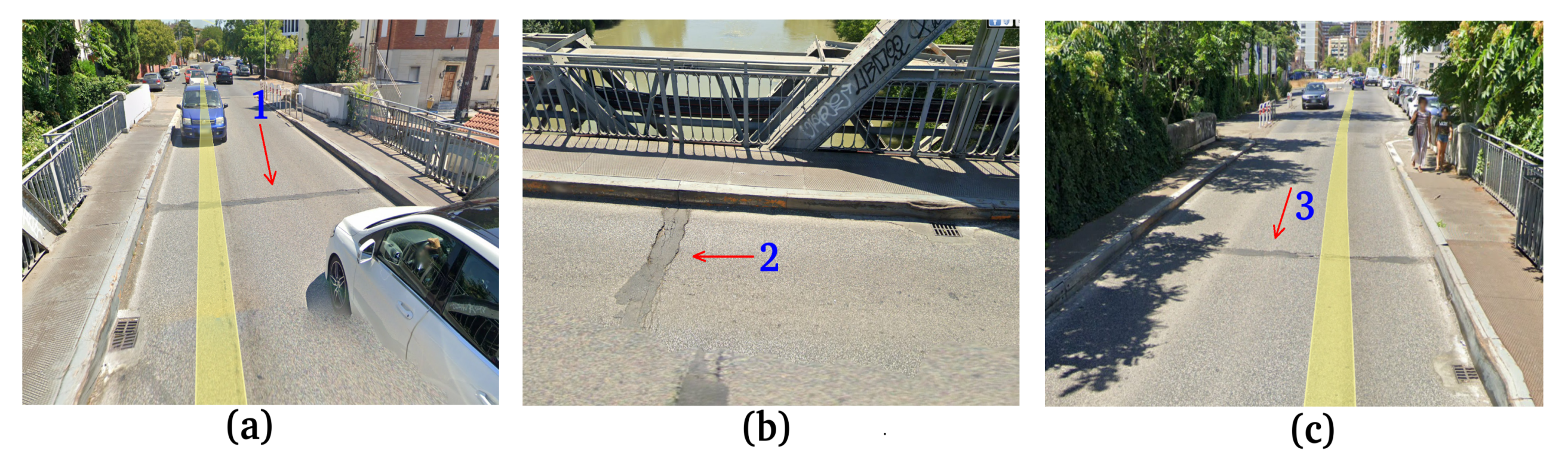
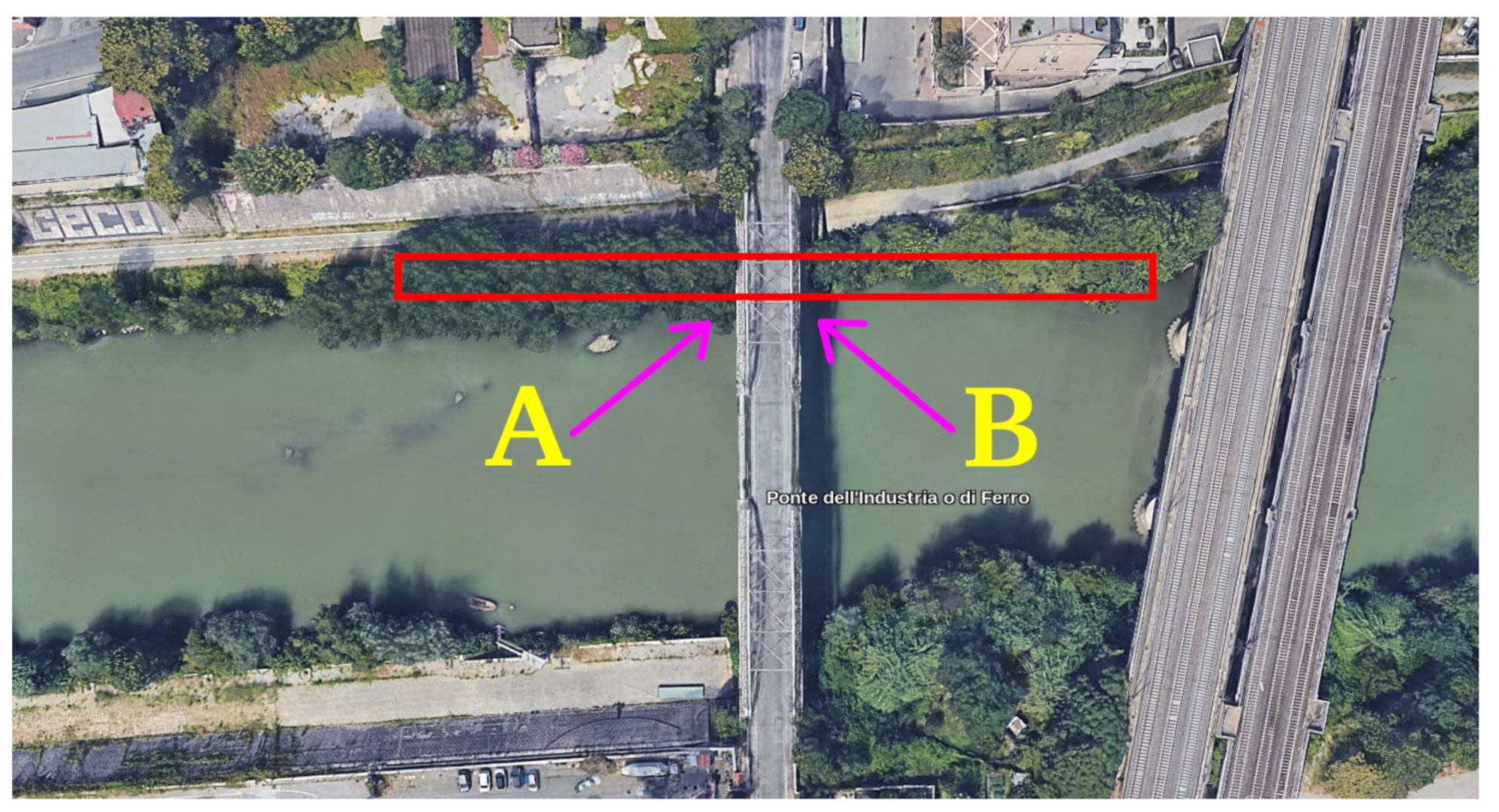
- “Ponte dell’Industria” is a bridge crossing the Tiber River when it flows through the city of Rome (in the analysis, we consider two opposite geometries, namely, right ascending and right descending, to compare different acquisitions over the same bridge and to prove the repeatability of the procedure);
- (2)
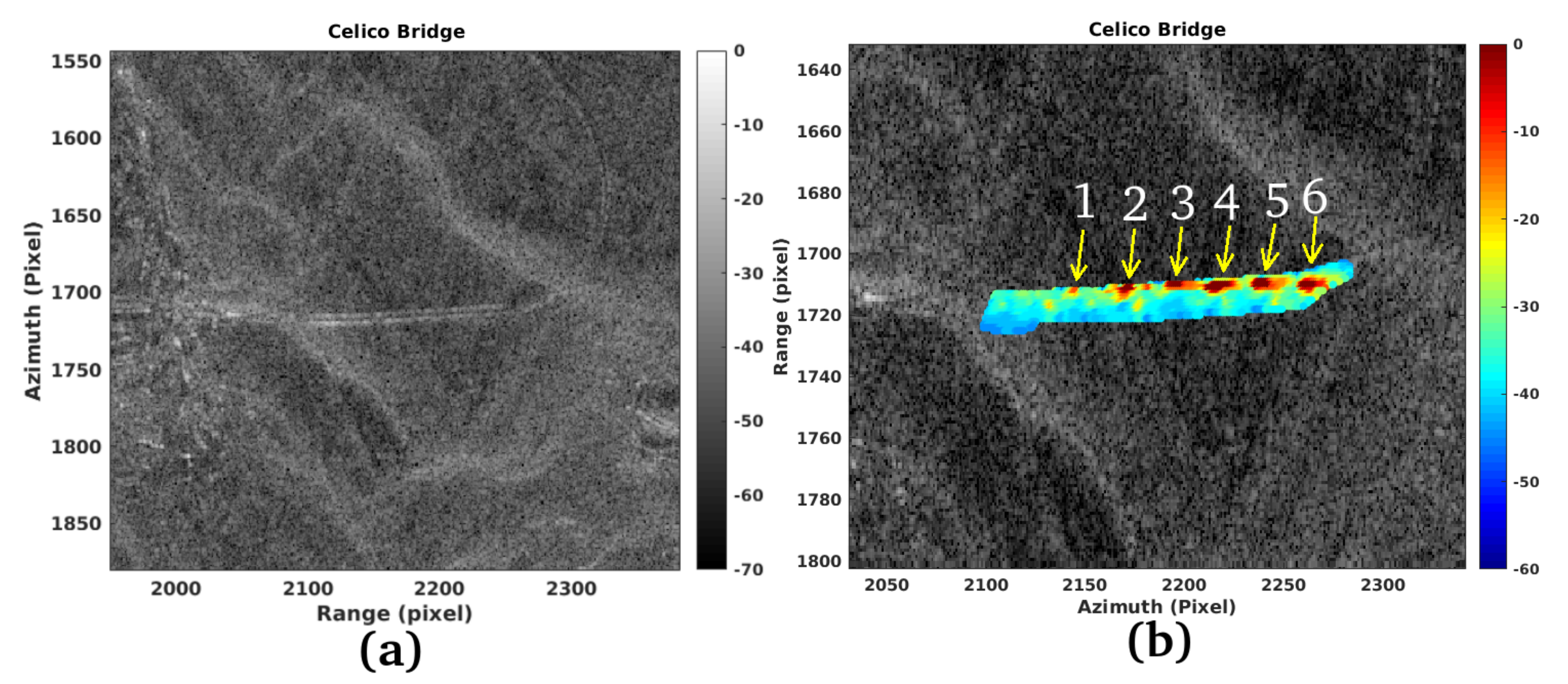
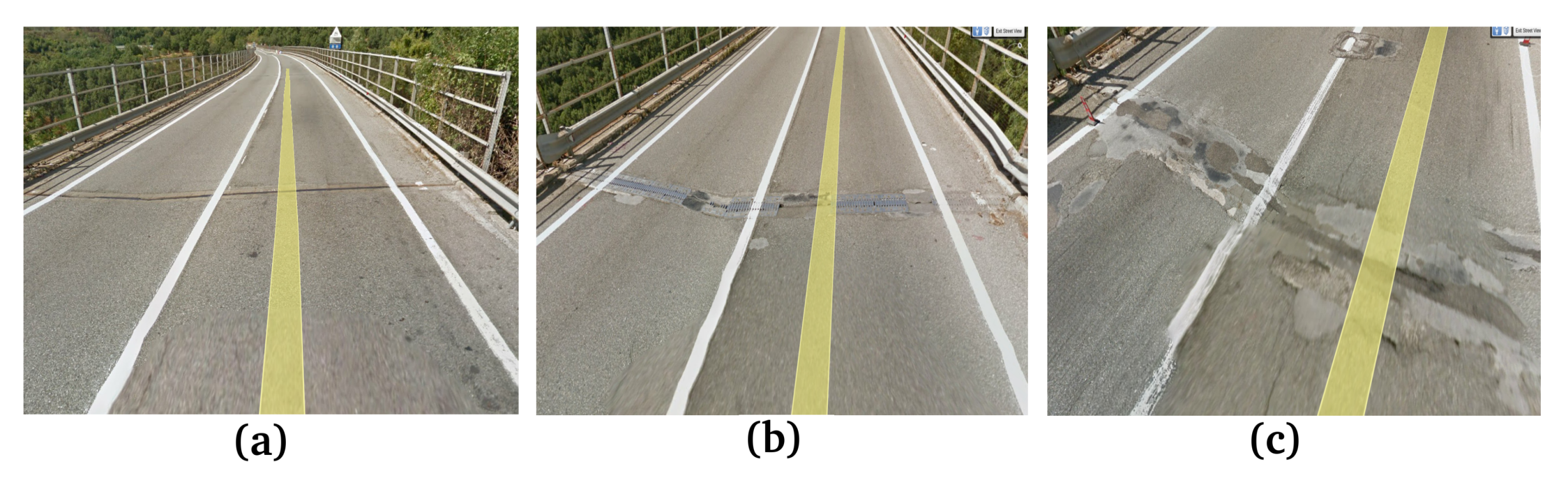
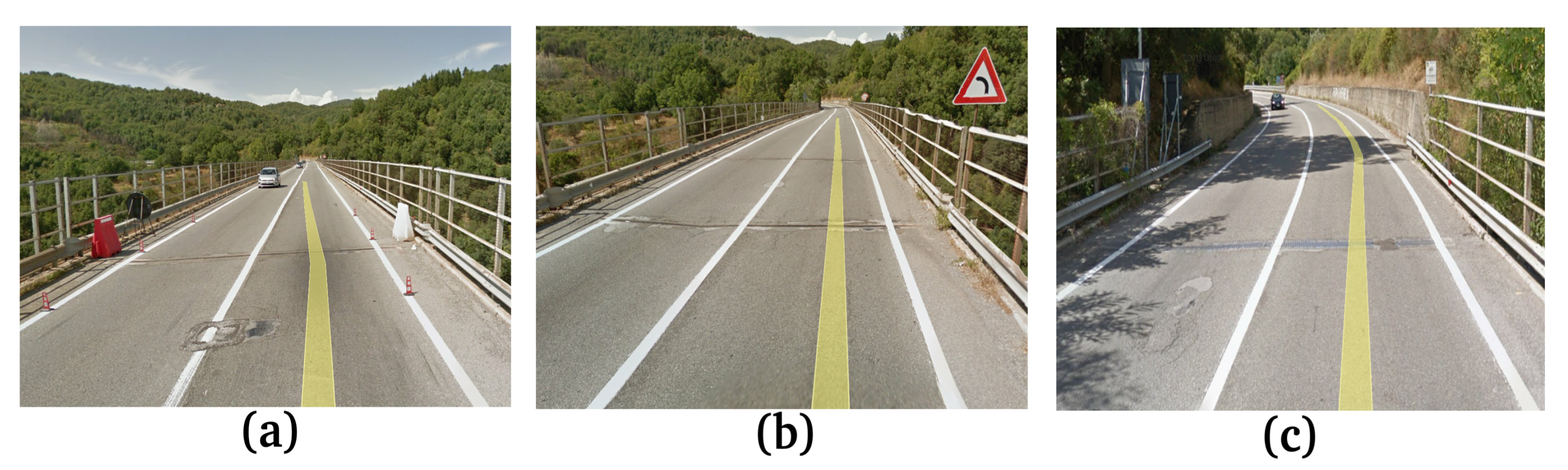
- “Celico” bridge is located in Calabria, a region in southern Italy (it consists of three main spans and two semi-arches);
- (3)
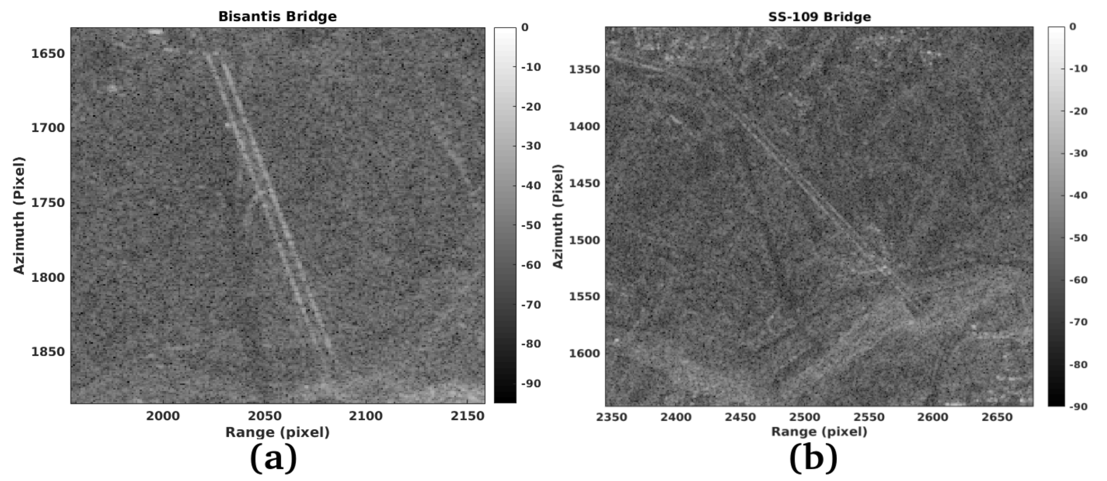
- “Bisantis” bridge is also located in Calabria (both Celico and Bisantis are made of pre-compressed concrete that are very old and still in operation today);
- (4)
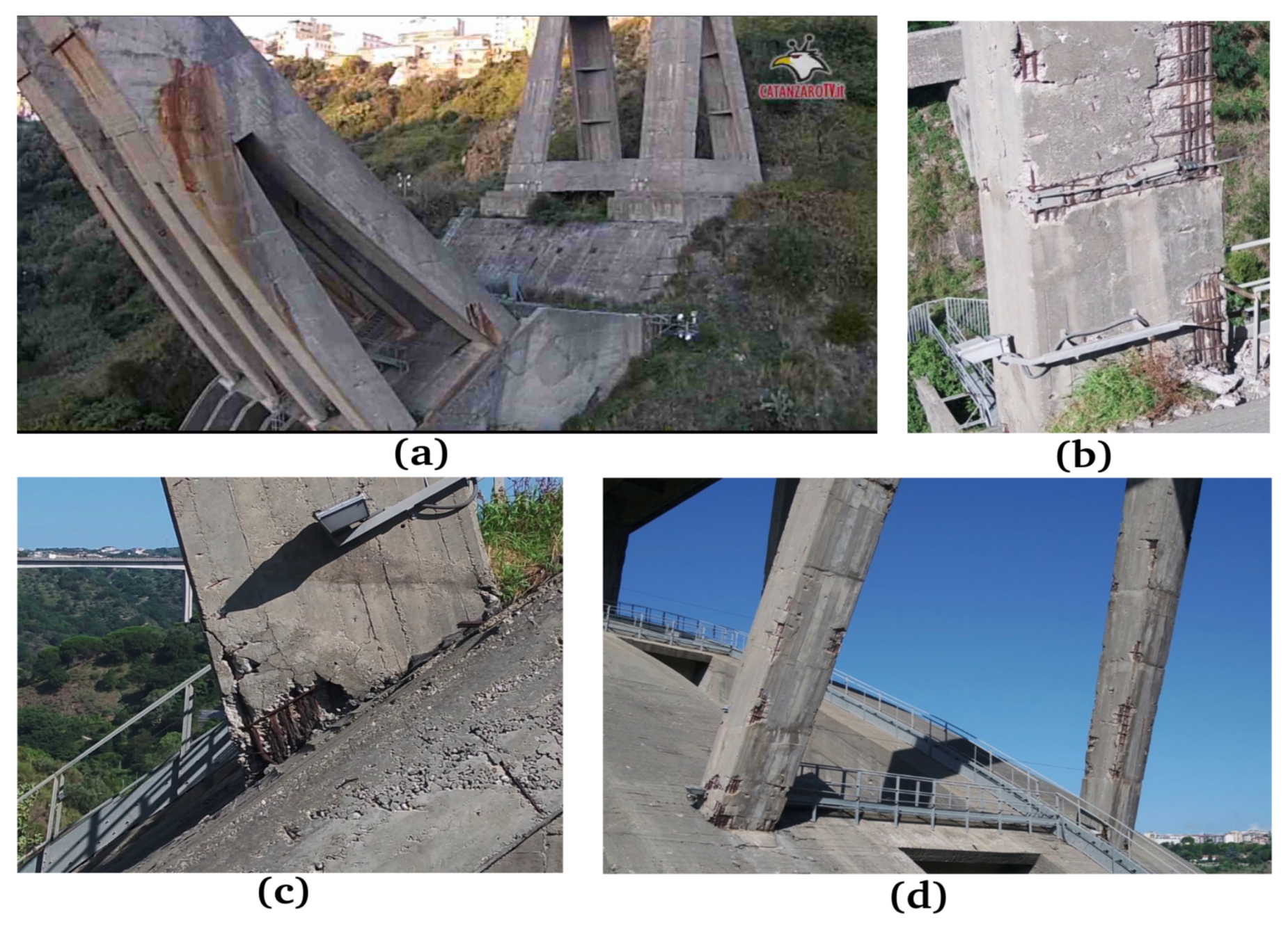
- “Italia” of the “SS-119”, an Italian motorway, is also located in Calabria region (the vibration anomalies are analysed);
- (5)
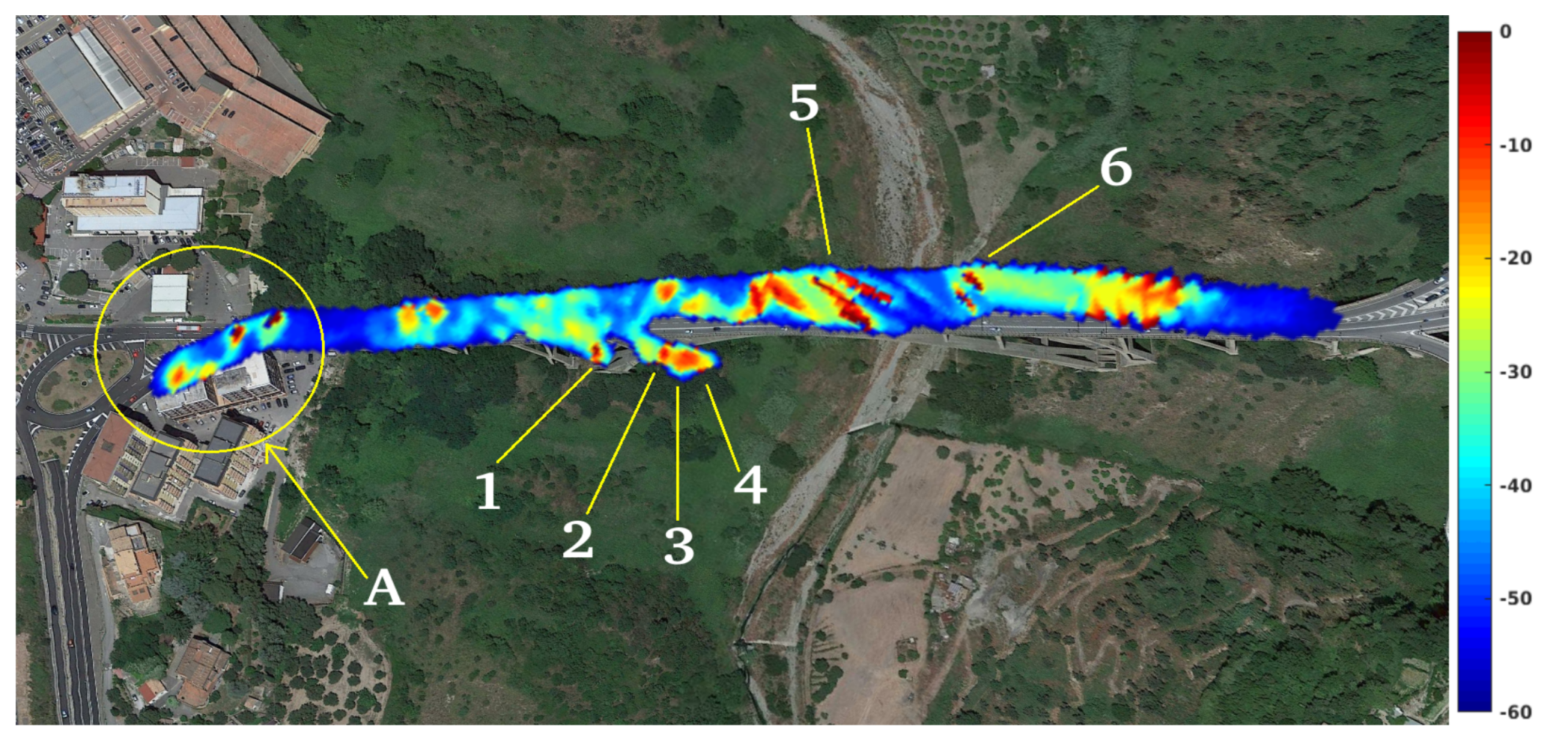
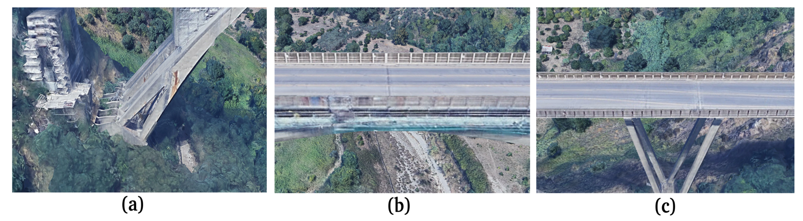
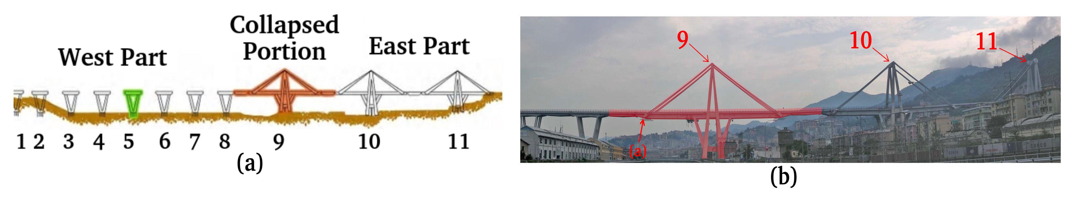
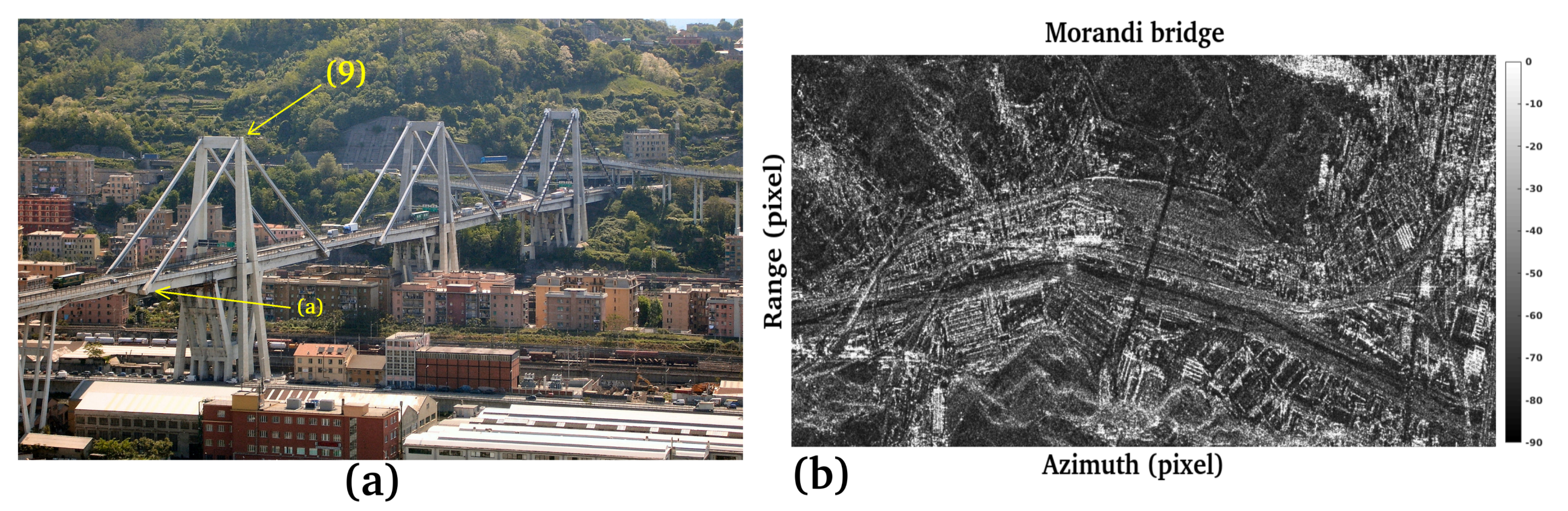
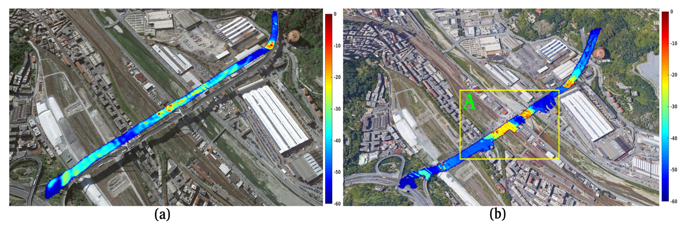
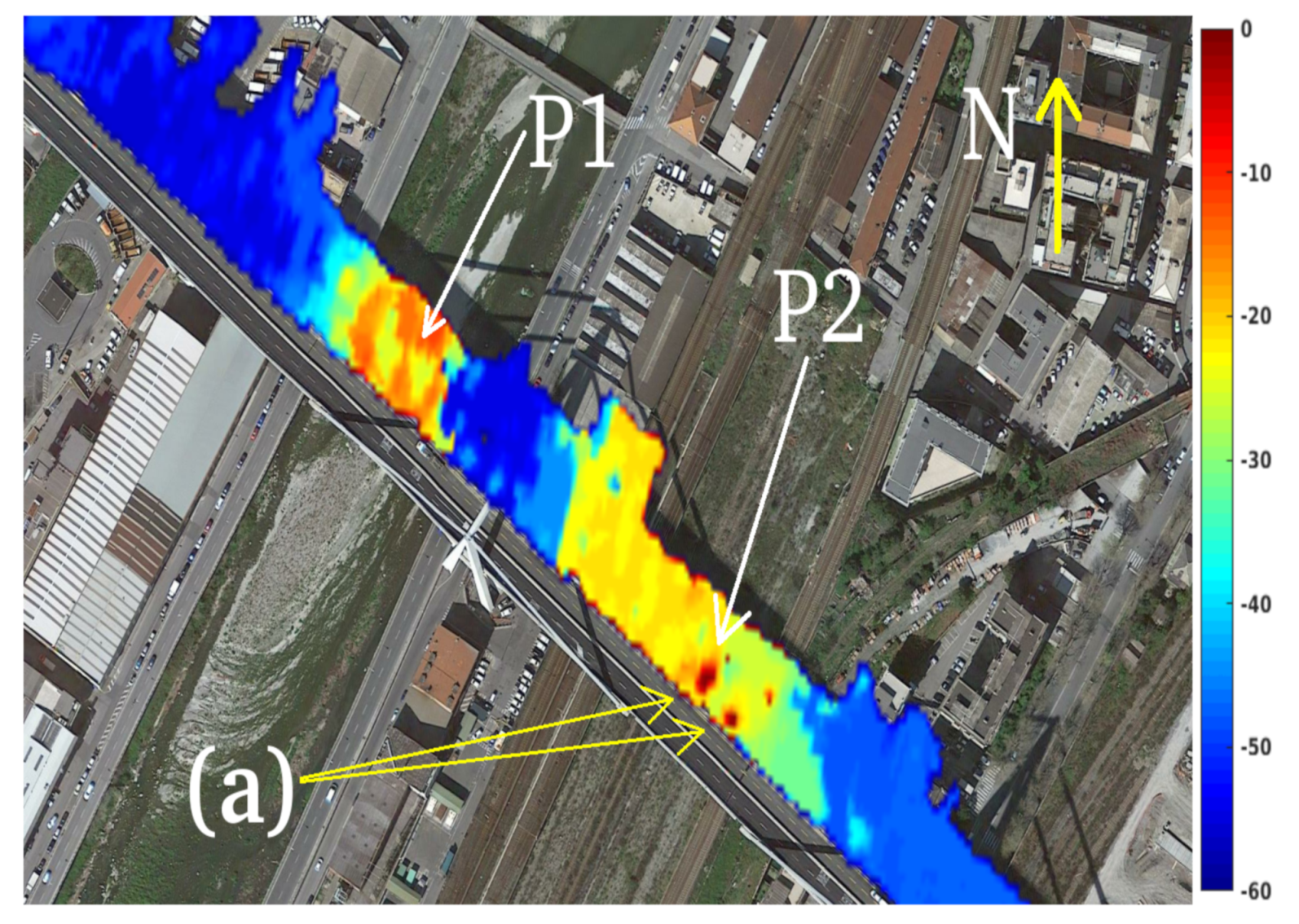
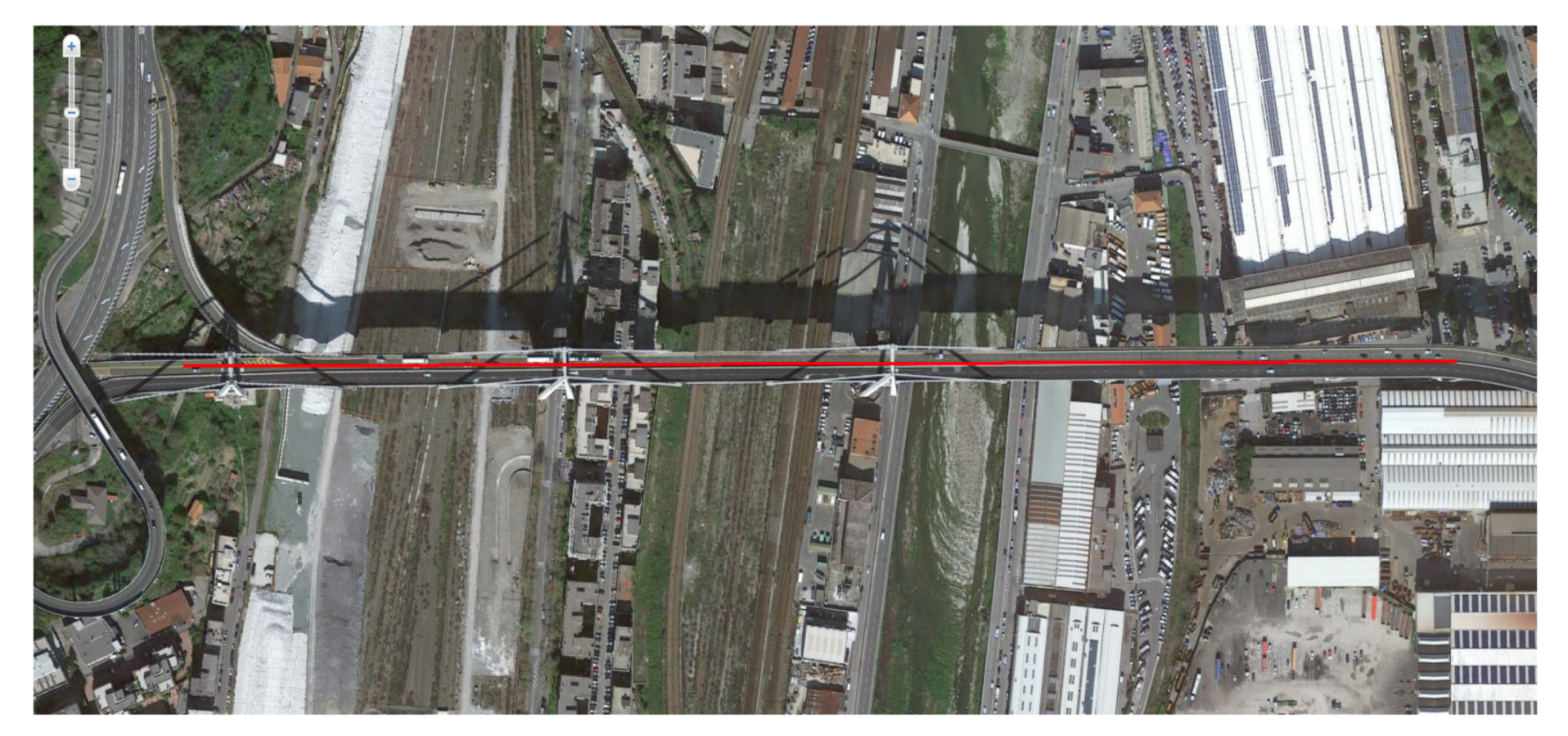
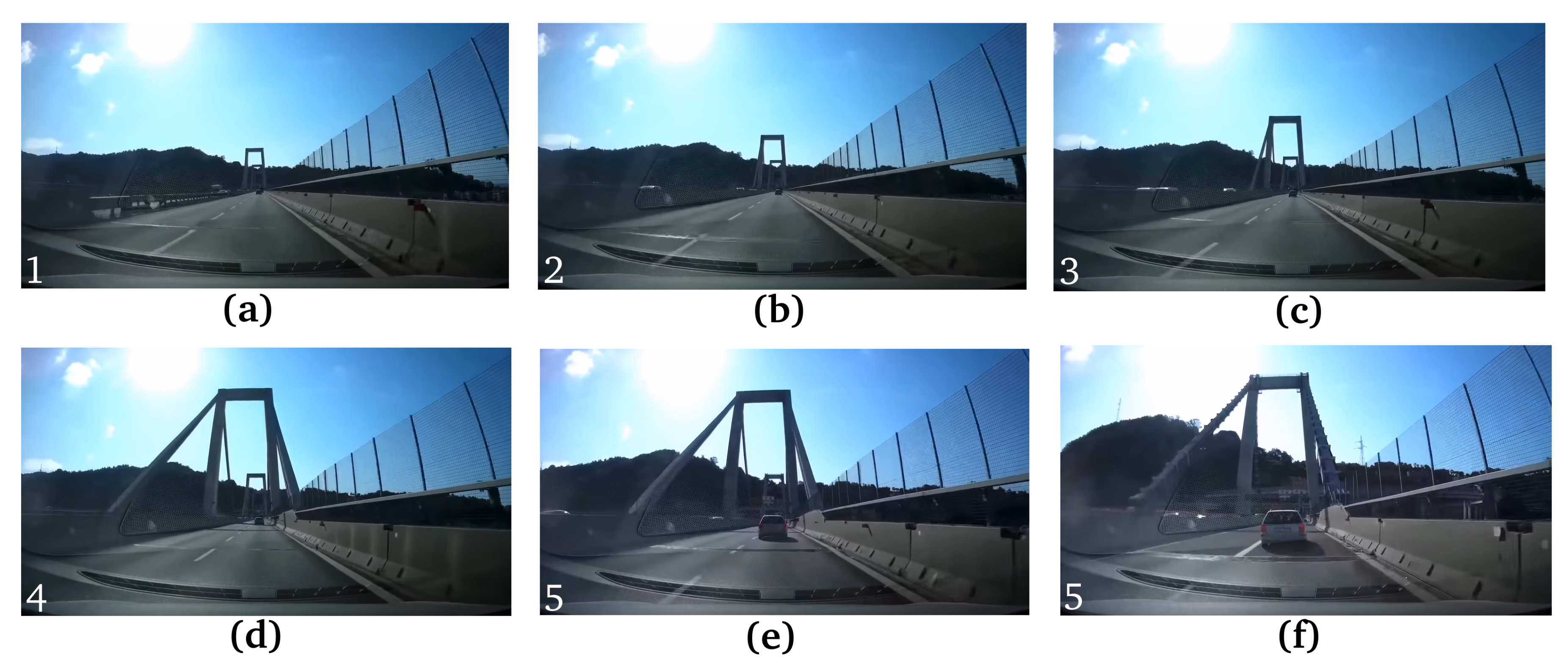
- the last case study investigates the vibration analysis of the the “Morandi” bridge, which collapsed during a strong storm on 14 August 2018 (the “Morandi” bridge crossed the city of Genoa and its collapse caused 43 victims, and, thanks to the proposed method, many critical points have been found on the collapsed stall in a period before the tragic event).
3.1. Study Case 1
3.2. Study Case 2
3.3. Study Case 3
3.4. Study Case 4
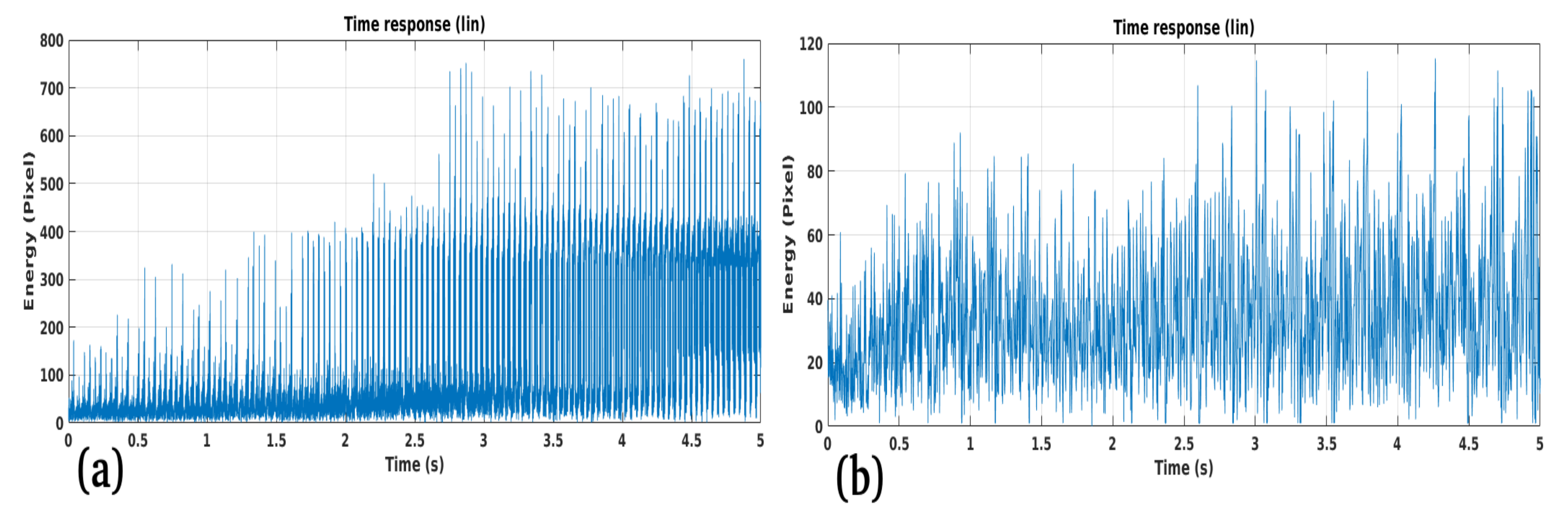
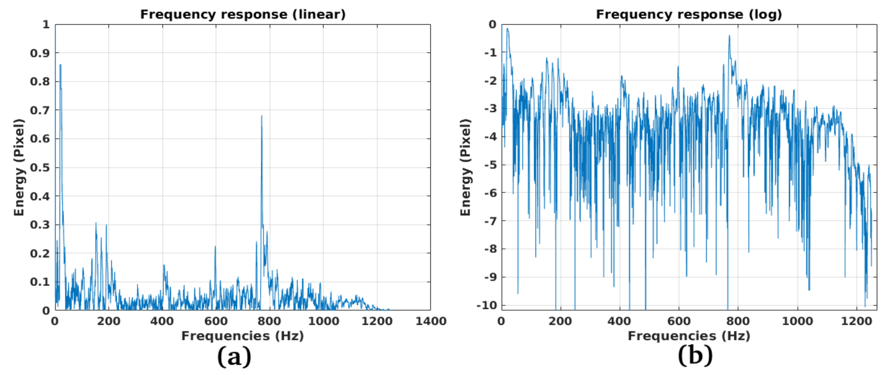
3.5. Study Case 5
4. Discussion
5. Conclusions
Author Contributions
Funding
Acknowledgments
Conflicts of Interest
References
- Chen, H.P.; Ni, Y.Q. Structural Health Monitoring of Large Civil Engineering Structures; Wiley Blackwell: Hoboken, NJ, USA, 2018. [Google Scholar]
- Scott, C.P.; Lohman, R.B.; Jordan, T.E. InSAR constraints on soil moisture evolution after the March 2015 extreme precipitation event in Chile. Sci. Rep. 2017, 7, 1–9. [Google Scholar] [CrossRef] [PubMed]
- Bekaert, D.P.S.; Hamlington, B.D.; Buzzanga, B.; Jones, C.E. Spaceborne Synthetic Aperture Radar Survey of Subsidence in Hampton Roads, Virginia (USA). Sci. Rep. 2017, 7, 14752. [Google Scholar] [CrossRef] [PubMed]
- Burnol, A.; Aochi, H.; Raucoules, D.; Veloso, F.M.L.; Koudogbo, F.N.; Fumagalli, A.; Chiquet, P.; Maisons, C. Wavelet-based analysis of ground deformation coupling satellite acquisitions (Sentinel-1, SMOS) and data from shallow and deep wells in Southwestern France. Sci. Rep. 2019, 9, 4903. [Google Scholar] [CrossRef] [PubMed]
- Carlà, T.; Intrieri, E.; Raspini, F.; Bardi, F.; Farina, P.; Ferretti, A.; Colombo, D.; Novali, F.; Casagli, N. Perspectives on the prediction of catastrophic slope failures from satellite InSAR. Sci. Rep. 2019, 9, 1–9. [Google Scholar] [CrossRef] [PubMed]
- Sousa, J.J.; Ruiz, A.M.; Bakoň, M.; Lazecky, M.; Hlaváčová, I.; Patrício, G.; Delgado, J.M.; Perissin, D. Potential of C-Band SAR Interferometry for Dam Monitoring. Procedia Comput. Sci. 2016, 100, 1103–1114. [Google Scholar] [CrossRef]
- Lazecky, M.; Perissin, D.; Bakon, M.; De Sousa, J.M.; Hlavacova, I.; Real, N. Potential of satellite InSAR techniques for monitoring of bridge deformations. In Proceedings of the 2015 Joint Urban Remote Sensing Event (JURSE), Lausanne, Switzerland, 30 March–1 April 2015; pp. 1–4. [Google Scholar]
- Ullo, S.L.; Addabbo, P.; Di Martire, D.; Sica, S.; Fiscante, N.; Cicala, L.; Angelino, C.V. Application of DInSAR Technique to High Coherence Sentinel-1 Images for Dam Monitoring and Result Validation Through In Situ Measurements. IEEE J. Sel. Top. Appl. Earth Obs. Remote Sens. 2019, 12, 875–890. [Google Scholar] [CrossRef]
- De Corso, T.; Mignone, L.; Sebastianelli, A.; Del Rosso, M.P.; Yost, C.; Ciampa, E.; Pecce, M.; Sica, S.; Ullo, S.L. Application of DInSAR technique to high coehrence satellite images for strategic infrastructure monitoring. In Proceedings of the 2020 IEEE International Geoscience and Remote Sensing Symposium, Waikoloa, HI, USA, 19–24 July 2020. [Google Scholar]
- Ferretti, A.; Prati, C.; Rocca, F. Nonlinear subsidence rate estimation using permanent scatterers in differential SAR interferometry. IEEE Trans. Geosci. Remote Sens. 2000, 38, 2202–2212. [Google Scholar] [CrossRef]
- Ferretti, A.; Prati, C.; Rocca, F. Permanent scatterers in SAR interferometry. IEEE Trans. Geosci. Remote Sens. 2001, 39, 8–20. [Google Scholar] [CrossRef]
- Biondi, F.; Clemente, C.; Orlando, D. An Atmospheric Phase Screen Estimation Strategy Based on Multichromatic Analysis for Differential Interferometric Synthetic Aperture Radar. IEEE Trans. Geosci. Remote Sens. 2019, 57, 7269–7280. [Google Scholar] [CrossRef]
- Fujino, Y. Vibration, control and monitoring of long-span bridges—Recent research, developments and practice in Japan. J. Constr. Steel Res. 2002, 58, 71–97. [Google Scholar] [CrossRef]
- Li, H.; Laima, S.; Zhang, Q.; Li, N.; Liu, Z. Field monitoring and validation of vortex-induced vibrations of a long-span suspension bridge. J. Wind Eng. Ind. Aerodyn. 2014, 124, 54–67. [Google Scholar] [CrossRef]
- Biondi, F.; Addabbo, P.; Clemente, C.; Ullo, S.; Orlando, D. Monitoring of Critical Infrastructures by Micro-Motion Estimation: the Mosul Dam Destabilization. IEEE J. Sel. Top. Appl. Earth Obs. Remote. Sens. 2020, 13, 6337–6351. [Google Scholar] [CrossRef]
- Curlander, J.C.; McDonough, R.N.; Soumekh, M. Synthetic Aperture Radar Signal Processing; Wiley: New York, NY, USA, 1991; Volume 7. [Google Scholar]
- Raney, R.K. Synthetic Aperture Imaging Radar and Moving Targets. IEEE Trans. Aerosp. Electron. Syst. 1971, AES-7, 499–505. [Google Scholar] [CrossRef]
- Ismail, F.; Ibrahim, A.; Martin, H. Identification of fatigue cracks from vibration testing. J. Sound Vib. 1990, 140, 305–317. [Google Scholar] [CrossRef]
- Cheng, S.M.; Swamidas, A.S.J.; Wu, X.J.; Wallace, W. Vibrational Response of a Beam with a Breathing Crack. J. Sound Vib. 1999, 225, 201. [Google Scholar] [CrossRef]
- Ballo, I. Non-linear effects of vibration of a continuous transverse cracked slender shaft. J. Sound Vib. 1998, 217, 321–333. [Google Scholar] [CrossRef]


| SAR Parametrer | Value |
|---|---|
| Chirp bandwidth | 80 MHz |
| PRF | 2.5 kHz |
| PRT | 0.23 ms |
| Antenna length | 6 m |
| Type of acquisition | Stripmap |
| Polarization | HH |
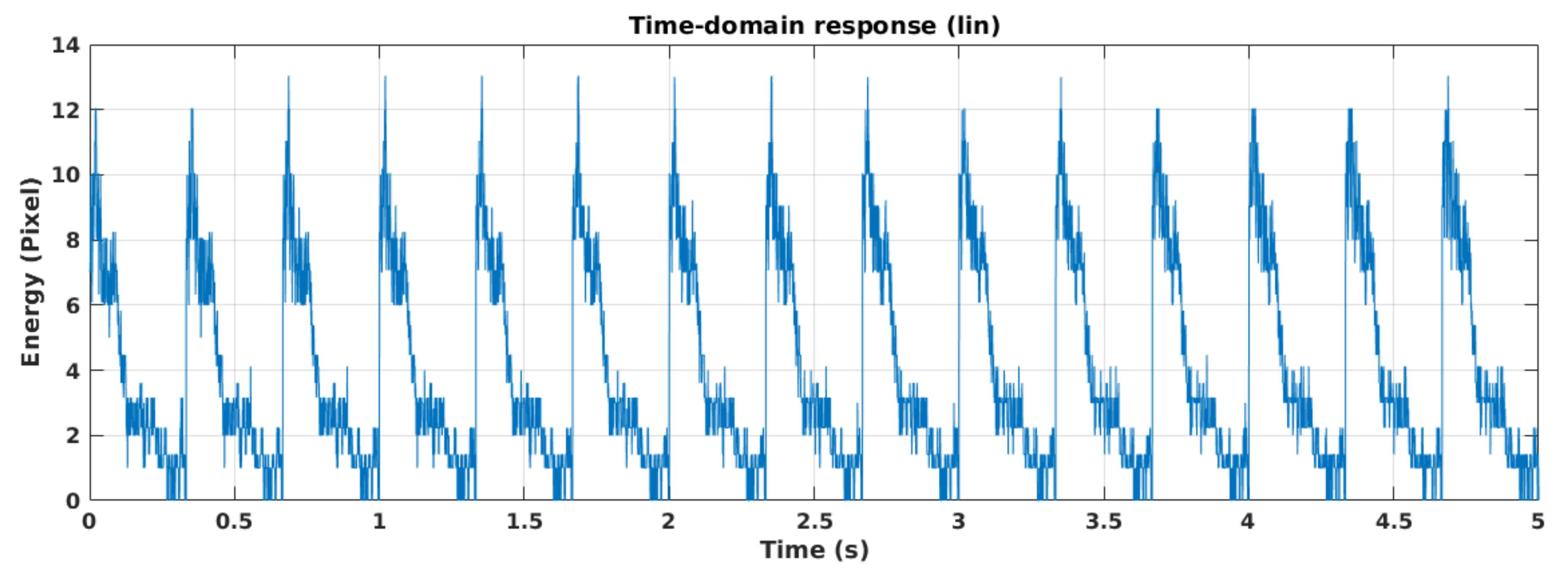
| Acquisition duration | 5 s |
| Platform velocity | 7 km/s |
| Observation height | 650,000 m |
| Case Study | Bridge Name | Processing | Coordinates (WGS-84) | Time of obs. | Number of obs. |
|---|---|---|---|---|---|
| 1 | Industria | Modal | 41°52′18.96″ N | 8 March–13 March 2018 | 2 |
| 12°28′19.89″ E | |||||
| 2 | Celico | Modal | 39°18′49.84″ N | 21 March 2018 | 1 |
| 16°20′64.89″ E | |||||
| 3 | Bisantis | Modal | 38°54′34.11″ N | 12 April 2018 | 1 |
| 16°35′24.15″ E | |||||
| 4 | Italia | Modal | 38°54′66.11″ N | 14 March 2018 | 1 |
| 16°34′35.15″ E | |||||
| 5 | Morandi | Modal | 44°25′33.11″ N | 21 January 2016–5 July 2018 | 2 |
| 08°53′18.15″ E |
Publisher’s Note: MDPI stays neutral with regard to jurisdictional claims in published maps and institutional affiliations. |
© 2020 by the authors. Licensee MDPI, Basel, Switzerland. This article is an open access article distributed under the terms and conditions of the Creative Commons Attribution (CC BY) license (http://creativecommons.org/licenses/by/4.0/).
Share and Cite
Biondi, F.; Addabbo, P.; Ullo, S.L.; Clemente, C.; Orlando, D. Perspectives on the Structural Health Monitoring of Bridges by Synthetic Aperture Radar. Remote Sens. 2020, 12, 3852. https://doi.org/10.3390/rs12233852
Biondi F, Addabbo P, Ullo SL, Clemente C, Orlando D. Perspectives on the Structural Health Monitoring of Bridges by Synthetic Aperture Radar. Remote Sensing. 2020; 12(23):3852. https://doi.org/10.3390/rs12233852
Chicago/Turabian StyleBiondi, Filippo, Pia Addabbo, Silvia Liberata Ullo, Carmine Clemente, and Danilo Orlando. 2020. "Perspectives on the Structural Health Monitoring of Bridges by Synthetic Aperture Radar" Remote Sensing 12, no. 23: 3852. https://doi.org/10.3390/rs12233852
APA StyleBiondi, F., Addabbo, P., Ullo, S. L., Clemente, C., & Orlando, D. (2020). Perspectives on the Structural Health Monitoring of Bridges by Synthetic Aperture Radar. Remote Sensing, 12(23), 3852. https://doi.org/10.3390/rs12233852