Efficient Marginalized Particle Smoother for Indoor CSS–TOF Localization with Non-Gaussian Errors

Abstract

The time-series state and parameter estimations of indoor localization continue to be a topic of growing importance. To deal with the nonlinear and positive skewed non-Gaussian dynamic of indoor CSS–TOF (Chirp-Spread-Spectrum Time-of-Flight) ranging measurements and position estimations, Monte Carlo Bayesian smoothers are promising as involving the past, present, and future observations. However, the main problems are how to derive trackable smoothing recursions and to avoid the degeneracy of particle-based smoothed distributions. To incorporate the backward smoothing density propagation with the forward probability recursion efficiently, we propose a lightweight Marginalized Particle Smoother (MPS) for nonlinear and non-Gaussian errors mitigation. The performance of the position prediction, filtering, and smoothing are investigated in real-world experiments carried out with vehicle on-board sensors. Results demonstrate the proposed smoother enables a great tool by reducing temporal and spatial errors of mobile trajectories, with the cost of a few sequence delay and a small number of particles. Therefore, MPS outperforms the filtering and smoothing methods under weak assumptions, low computation, and memory requirements. In the view that the sampled trajectories stay numerically stable, the MPS form is validated to be applicable for time-series position tracking.

1. Introduction

Indoor wireless positioning has attracted much attention in recent years, which is the key important issue arising in robotics, advanced signal processing, social networking, or mobile monitoring of indoor environments, just to mention a few. Most positioning applications provide time-series measurements and demand for continuous estimation of the target’s position [1]. Particularly, when considering Time-of-Flight (TOF) measurements as ranging measurements, the uncertainty of ranging measurements is coherent with dynamic environments and sensor limitations [2]. Due to that, the indoor positioning problem is to understand the dynamic of which limited and noisy observations are available. In the main, a considerable amount of research has been put into the purpose of sequential estimations of indoor position, also known as indoor sequential positioning or position tracking [3,4,5].

Although fairly fruitful research has been proposed in sequential positioning algorithms, to achieve accurate indoor position tracking from a multimodal distribution or noisy measurements is still very challenging due to the following difficulties:

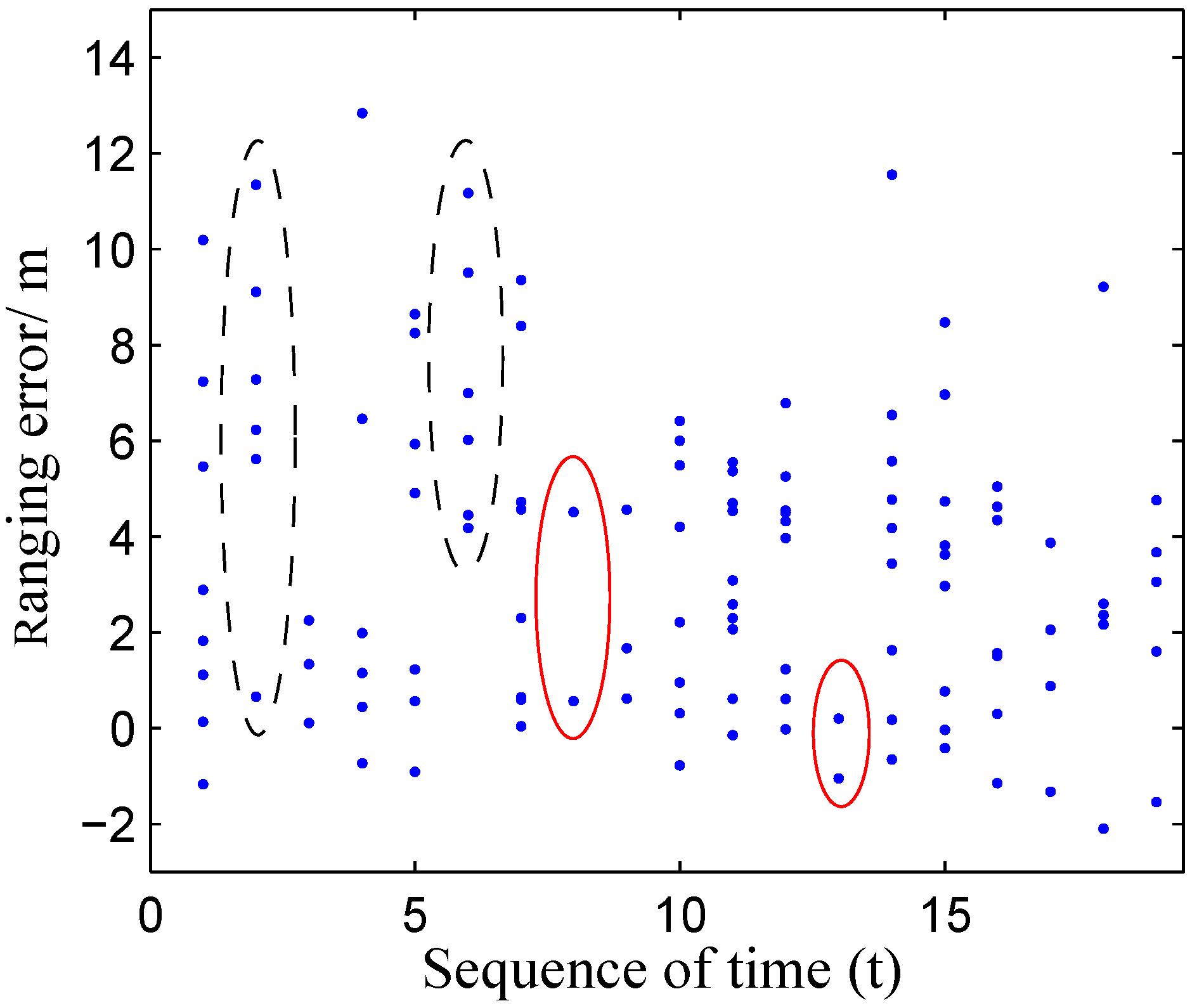
• Indoor RF ranging uncertainty. Wireless ranging technique is a convenient solution for indoor positioning and tracking, but suffering from severe uncertainty of radio frequency (RF) measurements. Thus, the probability density taking into account more observations may not necessarily lead to better accuracy.
• Nonlinear/non-Gaussian dynamic. People or a mobile device can usually take non-uniform and heterogeneous motions, which are difficult to model. Furthermore, indoor RF ranging error is verified to be non-Gaussian in both simulations [6,7] and real-world experiments [8,9,10]. Hence, both the observation and state transition are prone to be nonlinear and/or non-Gaussian problems, that the closed-form solution often does not exist.
• Priori knowledge. The implementation and performance of the Bayesian framework depend on the priori knowledge of the measurement noise and process models, whereas the prior information is often not accurate.
• Computation, real-time and implementation constraints. To be practical, such a sequential tracking solution should be efficient in computation, time delay, and implementation.
  • Portable devices are typically resources limited, i.e., computing, storage, and communication, etc. Hence, the problem, in using in mobile positioning, is the large storage and computation requirement. Therefore, the objective is to optimize the estimation density for continuous trajectories.
  • Near real-time position tracking is imposed by a tight delay constraint in the order of milliseconds [11,12]. State estimations require to investigate the entire sequence of the observations and state, which are time-consuming; also, the performance of fixed-Lag smoothing is dependent on the size of the smoothing lag ($△T$) [13].
• Instability. It is well known that wireless network resources are scarce and time-varying. Thus, the smoothed tracking has to be robust to the problems of sparse measurements, inconsistent measurements or even losing tracking.

For sequential positioning, the family of recursive Bayesian methods have been subject to extensive research in literature, i.e., the sequential Bayesian filtering and smoothing methods in Hidden Markov Chain (HMC) framework [14,15,16,17]. Bayesian filtering estimates the state by updating recursively with every new incoming measurement, by applying the time-sequential hidden Markov process as a broad class of Kalman filters [18] or particle filters (also known as sequential Monte Carlo (MC) methods) [19]. The framework of filtering is defined as the estimation of the state at the same time as the current measurement. However, in the context of indoor positioning, there is frequent absences of radio measurements. Then, the Kalman filter works only in prediction mode, which degrades the prediction accuracy rapidly with time.

Recently, smoothing has attracted attention mainly in indoor position tracking. In contrast to normal filtering recursions, the smoothing frame is of particular interest as being able to make the state probability from not only the past and present observations (${\mathbf{z}}_{1:t}$) but also future observations (${\mathbf{z}}_{t:T}$, $t<T$) [20]. The smoothing methods all fall into one of the two categories: joint or marginal. The early surveys have studied the possibilities of smoothing in a Bayesian framework [21,22,23,24], i.e., the Rauch-Tung-Striebel (RTS) smoothing algorithm [25] presented by Rauch, Tung and Striebel, the Forward Filtering Backward Smoothing (FFBS) [26] by Kitagawa and the Two-Filter smoother (TFS) [27] by Fraser and Potter, and the One Time-step Particle Smoothing by Yuan and Huaming [28]. Essentially, these smoothing frames tend to achieve improvements of time series analysis by involving the information of more observations. The above smoothing frames can be obtained by recursive formulas, i.e., the Kalman smoother [29,30], the extended Kalman smoother [31], the unscented Kalman smoother [32], the Gaussian-sum methods [33]. On the other hand, sequential MC algorithms (known generically as particle smoother) [34], approximate the time series estimation by a set of weighted particles. The Kalman smoother is an optimal smoother. To reduce the complexity of particle smoothers, some literature [35] improve the computational complexity which is linear to the number of particles. Furthermore, thanks to massive increases in the computational power of mobile devices, some of these smoothing methods and their variations have been applied in embedded mobile positioning [36,37,38,39]. Based on these smoothing approaches, different solutions for non-linear sequential densities have been developed, e.g., Nurminen and Ristimaki deployed a fixed-interval forward–backward smoother to improve the position estimation for non-real-time applications [40]. Most of these methods involve the form of smoothing as an extension to the particle filter, which reweight particles to approximate the smoothing density based on the filter density. For further positioning error mitigation, more schemes can be explored, i.e., multiple observation sub-models [41], integration positioning [42], velocity/direction modeling [43], non-parametric models [44] and map matching [45] and etc.

Nevertheless, the key issues of applying a smoothing frame in RF position tracking are to derive tractable solutions to ameliorate the smoothing efficiency. To reduce the establishment cost and improve the accuracy, this paper focuses on implementing a smoothing frame with the observations after the present, namely, Marginalized Particle Smoother (MPS). Besides, the nonlinear and non-Gaussian 2D positioning recursion is not analytically solvable. Towards this end, we propose a lightweight MPS on a Sequential Monte Carlo (SMC) method. The proposed MPS hypothesizes that the smoothing density allows a better probability propagation, which continuously estimates the target’s position based on the posterior derived from the general smoothing density. In the scenarios of a relatively high modeling uncertainty of the experimental measurements and target’s motion, the results demonstrate that our proposed MPS is able to considerably improve the performance. In particular, the contribution of this study is summarized in the following.

• Implement a lightweight marginalized particle smoother (MPS) on the SMC frame, which provides a trackable solution to the nonlinear and non-Gaussian indoor range-based positioning.
• Propose the marginal smoothed smoothing that dynamically derives the posterior from a backward smoothing density in an efficient way. The virtue of MPS is that it can be applied to a very wide class of SMC methods.
• Implement two popular nonlinear smoothing solutions: Forward Filtering Backward Smoothing (FFBS) and Two-filter Smoothing (TFS).
• Combine two linear smoother (Moving Average (MA) smoother and Rauch-Tung-Striebel (RTS) smoother) with a nonlinear filtering output (Generic Particle Filter (GPF)).
• The aforementioned smoothing algorithms are evaluated over indoor CSS–TOF (Chirp-Spread-Spectrum Time-of-Flight) test-bed. Experimental results validate the effectiveness and efficiency of the MPS framework on real-world indoor position tracking.

The remainder of this paper is structured as follows. Section 2 presents the problem statement and system models. Section 3 introduces the Bayesian smoothing formulas of FFBS, TFS, and MPS in detail. The moving average and Kalman smoother are introduced in Section 4. The performance evaluation of real-world indoor tracking experiments are provided in Section 5. Section 6 concludes this work.

2. Motivation and Problem Statement

2.1. Motivation

In RF range-based positioning, either the ranging that sensors measure or the motion of the target are usually difficult to model accurately. The mobile device can behave non-uniform and heterogeneous motions (i.e., stopping, going forward, backing, turning, or jumping to another site, etc.). In addition, the positioning instability arises from the lack of LOS (Line-of-sight) measurements. The experimental results [6,46] reveal that the ranging error observes a large variance, due to system noise, multi-path effect, Non-line-of-sight (NLOS) propagations, unknown wireless interference, and system noise, etc. In the context of sequential estimations, recursive Bayesian methods are the most widely-used strategy to combat the modeling uncertainty, i.e., Bayesian filtering or smoothing methods. Filtering represents the posterior ($p\left({\mathbf{x}}_t\right|{\mathbf{z}}_{1:t})$) of the current state given the observations up to the current time t; smoothing corresponds to the state density ($p\left({\mathbf{x}}_t\right|{\mathbf{z}}_{1:T})$) based on all of the observations up to some later time ($T,t+1\le T$). Compared with filtering, smoothing tends to yield more informative state estimates as taking ${\mathbf{z}}_T$ into account.

To generate a smooth representation of the mobile trajectory, Bayesian smoothing methods have been presented and used in state estimation [47]. Some of them are generally put forward: the fixed-interval sequential smoother, the fixed-lag smoother, the forward–backward smoother, and the two-filter smoother. They are derived using different strategies to solve either the joint or the marginal smoothing problem. Overall, the experiment results validate that the smoothing frame can be effective in real indoor tracking. We summarize that: (1) the observation a few time-series later (${\mathbf{z}}_T$) contains a significant amount of information to combat the state uncertainty and the measurement errors; (2) the MPS improvement arises from incorporating the smoothing density into the SMC recursion, differing from the referral smoothing algorithms that only influence the backward density. The smoothing methods are beneficial by deriving the state probability from the past, present, and future observations, which generally provide better approximations of marginal smoothing distributions compared with filtering methods [48,49].

Besides the smooth representation of the tracking trajectory, the smoothing frame is more useful for a relatively small number of indoor ranging observations. It is defined as a sparsity problem of LOS ranging observations, which is categorized into two types:

• Sparse anchors or missing measurements: the number of ranging measurements is insufficient due to the sparse anchor deployment or temporary packet loss;
• NLOS scenarios: there are enough ranging measurements, but the LOS measurements are the minority.

Figure 1 depicts the sparsity problem, indicating that it only occurs in a few ranging instances, e.g., the ranging neighboring the time-sequence with scarce measurements can still obtain sufficient measurements; moreover, the NLOS errors appear randomly rather than presenting continuously. Therefore, the sparsity problem is a temporary problem.

Generally, for non-sequential positioning, the sparsity problem can be alleviated by data fusion after waiting for more measurements. On the other hand, the smoothing frame of sequential position estimation is likely to mitigate the sparse problem, as it computes the state by conditioning not only on the observations up to current time but also on future ones.

2.2. Problem Statement

The Bayesian smoothing approaches provide a flexible framework for both smoothing the tracking trajectory and solving the sparsity problem in nonlinear time series. The smoothing density handles a time series state estimation given past, present and future observation

$$p\left({\mathbf{x}}_t\right|{\mathbf{z}}_{1:T}),$$

(1)

where $t+1\le T$. In the case that the time-series size of future observations is fixed, it is called as the smoothing lag

$$△T=T-t.$$

(2)

To apply the smoothing frame for fast range-based positioning, the challenge is twofold:

• Problem 1: Tractable solution
  For 2D range-based positioning, it cannot typically generate an analytical solution to the nonlinear and non-Gaussian models. Particle methods (Monte Carlo methods) [50] offer an approximate solution, unfortunately, they are intractable if the sample size is large.
• Problem 2: Implementation issue
  If the smoothing recursion involves the observations many time-series ahead ($t\ll T$), it can be computation, storage, and time-consuming. In other words, it is impractical to obtain overall smoothed estimates using the observations from the beginning to the end.

To summarize, given the available observations, filtering focuses on the current state, whereas smoothing focuses on the past states, and predicting focuses on future states. The closed-form solution for range-based positioning often does not exist, which is generally necessary to resort to Monte Carlo sampling methods. Sequential Monte Carlo with importance sampling [51] solves problems 1, which provides efficient solutions for nonlinear smoothing. However, the performance and applicability of a smoothing framework greatly depend on how much and how future observations are incorporated. Aiming at fast position tracking, it is preferable to formulate the smoothing density from the observations a few time-series ahead. Overall, we are interested in the smoothing density employing future time-series recursion ($p\left({\mathbf{x}}_t\right|{\mathbf{z}}_{1:T})$) on SMC.

3. Filtering and Smoothing

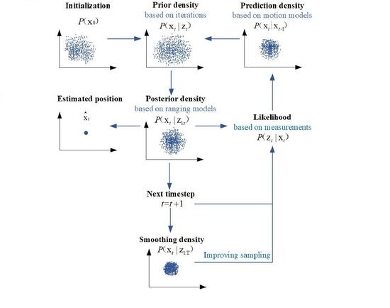
The sequential position estimation or position tracking is defined as the time-series estimation of the posterior given all available observations. The 2D position can be estimated by either filtering or smoothing frames.

• Filtering $p\left({\mathbf{x}}_t\right|{\mathbf{z}}_{1:t})$: to estimate the distribution of the state ${\mathbf{x}}_t$ conditionally to the observations up to t.
• Smoothing $p\left({\mathbf{x}}_t\right|{\mathbf{z}}_{1:T})$: to estimate the distribution of the state ${\mathbf{x}}_t$ conditionally to the observations up to T (with $t<T$).

To smooth the estimated trajectory, improve accuracy, and deal with the sparsity problem, the sequential smoothing can be promising. However, the complexity of the smoothing method is proportional to the smoothing lag ($△T$): the larger the $△T$ is, the higher the computation and latency are. Consequently, it is highly relevant to implement the Bayesian smoothing methods involving only a few future observations.

3.1. Bayesian Filtering

Filtering is to calculate sequentially the filter distributions $p\left({\mathbf{x}}_t\right|{\mathbf{z}}_{1:t})$ by the receipt of observation ${\mathbf{z}}_{1:t}$. To recur the Bayesian frame, it essentially applies a hidden Markov model (HMM) of order one [52] as follows.

State transition model

$${\mathbf{x}}_t=f({\mathbf{x}}_{t-1},{\mathbf{q}}_t),$$

(3)

where ${\mathbf{x}}_t=(x_t,y_t)$ is the 2D coordinates; ${\mathbf{q}}_t$ denotes the process noise. The state propagation from $t-1$ to t is $p\left({\mathbf{x}}_t\right|{\mathbf{x}}_{t-1},{\mathbf{z}}_{1:t-1})\approx p\left({\mathbf{x}}_t\right|{\mathbf{x}}_{t-1})$, assuming that the state at time t is stochastically dependent on the state at $t-1$.

Measurement model

$${\mathbf{z}}_t=g({\mathbf{x}}_t,{\mathbf{n}}_t),$$

(4)

with ${\mathbf{n}}_t$ being the measurement noise. It assumes the observation at t is conditionally independent given the state, leading to $p\left({\mathbf{z}}_t\right|{\mathbf{x}}_t,{\mathbf{z}}_{1:t-1})\approx p\left({\mathbf{z}}_t\right|{\mathbf{x}}_t)$. The vector of the current observations (${\mathbf{z}}_t$) from $N_{\mathrm{anc}}^t$ reachable anchors (${\{{\mathbf{a}}_l^t=(a_{xl}^t,a_{yl}^t)\}}_{l=1:N_{\mathrm{anc}}^t}$) is

$${\mathbf{z}}_t={\left\{r_l^t\right\}}_{l=1:N_{\mathrm{anc}}^t},$$

(5)

with $r_l^t$ for the ranging measurement from the lth anchor at t.

The analytical solution of nonlinear and non-Gaussian models is intractable in general. Sequential MC methods, like the aforementioned particle filters, use an approximate numerical posterior represented by $N_{\mathrm{s}}$ samples (${\mathbf{x}}_i$) with weights (w)

$$p\left({\mathbf{x}}_t\right|{\mathbf{z}}_{1:t})\approx \sum _{i=1}^{N_{\mathrm{p}}}{w}_t^i\delta ({\mathbf{x}}_t-{\mathbf{x}}_t^i).$$

(6)

3.2. Forward Filtering Backward Smoothing (FFBS)

The smoothing density can be deduced from a forward–backward recursive expression, namely, Forward Filtering Backward Smoothing (FFBS) [53]. The smoothing density of FFBS frame is

$$\begin{array}{cc}\hfill p\left({\mathbf{x}}_t\right|{\mathbf{z}}_{1:T})& =\int p({\mathbf{x}}_t,{\mathbf{x}}_T|{\mathbf{z}}_{1:T})d{\mathbf{x}}_T\hfill \\ \hfill & =\int p\left({\mathbf{x}}_T\right|{\mathbf{z}}_{1:T})p\left({\mathbf{x}}_t\right|{\mathbf{x}}_T,{\mathbf{z}}_{1:T})d{\mathbf{x}}_T\hfill \\ \hfill & \stackrel{\mathrm{Markov}}{=}\int p\left({\mathbf{x}}_T\right|{\mathbf{z}}_{1:T})p\left({\mathbf{x}}_t\right|{\mathbf{x}}_T,{\mathbf{z}}_{1:t})d{\mathbf{x}}_T\hfill \end{array}$$

(7)

$$\begin{array}{cc}\hfill & =\int \frac{p\left({\mathbf{x}}_T\right|{\mathbf{z}}_{1:T})p({\mathbf{x}}_t,{\mathbf{x}}_T|{\mathbf{z}}_{1:t})}{p\left({\mathbf{x}}_T\right|{\mathbf{z}}_{1:t})}d{\mathbf{x}}_T\hfill \\ \hfill & =p\left({\mathbf{x}}_t\right|{\mathbf{z}}_{1:t})\int \frac{p\left({\mathbf{x}}_T\right|{\mathbf{z}}_{1:T})p\left({\mathbf{x}}_T\right|{\mathbf{x}}_t,{\mathbf{z}}_{1:t})}{p\left({\mathbf{x}}_T\right|{\mathbf{z}}_{1:t})}d{\mathbf{x}}_T\hfill \\ \hfill & \stackrel{\mathrm{Markov}}{=}p\left({\mathbf{x}}_t\right|{\mathbf{z}}_{1:t})\int \frac{p\left({\mathbf{x}}_T\right|{\mathbf{z}}_{1:T})p\left({\mathbf{x}}_T\right|{\mathbf{x}}_t)}{\int p\left({\mathbf{x}}_T\right|{\mathbf{x}}_t)p\left({\mathbf{x}}_t\right|{\mathbf{z}}_{1:t})d{\mathbf{x}}_t}d{\mathbf{x}}_T.\hfill \end{array}$$

(8)

The filtering density ($p\left({\mathbf{x}}_T\right|{\mathbf{z}}_{1:T})$) can be computed by any forward filter, such as the Generic Particle Filter (GPF) [54] approximated as

$$w_{T|T}^i\propto w_{t|t}^{i}p\left({\mathbf{z}}_T\right|{\mathbf{x}}_T^i),i\in {\{·\}}_1^{N_{\mathrm{p}}},$$

(9)

where $w_{T|T}^i$ is the filtering weight of the ith particle at T.

The smoothing density (8) known as the forward filtering backward sampling [55,56], which can be numerically represented as

$$\begin{array}{cc}\hfill p\left({\mathbf{x}}_t\right|{\mathbf{z}}_{1:T})& \approx \sum _{i=1}^{N_{\mathrm{p}}}p\left({\mathbf{x}}_t^i\right|{\mathbf{z}}_{1:T})p\left({\mathbf{x}}_t\right|{\mathbf{x}}_t^i)\hfill \end{array}$$

(10)

$$\begin{array}{cc}& \approx \sum _{i=1}^{N_{\mathrm{p}}}{w}_{t|T}^i\delta ({\mathbf{x}}_t-{\mathbf{x}}_t^i),\hfill \end{array}$$

(11)

with the ith smoothing weight

$$\begin{array}{cc}\hfill w_{t|T}^i& \approx w_{t|t}^i\sum _{j=1}^{N_{\mathrm{p}}}\left\{w_{T|T}^j\frac{p\left({\mathbf{x}}_T^j\right|{\mathbf{x}}_t^i)}{p\left({\mathbf{x}}_T^j\right|{\mathbf{z}}_{1:t})}\right\}\hfill \\ \hfill & \approx w_{t|t}^i\sum _{j=1}^{N_{\mathrm{p}}}\left\{w_{T|T}^j\frac{p\left({\mathbf{x}}_T^j\right|{\mathbf{x}}_t^i)}{\sum _{k=1}^{N_{\mathrm{p}}}{w}_{t|t}^{k}p\left({\mathbf{x}}_T^j\right|{\mathbf{x}}_t^k)}\right\},i\in {\{·\}}_1^{N_{\mathrm{p}}}.\hfill \end{array}$$

(12)

Then, the position estimation at t by the smoothing density is

$${\widehat{\mathbf{x}}}_t=\mathrm{E}\left(p\left({\mathbf{x}}_t\right|{\mathbf{z}}_{1:T})\right)=\sum _{i=1}^{N_{\mathrm{p}}}{\mathbf{x}}_t^i{w}_{t|T}^i.$$

(13)

The FFBS (12) consists of the filtering distribution ($p\left({\mathbf{x}}_t\right|{\mathbf{z}}_{1:t})$) and the backward re-weighting probability from the future (${\mathbf{z}}_T$). The pseudo-code of FFBS is in Algorithm 1.

Algorithm 1 Forward Filtering Backward Smoothing (FFBS)

Output and input: $\left[{\widehat{\mathbf{x}}}_t,{\{{\mathbf{x}}_T^i,w_{T|T}^i\}}_{i=1:N_{\mathrm{p}}}\right]=\mathrm{FFBS}\left[{\mathbf{z}}_T,{\mathbf{A}}_T,{\{{\mathbf{x}}_t^i,w_{t|t}^i\}}_{i=1:N_{\mathrm{p}}}\right]$ Setting: $N_{\mathrm{p}}$, $p\left({\mathbf{x}}_t\right|{\mathbf{x}}_{t-1})$, $p\left({\mathbf{z}}_t\right|{\mathbf{x}}_t)$, ${N_{\mathrm{eff}}}^{threshold}=0.5N_{\mathrm{p}}$ Initialization:  • $p\left({\mathbf{x}}_1\right)$  • ${\left\{{\mathbf{x}}_1^i\sim p\left({\mathbf{x}}_1\right)\right\}}_{i=1:N_{\mathrm{p}}}$  • ${\left\{w_1^i=\frac{1}{N_{\mathrm{p}}}\right\}}_{i=1:N_{\mathrm{p}}}$  • $t=1$ 1: Importance sampling ${\left\{{\mathbf{x}}_T^i\sim p\left({\mathbf{x}}_T\right|{\mathbf{x}}_t^i)\right\}}_{i=1:N_{\mathrm{p}}}$ 2: Update the filtering weights ${\left\{w_{T|T}^i\right\}}_{i=1:N_{\mathrm{p}}}$ (9) and normalization ${\left\{w_{T|T}^i=\frac{w_{T|T}^i}{{\displaystyle \sum _{j=1}^{N_{\mathrm{p}}}}{w}_{T|T}^j}\right\}}_{i=1:N_{\mathrm{p}}}$ 3: Assign the smoothing weights ${\left\{w_{t|T}^i\right\}}_{i=1:N_{\mathrm{p}}}$ (12), and normalization ${\left\{w_{t|T}^i=\frac{w_{t|T}^i}{{\displaystyle \sum _{j=1}^{N_{\mathrm{p}}}}{w}_{t|T}^j}\right\}}_{i=1:N_{\mathrm{p}}}$ 4: Estimate position ${\widehat{\mathbf{x}}}_t^{\mathrm{FFBS}}$ (13) 5: If $\widehat{N_{\mathrm{eff}}}<{N_{\mathrm{eff}}}^{threshold}$, then resampling     6: Set $t=t+1$ and iterate to item 1

3.3. Two Filter Smoothing (TFS)

The two-filter smoothing (TFS) [57] is a well-established alternative to FFBS, which obtains the smoothing density ($p\left({\mathbf{x}}_t\right|{\mathbf{z}}_{1:T})$) from two independent filters (the forward and the backward filters).

Given observations up to T, the smoothing density of TFS is

$$\begin{array}{cc}\hfill p\left({\mathbf{x}}_t\right|{\mathbf{z}}_{1:T})& =p\left({\mathbf{x}}_t\right|{\mathbf{z}}_{1:t-1},{\mathbf{z}}_{t:T})\hfill \\ \hfill & =\frac{p({\mathbf{x}}_t,{\mathbf{z}}_{t:T}|{\mathbf{z}}_{1:t-1})}{p\left({\mathbf{z}}_{t:T}\right|{\mathbf{z}}_{1:t-1})}\hfill \\ \hfill & \propto p\left({\mathbf{x}}_t\right|{\mathbf{z}}_{1:t-1})p\left({\mathbf{z}}_{t:T}\right|{\mathbf{x}}_t)\hfill \\ \hfill & =p\left({\mathbf{x}}_t\right|{\mathbf{z}}_{1:t-1})p\left({\mathbf{z}}_t\right|{\mathbf{x}}_t)p\left({\mathbf{z}}_T\right|{\mathbf{x}}_t)\hfill \\ \hfill & =p\left({\mathbf{x}}_t\right|{\mathbf{z}}_{1:t-1})p\left({\mathbf{z}}_t\right|{\mathbf{x}}_t,{\mathbf{z}}_{1:t-1})p\left({\mathbf{z}}_T\right|{\mathbf{x}}_t)\hfill \\ \hfill & \propto p\left({\mathbf{x}}_t\right|{\mathbf{z}}_{1:t})p\left({\mathbf{z}}_T\right|{\mathbf{x}}_t)\hfill \\ \hfill & \propto \underset{\mathrm{Forward}\mathrm{filter}}{\underbrace{p\left({\mathbf{x}}_t\right|{\mathbf{z}}_{1:t})}}\underset{\mathrm{Backward}\mathrm{filter}}{\underbrace{\int p\left({\mathbf{z}}_T\right|{\mathbf{x}}_T)p\left({\mathbf{x}}_T\right|{\mathbf{x}}_t)d{\mathbf{x}}_T}}.\hfill \end{array}$$

(14)

The first filter is the forward filter, which calculates the posterior distribution $p\left({\mathbf{x}}_t\right|{\mathbf{z}}_{1:t})$; the second filter calculates a series of backward functions $p\left({\mathbf{z}}_{T:T}\right|{\mathbf{x}}_t)$, that in the $△T$ time-series is $p\left({\mathbf{z}}_T\right|{\mathbf{x}}_t)$. Together, these two filters construct the smoothing density of TFS.

An important requirement of TFS is that $p\left({\mathbf{z}}_{T:T}\right|{\mathbf{x}}_t)$ should be a probability density, in other words, the integral of this function is finite. Thus, the smoothing density of (14) is rewritten as

$$p\left({\mathbf{x}}_t\right|{\mathbf{z}}_{1:T})=\frac{p\left({\mathbf{x}}_t\right|{\mathbf{z}}_{1:t})\frac{\int p\left({\mathbf{z}}_T\right|{\mathbf{x}}_T)p\left({\mathbf{x}}_T\right|{\mathbf{x}}_t)d{\mathbf{x}}_T}{{\lambda }_2}}{{\lambda }_1},$$

(15)

where ${\lambda }_1$ and ${\lambda }_2$ are the normalization factors of the smoothing and backward density, respectively. The smoothing density is represented as (9) with the weights

$$w_{t|T}^i=\frac{w_{t|t}^i\frac{{\displaystyle \sum _{j=1}^{N_{\mathrm{p}}}}\left\{p\left({\mathbf{z}}_T\right|{\mathbf{x}}_T^j)p\left({\mathbf{x}}_T^j\right|{\mathbf{x}}_t^i)\right\}}{{\lambda }_2}}{{\lambda }_1},i\in {\{·\}}_1^{N_{\mathrm{p}}}.$$

(16)

The pseudo-code of the TFS is described in Algorithm 2.

3.4. Marginalized Particle Smoother (MPS)

The FFBS and TFS formulate the smoothing density ($p\left({\mathbf{x}}_t\right|{\mathbf{z}}_{1:T})$) from the current ($p\left({\mathbf{x}}_t\right|{\mathbf{z}}_{1:t})$) and future ($p\left({\mathbf{x}}_T\right|{\mathbf{z}}_{1:T})$) density. They are theoretically sound, as taking into account future measurements. The shortcoming is that the smoothing density only influence the point estimation in (13) rather than improving the density propagation.

Since FFBS and TFS have not incorporated the smoothing density into the state recursion, we propose to propagate the posterior from the smoothing density, formulated as

$$p\left({\mathbf{x}}_T\right|{\mathbf{z}}_{1:T})=\int p\left({\mathbf{x}}_t\right|{\mathbf{z}}_{1:T})p\left({\mathbf{x}}_T\right|{\mathbf{x}}_t,{\mathbf{z}}_{1:T})d{\mathbf{x}}_t,$$

(17)

namely, Marginalized Particle Smoother (MPS). Indeed, the only difference to FFBS and TFS is that instead of propagating the posterior from the prediction density, the MPS is derived from the smoothing density.

Form a Markov process of order one, it means that

$$\begin{array}{cc}\hfill p\left({\mathbf{x}}_T\right|{\mathbf{x}}_t,{\mathbf{z}}_{1:T})& \stackrel{\mathrm{Markov}}{=}p\left({\mathbf{x}}_T\right|{\mathbf{x}}_t,{\mathbf{z}}_T)\hfill \\ \hfill & =\frac{p({\mathbf{x}}_T,{\mathbf{z}}_T|{\mathbf{x}}_t)}{p\left({\mathbf{z}}_T\right|{\mathbf{x}}_t)}\hfill \\ \hfill & =\frac{p\left({\mathbf{z}}_T\right|{\mathbf{x}}_T{\mathbf{x}}_t)p\left({\mathbf{x}}_T\right|{\mathbf{x}}_t)}{p\left({\mathbf{z}}_T\right|{\mathbf{x}}_t)}\hfill \\ \hfill & =\frac{p\left({\mathbf{z}}_T\right|{\mathbf{x}}_T)p\left({\mathbf{x}}_T\right|{\mathbf{x}}_t)}{p\left({\mathbf{z}}_T\right|{\mathbf{x}}_t)}\hfill \\ \hfill & =\frac{p\left({\mathbf{z}}_T\right|{\mathbf{x}}_T)p\left({\mathbf{x}}_T\right|{\mathbf{x}}_t)}{\int p\left({\mathbf{z}}_T\right|{\mathbf{x}}_T)p\left({\mathbf{x}}_T\right|{\mathbf{x}}_t)d{\mathbf{x}}_T}.\hfill \end{array}$$

(18)

The factor $p\left({\mathbf{x}}_T\right|{\mathbf{x}}_t,{\mathbf{z}}_{1:T})$ can be derived by (18), alternatively, by the approximation $p\left({\mathbf{z}}_T\right|{\mathbf{x}}_T)\approx p\left({\mathbf{z}}_T\right|{\mathbf{x}}_t)$ leading to

$$p\left({\mathbf{x}}_T\right|{\mathbf{x}}_t,{\mathbf{z}}_{1:T})\approx p\left({\mathbf{x}}_T\right|{\mathbf{x}}_t).$$

(19)

It is based on two facts of indoor RF positioning: (1) the difference of the state at neighborhood time-series is very small, in other words, the target has a low velocity; (2) the uncertainty of the ranging measurements is much larger than that of the position estimation.

Algorithm 2 Two Filter Smoothing (TFS)

Output and input: $\left[{\widehat{\mathbf{x}}}_t,{\{{\mathbf{x}}_T^i,w_{T|T}^i\}}_{i=1:N_{\mathrm{p}}}\right]=\mathrm{TFS}\left[{\mathbf{z}}_T,{\mathbf{A}}_T,{\{{\mathbf{x}}_t^i,w_{t|t}^i\}}_{i=1:N_{\mathrm{p}}}\right]$   Setting: $N_{\mathrm{p}}$, $p\left({\mathbf{x}}_t\right|{\mathbf{x}}_{t-1})$, $p\left({\mathbf{z}}_t\right|{\mathbf{x}}_t)$, ${N_{\mathrm{eff}}}^{threshold}=0.5N_{\mathrm{p}}$ Initialization:   • $p\left({\mathbf{x}}_1\right)$  • ${\left\{{\mathbf{x}}_1^i\sim p\left({\mathbf{x}}_1\right)\right\}}_{i=1:N_{\mathrm{p}}}$  • ${\left\{w_1^i=\frac{1}{N_{\mathrm{p}}}\right\}}_{i=1:N_{\mathrm{p}}}$  • $t=1$ 1: Importance sampling ${\left\{{\mathbf{x}}_T^i\sim p\left({\mathbf{x}}_T\right|{\mathbf{x}}_t^i)\right\}}_{i=1:N_{\mathrm{p}}}$   2: Assign filtering weights ${\left\{w_{T|T}^i\right\}}_{i=1:N_{\mathrm{p}}}$ (9) and normalization ${\left\{w_{T|T}^i=\frac{w_{T|T}^i}{{\displaystyle \sum _{j=1}^{N_{\mathrm{p}}}}{w}_{T|T}^j}\right\}}_{i=1:N_{\mathrm{p}}}$ 3: Assign smoothing weights ${\left\{w_{t|T}^i\right\}}_{i=1:N_{\mathrm{p}}}$ as (16) 4: Estimate position ${\widehat{\mathbf{x}}}_t^{\mathrm{TFS}}$ (13) 5: If $\widehat{N_{\mathrm{eff}}}<{N_{\mathrm{eff}}}^{threshold}$, 6: Set $t=t+1$ and iterate to item 1

Similar to the TFS, the smoothing density of MPS is

$$p\left({\mathbf{x}}_t\right|{\mathbf{z}}_{1:T})\propto p\left({\mathbf{x}}_t\right|{\mathbf{z}}_{1:t})p\left({\mathbf{z}}_T\right|{\mathbf{x}}_t).$$

(20)

Hence, Equation (17) is reformulated as

$$p\left({\mathbf{x}}_T\right|{\mathbf{z}}_{1:T})\propto \int p\left({\mathbf{x}}_t\right|{\mathbf{z}}_{1:t})p\left({\mathbf{z}}_T\right|{\mathbf{x}}_t)p\left({\mathbf{x}}_T\right|{\mathbf{x}}_t)d{\mathbf{x}}_t.$$

(21)

Note that the posterior $p\left({\mathbf{x}}_T\right|{\mathbf{z}}_{1:T})$ in (17) is a filtering density derived from the smoothing density, which can be numerically represented as

$$w_{T|T}^i\approx \sum _{j=1}^{N_{\mathrm{p}}}\left\{w_{t|T}^{i}p\left({\mathbf{x}}_T^i\right|{\mathbf{x}}_t^j)\right\},i\in {\{·\}}_1^{N_{\mathrm{p}}},$$

(22)

with the smoothing density deduced from (20) as

$$w_{t|T}^i\propto w_{t|t}^{i}p\left({\mathbf{z}}_T\right|{\mathbf{x}}_t^i).$$

(23)

The $p\left({\mathbf{z}}_T\right|{\mathbf{x}}_t)$ in (21) can either be performed from the component of (15), or simply be approximated $p\left({\mathbf{z}}_T\right|{\mathbf{x}}_t)\sim \mathcal{N}({\mu }_{{\epsilon }_r},{\sum }_{{\epsilon }_r}^2)$ as the target’s motion is slow.

Differing from that the FFBS and TFS estimate the state based on the smoothing density $p\left({\mathbf{x}}_t\right|{\mathbf{z}}_{1:T})$, the MPS estimation is by the filtering density ($p\left({\mathbf{x}}_t\right|{\mathbf{z}}_{1:t})$) as

$${\widehat{\mathbf{x}}}_t^{\mathrm{MPS}}=\mathrm{E}\left(p\left({\mathbf{x}}_t\right|{\mathbf{z}}_{1:t})\right)=\sum _{i=1}^{N_{\mathrm{p}}}{\mathbf{x}}_t^i{w}_{t|t}^i.$$

(24)

The pseudo-code of the MPS is described in Algorithm 3.

Algorithm 3 Marginalized Particle Smoother (MPS)

Output and input: $\left[{\widehat{\mathbf{x}}}_t,{\{{\mathbf{x}}_T^i,w_{T|T}^i\}}_{i=1:N_{\mathrm{p}}}\right]=\mathrm{MPS}\left[{\mathbf{z}}_T,{\mathbf{A}}_T,{\{{\mathbf{x}}_t^i,w_{t|t}^i\}}_{i=1:N_{\mathrm{p}}}\right]$ Setting: $N_{\mathrm{p}}$, $p\left({\mathbf{x}}_t\right|{\mathbf{x}}_{t-1})$, ${N_{\mathrm{eff}}}^{threshold}=0.5N_{\mathrm{p}}$, $p\left({\mathbf{z}}_t\right|{\mathbf{x}}_t)\sim \mathcal{N}({\mu }_{{\epsilon }_r},{\sum }_{{\epsilon }_r}^2)$ Initialization:  • $p\left({\mathbf{x}}_1\right)$  • ${\left\{{\mathbf{x}}_1^i\sim p\left({\mathbf{x}}_1\right)\right\}}_{i=1:N_{\mathrm{p}}}$  • ${\left\{w_1^i=\frac{1}{N_{\mathrm{p}}}\right\}}_{i=1:N_{\mathrm{p}}}$  • $t=1$ 1: Estimate position ${\widehat{\mathbf{x}}}_t^{\mathrm{MPS}}$ (24)     2: Assign smoothing weights ${\left\{w_{t|T}^i\right\}}_{i=1:N_{\mathrm{p}}}$ (23) 3: Importance sampling ${\left\{{\mathbf{x}}_t^i\sim p\left({\mathbf{x}}_T\right|{\mathbf{x}}_t^i)\right\}}_{i=1:N_{\mathrm{p}}}$ 4: Update filtering weights ${\left\{w_{T|T}^i\right\}}_{i=1:N_{\mathrm{p}}}$ (22) and normalization ${\left\{w_{T|T}^i=\frac{w_{T|T}^i}{{\displaystyle \sum _{j=1}^{N_{\mathrm{p}}}}{w}_{T|T}^j}\right\}}_{i=1:N_{\mathrm{p}}}$ 5: If $\widehat{N_{\mathrm{eff}}}<{N_{\mathrm{eff}}}^{threshold}$, then resampling 6: Set $t=t+1$ and iterate to item 1

The smoothed posterior involves future observations in the density propagation, which are powerful information to mitigate the estimation instability and sparsity problem.

4. Combine Linear Smoother with Nonlinear Filtering

Nonlinear estimations are able to deal with nonlinear uncertainty, while linear smoother are good at revealing low-frequency features and removing severe variance. Hence, it is interesting to add a linear smoother to a nonlinear filter. The idea is that; take the output of GPF (${\widehat{\mathbf{x}}}^{\mathrm{GPF}}$) as an “observation”, which is smoothed by a linear smoother (Moving Average (MA) or Kalman smoother).

4.1. Moving Average

The moving average (MA) is the simplest case of kernel filtering as

$${\widehat{\mathbf{x}}}_t^{\mathrm{MA}}=\sum _{k=1}^{N_{\mathrm{win}}}{w}_k{\widehat{\mathbf{x}}}_{t-k+\lceil \frac{N_{\mathrm{win}}}{2}\rceil }^{\mathrm{GPF}},$$

(25)

by setting all the kernel weights equally (${\{w_k=\frac{1}{N_{\mathrm{win}}}\}}_{k=1}^{N_{\mathrm{win}}}$, with $N_{\mathrm{win}}$ being the moving window size). The kernel filtering is able to reduce high-frequency errors, but unable to address the estimation divergence. Also, the performance of MA highly relies on the window size.

4.2. Kalman Smoother

The Kalman smoother [58] is well known to address the linear Gaussian problem. The uncertainty of the GPF output can be deemed as linear dynamics, thus, the Kalman smoother is used to further refine the GPF estimation.

We use the Rauch-Tung-Striebel (RTS) smoother [59] (also known as two-pass smoother) to recursively obtain the Gaussian distributions of the state

$$p\left({\mathbf{X}}_t\right|{\widehat{\mathbf{x}}}_{t:t+△T}^{\mathrm{GPF}})$$

(26)

where the vector ${\mathbf{X}}_t={[x_t,y_t,{\dot{x}}_t,{\dot{y}}_t]}^{\mathrm{T}}$ denotes the Cartesian coordinates and velocities toward both axes at t. The RTS smoother is an efficient two-pass algorithm: forward pass (a regular Kalman filter) and backwards pass.

In our smoothing case, the Kalman models consist of the state transition model and the uncertainty of the GPF estimation. The state transition model is expressed as

$${\mathbf{X}}_t=\mathbf{A}{\mathbf{X}}_{t-1}+{\mathbf{Q}}_{t-1},$$

(27)

where $\mathbf{A}$ is the state transition matrix

$$\mathbf{A}=\left(\begin{array}{cccc}1& 0& △t& 0\\ 0& 1& 0& △t\\ 0& 0& 1& 0\\ 0& 0& 0& 1\end{array}\right)$$

with $△t=1$ as the time sequence is a dimensionless parameter; ${\mathbf{Q}}_{t-1}\sim \mathcal{N}(0,Q)$ for the process noise at $t-1$ and Q being the time-invariant covariance matrix. Assuming the acceleration as Gaussian noise ($\mathcal{N}(0,{\mathrm{c}}_a)$), Q is the following matrix

$$Q={\mathrm{c}}_a\left(\begin{array}{cccc}\frac{1}{4}{△t}^4& 0& \frac{1}{2}{△t}^3& 0\\ 0& \frac{1}{4}{△t}^4& 0& \frac{1}{2}{△t}^3\\ \frac{1}{2}{△t}^3& 0& {△t}^2& 0\\ 0& \frac{1}{2}{△t}^3& 0& {△t}^2\end{array}\right).$$

(28)

Then, the ${\widehat{\mathbf{x}}}_t^{\mathrm{RTS}}$ is corrected by the Kalman update step with the measurement matrix

$${\widehat{\mathbf{x}}}_t^{\mathrm{RTS}}=\left(\begin{array}{cccc}1& 0& 0& 0\\ 0& 1& 0& 0\end{array}\right){\mathbf{X}}_t+{\mathbf{r}}_t,$$

(29)

where ${\mathbf{r}}_t\sim \mathcal{N}(0,R)$ is the GPF estimation error with the statistical covariance R.

The backwards pass recursively update the smoothed means (${\mathbf{m}}_t^{\mathrm{smooth}}$) and covariances (${\mathbf{P}}_t^{\mathrm{smooth}}$) as following

$$\begin{array}{ccc}\hfill {\mathbf{m}}_T^{-}& =& \mathbf{A}{\mathbf{m}}_t,\hfill \\ \hfill {\mathbf{P}}_T^{-}& =& \mathbf{A}{\mathbf{P}}_t{\mathbf{A}}^{\mathrm{T}}+{\mathbf{Q}}_t,\hfill \\ \hfill {\mathbf{K}}_t& =& {\mathbf{P}}_t{\mathbf{A}}^{\mathrm{T}}{\left[{\mathbf{P}}_T^{-}\right]}^{-1},\hfill \\ \hfill {\mathbf{m}}_t^{\mathrm{smooth}}& =& {\mathbf{m}}_t+{\mathbf{K}}_t[{\mathbf{m}}_T^{\mathrm{smooth}}-{\mathbf{m}}_T^{-}],\hfill \\ \hfill {\mathbf{P}}_t^{\mathrm{smooth}}& =& {\mathbf{P}}_t+{\mathbf{K}}_t[{\mathbf{P}}_T^{\mathrm{smooth}}-{\mathbf{P}}_T^{-}]{\mathbf{K}}_t^{\mathrm{T}},\hfill \end{array}$$

(30)

with ${\mathbf{K}}_t$ being the smoothing gain at t.

Equation (30) represents that the recursion starts from the last time-series, as it needs to know $({\mathbf{m}}_T^{\mathrm{smooth}},{\mathbf{P}}_T^{\mathrm{smooth}})$ at t. To investigate the real-time behavior of RTS smoother, we also implement it in the time-series recursion (denoted by RTS1). The RTS1 calculates $p\left({\mathbf{X}}_t\right|{\widehat{\mathbf{x}}}_{t:T}^{\mathrm{RTS}})$ at every time-series except the last time-series.

The characteristics of the used filtering and smoothing methods are concluded in

Table 1. Characteristics of the sequential Monte Carlo methods.

Algorithms	Estimation Density	Calculation Cost
GPF [54]	calculate $p\left({\mathbf{x}}_t\right|{\mathbf{z}}_{1:t})$ from $p\left({\mathbf{x}}_t\right|{\mathbf{z}}_{1:t-1})$	Low
FFBS [26]	calculate $p\left({\mathbf{x}}_t\right|{\mathbf{z}}_{1:T})$ from $p\left({\mathbf{x}}_T\right|{\mathbf{x}}_t)$	High
TFS [27]	calculate $p\left({\mathbf{x}}_t\right|{\mathbf{z}}_{1:T})$ from $p\left({\mathbf{x}}_T\right|{\mathbf{z}}_{1:T})$	High
MPS	calculate $p\left({\mathbf{x}}_t\right|{\mathbf{z}}_{1:t})$ from $p\left({\mathbf{x}}_T\right|{\mathbf{z}}_{1:T})$	Medium
GPF+RTS [25]	calculate $p\left({\mathbf{x}}_t\right|{\mathbf{z}}_{1:t})$ and $p\left({\mathbf{X}}_t\right|{\widehat{\mathbf{x}}}_{t:t+△T}^{\mathrm{GPF}})$	Medium
GPF+MA [54]	calculate $p\left({\mathbf{x}}_t\right|{\mathbf{z}}_{1:t})$ from $p\left({\mathbf{x}}_t\right|{\mathbf{z}}_{1:t-1})$ and ${\mathbf{z}}_{t-\frac{N_{\mathrm{win}}}{2}:t+\frac{N_{\mathrm{win}}}{2}}$	High

.

5. Experiment Performance and Analysis

5.1. Experiment Description

The filtering and smoothing methods are needed to alleviate the impact of non-line-of-sight and multipath effects on the measurements and minimize these effects. Therefore, all the smoothing algorithms are implemented in an indoor tracking test-bed as introduced in our previous work [60], which consists of a robot and wireless sensor networks of CSS–TOF measuring. The experiment is carried out in a typical indoor scenario, the halls and classrooms on the first floor in our Computer Science building. We conducted an experiment using 25 anchor nodes and a mobile node installed on top of a robotic reference system to collect ranging values carried out in a hallway of our office-like building. The robot collects CSS-based ranging measurements and the corresponding ground truth positions along a planned trajectory with an accuracy of approximately 10 cm.

Our experiment uses the ranging data gathered by an accurate reference system [61], which obtains ground truth position data using optical SLAM. We use this system to carry and track a mobile sensor node. This sensor collects range measurements to anchor nodes that are deployed on the first floor of an office building. We deployed in total 25 anchor nodes in arbitrary rooms and the hallway close to the walls. The building is a typical office building that consists of several concrete walls. During the experiment, only a few people passed by the robot and working in the rooms. The sensor nodes consist of a modified version of the Modular Sensor Board (MSB) node which is equipped with a Nanotron nanoPAN 5375 [9] transceiver. This hardware enables the sensor nodes to measure inter-node ranges using time-of-flight in the 2.4 GHz band. We use symmetrical double-sided two-way ranging to estimate the distance of two sensor nodes.

Besides the aforementioned nonlinear smoothers, we also investigate two linear smoothers combined with GPF. Two Bayesian smoothing methods are applied with only one time-series future observation, Forward Filtering Backward Smoothing (FFBS) and Two Filter Smoothing (TFS) [20].

$$△T=1.$$

(31)

5.2. Evaluation Criteria

The positioning performance the algorithms is investigated in terms of accuracy, complexity and trajectory behavior and smoothness. The most important evaluation criterion of a positioning system is accuracy, indicating the nearness of the estimated position to the true position. It is commonly measured by Mean Absolute Error (MAE${}_{\mathrm{p}}$)

$${\mathrm{MAE}}_{\mathrm{p}}=\frac{1}{N_{\mathrm{T}}}\sum _{t=1}^{N_{\mathrm{T}}}\parallel {\mathbf{x}}_t-{\widehat{\mathbf{x}}}_t\parallel ,$$

(32)

the Root Mean Square Error (RMSE${}_{\mathrm{p}}$) of positioning

$${\mathrm{RMSE}}_{\mathrm{p}}=\sqrt{\frac{1}{N_{\mathrm{T}}}\sum _{t=1}^{N_{\mathrm{T}}}{\parallel {\mathbf{x}}_t-{\mathbf{x}}_t\parallel }^2},$$

(33)

and the inverse standard deviation

$${\sigma }_{\mathrm{p}}=\sqrt{\frac{1}{N_{\mathrm{T}}}\sum _{t=1}^{N_{\mathrm{T}}}{∥{\mathbf{x}}_t-{\mathrm{MAE}}_{\mathrm{p}}∥}^2}.$$

(34)

All the competing algorithms take the same initialization, particle size, Gaussian measurement model, Gaussian random motion model, and resampling strategy. The quantitative positioning results of the smoothing methods in the experiment are listed in

Table 2. Comparison of the filtering and smoothing methods on SMC ($N_{\mathrm{p}}=49$), with the positioning errors (/meter) of the experiment

Algorithms	MEAN${}_{\mathbf{p}}$	RMSE${}_{\mathbf{p}}$	${\mathit{\sigma }}_{\mathbf{p}}$	MAX${}_{\mathbf{p}}$	Time Complexity
GPF	1.57	1.84	0.94	7.19	$\mathrm{O}(N_{\mathrm{p}}\times N_{\mathrm{anc}})$
FFBS	1.54	1.79	0.92	6.58	$\mathrm{O}(N_{\mathrm{p}}^3\times △T)$
TFS	1.57	1.83	0.94	6.77	$\mathrm{O}(N_{\mathrm{p}}^2\times N_{\mathrm{anc}}\times △T)$
MPS	1.29	1.46	0.69	3.95	$\mathrm{O}(N_{\mathrm{p}}\times max(N_{\mathrm{p}},N_{\mathrm{anc}})\times △T)$
GPF + RTS	1.37	1.58	0.78	5.86	$\mathrm{O}(N_{\mathrm{p}}\times N_{\mathrm{anc}}\times △T\times △T)$
GPF + RTS1	1.55	1.72	0.94	6.72	$\mathrm{O}(N_{\mathrm{p}}\times N_{\mathrm{anc}})$
GPF + MA ($N_{\mathrm{win}}=10$)	1.42	1.65	0.84	6.29	$\mathrm{O}(N_{\mathrm{p}}\times N_{\mathrm{anc}}\times N_{\mathrm{win}}\times △T)$
GPF + MA ($N_{\mathrm{win}}=2$)	1.54	1.79	0.92	7.00	$\mathrm{O}(N_{\mathrm{p}}\times N_{\mathrm{anc}}\times N_{\mathrm{win}}\times △T)$

, with the terms of both the positioning performance and complexity.

5.3. Positioning Accuracy

In terms of accuracy, we take the traditional measure of positioning performance: the mean squared error (MEAN${}_{\mathrm{p}}$) indicating the closeness to the ground truth position, the root mean squared error (RMSE${}_{\mathrm{p}}$) showing the approximation to the posterior density, the standard deviation (${\sigma }_{\mathrm{p}}$) for the estimation stability, and the maximum error (MAX${}_{\mathrm{p}}$) for the robustness in NLOS scenarios. The details are listed in Table 2.

• The FFBS and TFS make almost no improvement compared with GPF, by reason that the smoothing density only influences the state estimation rather than the probability recursion; thus, FFBS and TFS cannot be expected to modify the posterior.
• The proposed MPS observes the lowest values of the MEAN${}_{\mathrm{p}}$, RMSE${}_{\mathrm{p}}$, MAX${}_{\mathrm{p}}$ and ${\sigma }_{\mathrm{p}}$ (the standard deviation of the positioning errors indicates the estimation stability), which is a consequence that the posterior propagation is derived from the smoothing density instead of the prediction density.
• Combining the RTS smoother with the GPF output achieves better accuracy than GPF, because the GPF estimation error can be deemed as linear Gaussian models and be removed by the linear smoother. The MA also ameliorate the GPF estimation, by reason that the target’s positions at neighborhood time-series are quite nearby.
• The drawbacks of GPF + MA and GPF + RTS are that they can only achieve a good accuracy when the smooth lag or window size is sufficiently large. As setting $△T=1$ and $N_{\mathrm{win}}=2$, the performance of GPF + MA and GPF + RTS1 significantly degrades. Furthermore, it is well known that the improvement of MA does not go infinitely by increasing the window size.

5.4. Positioning Complexity

The complexity column of Table 2 represents the computation and time cost of the smoothing algorithms, which are also important factors in practical applications. According to the algorithm configuration (the particle size, the number of anchors, the smoothing lag, the MA window size, and as setting $△T=1$), FFBS causes the highest complexity while GPF and GPF + RTS1 are the lowest at each time step. However, the GPF+RTS smoother requires a large smoothing lag to achieve effective smoothing. Moreover, MPS results in better performance with lower complexity than the nonlinear smoothers. Compared with the above smoothing methods, the MPS makes a good tradeoff between the smoothing performance and complexity. The results also demonstrate that MPS has the advantage that the few samples can approximate the posterior iteratively. Overall, in the nonlinear and non-Gaussian scenarios, the MPS performance is better than the compared smoothing methods.

5.5. Tracking Behavior

Figure 2, Figure 3, Figure 4, Figure 5, Figure 6 and Figure 7 depict the estimated trajectory with or without the smoothing methods on the floor plan, as the solid line denotes the ground truth of the mobile trajectory; the scatter plot ‘+’ is the estimated position; ‘△’ for the anchors; the sample size of SMC is $N_{\mathrm{p}}=49$. It illustrates as follows.

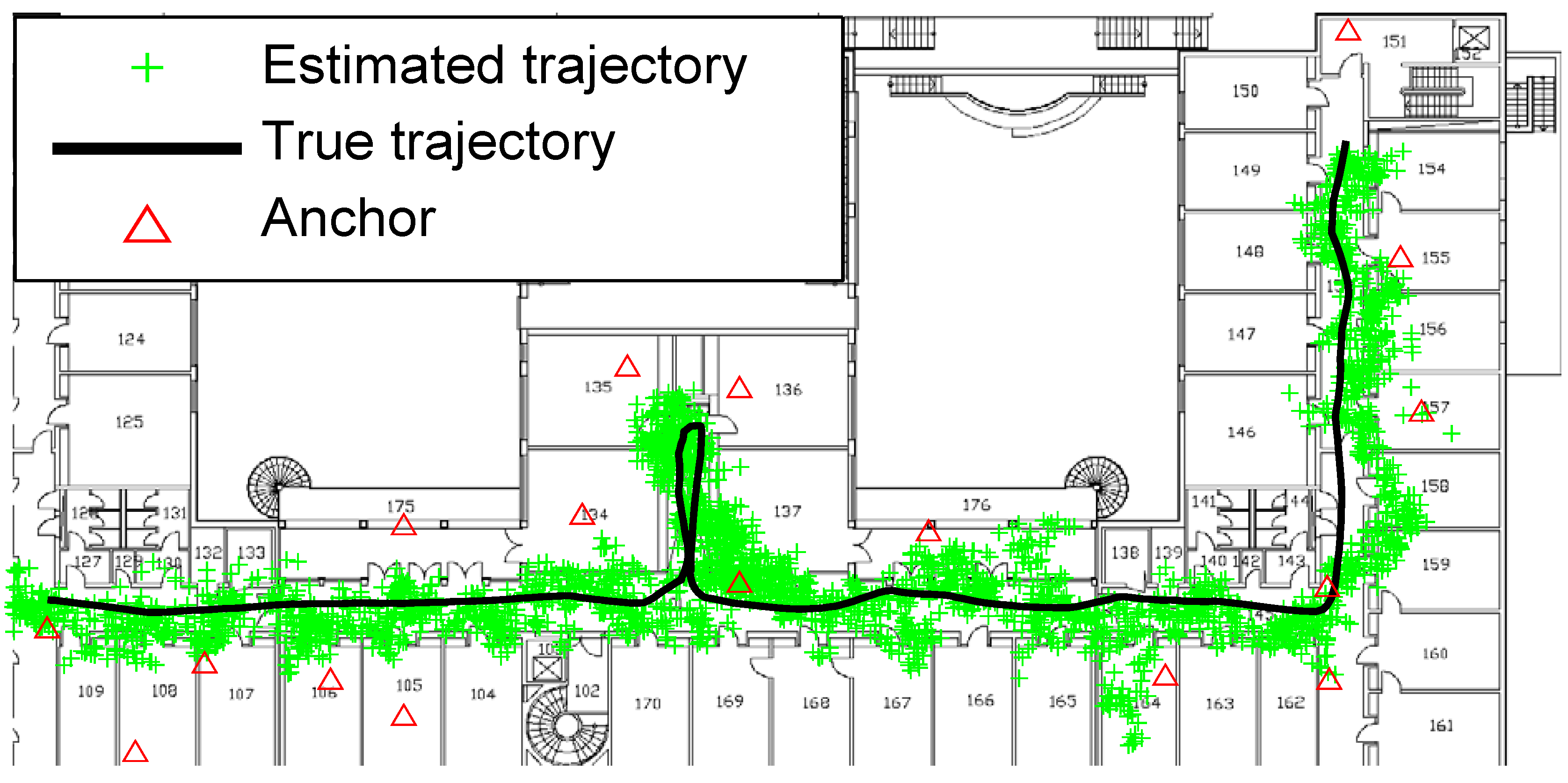
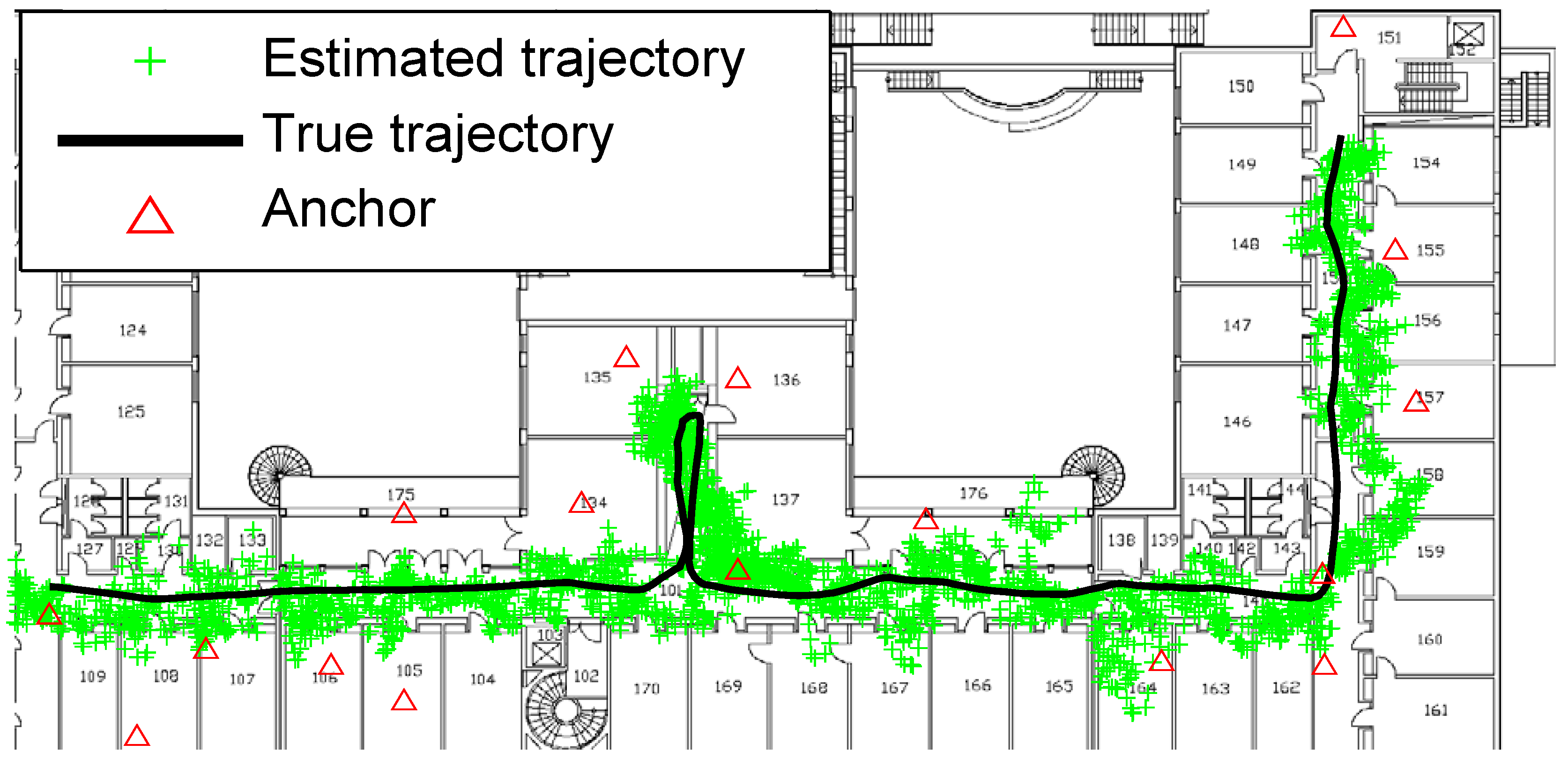
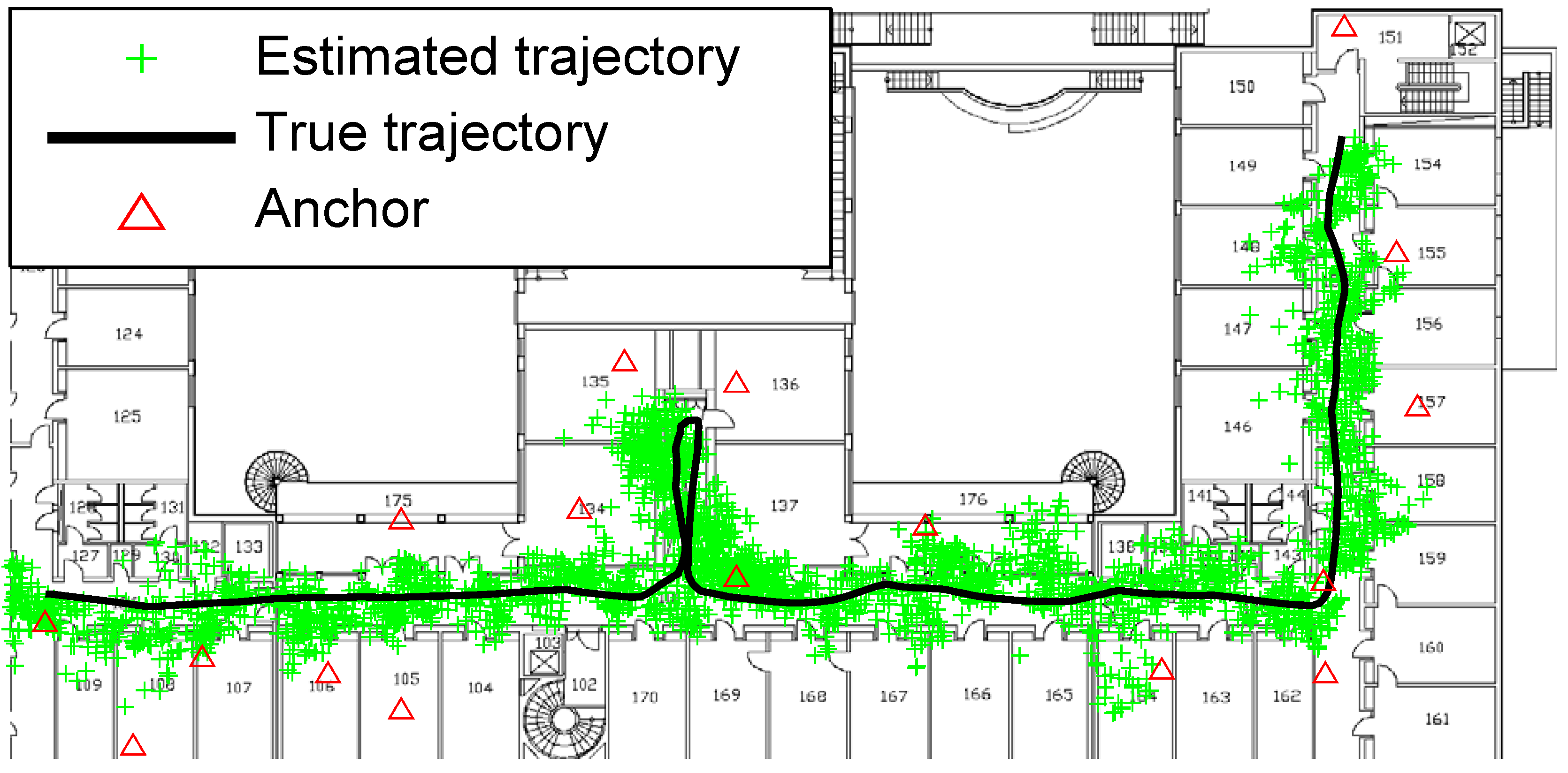
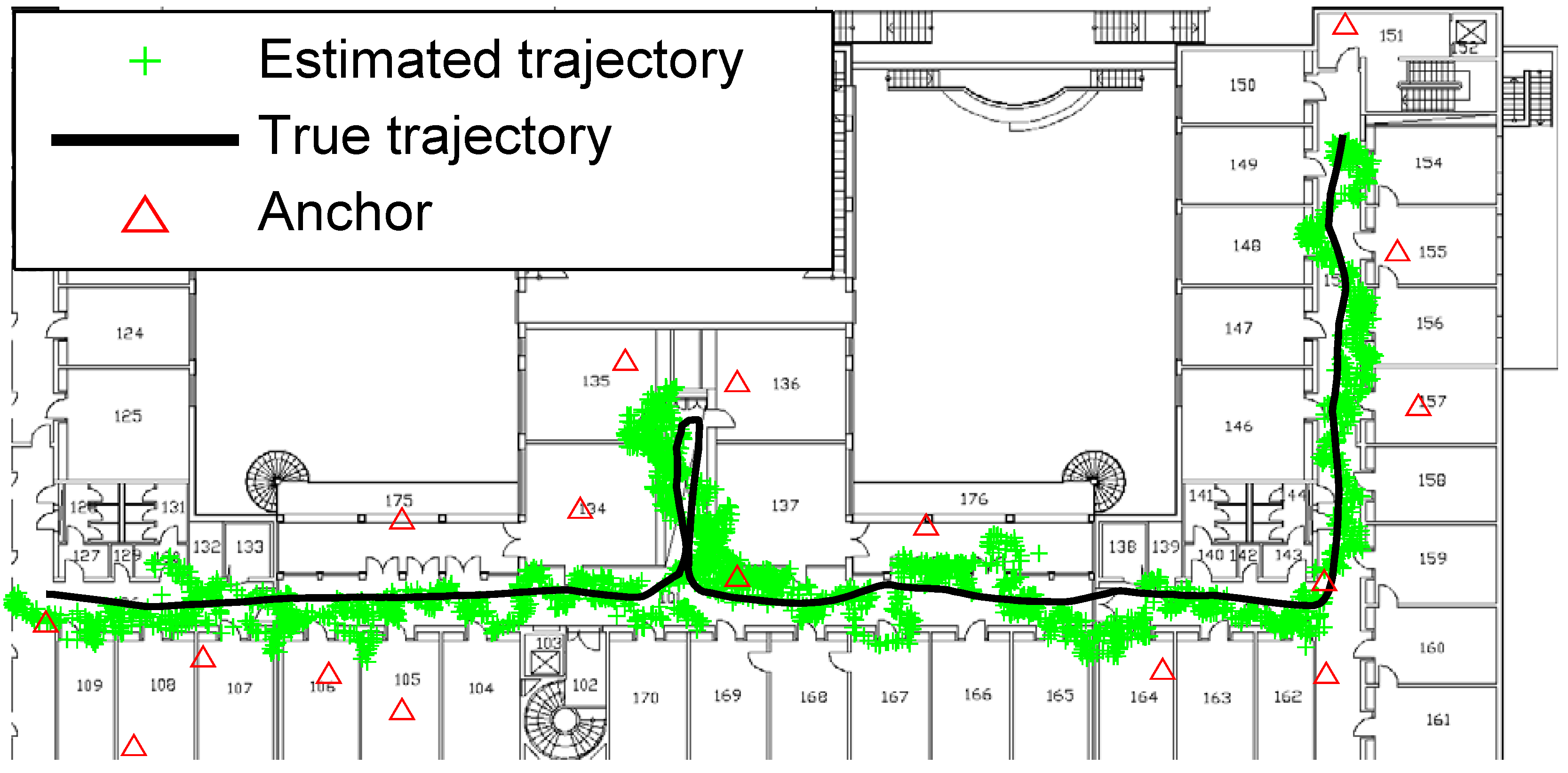
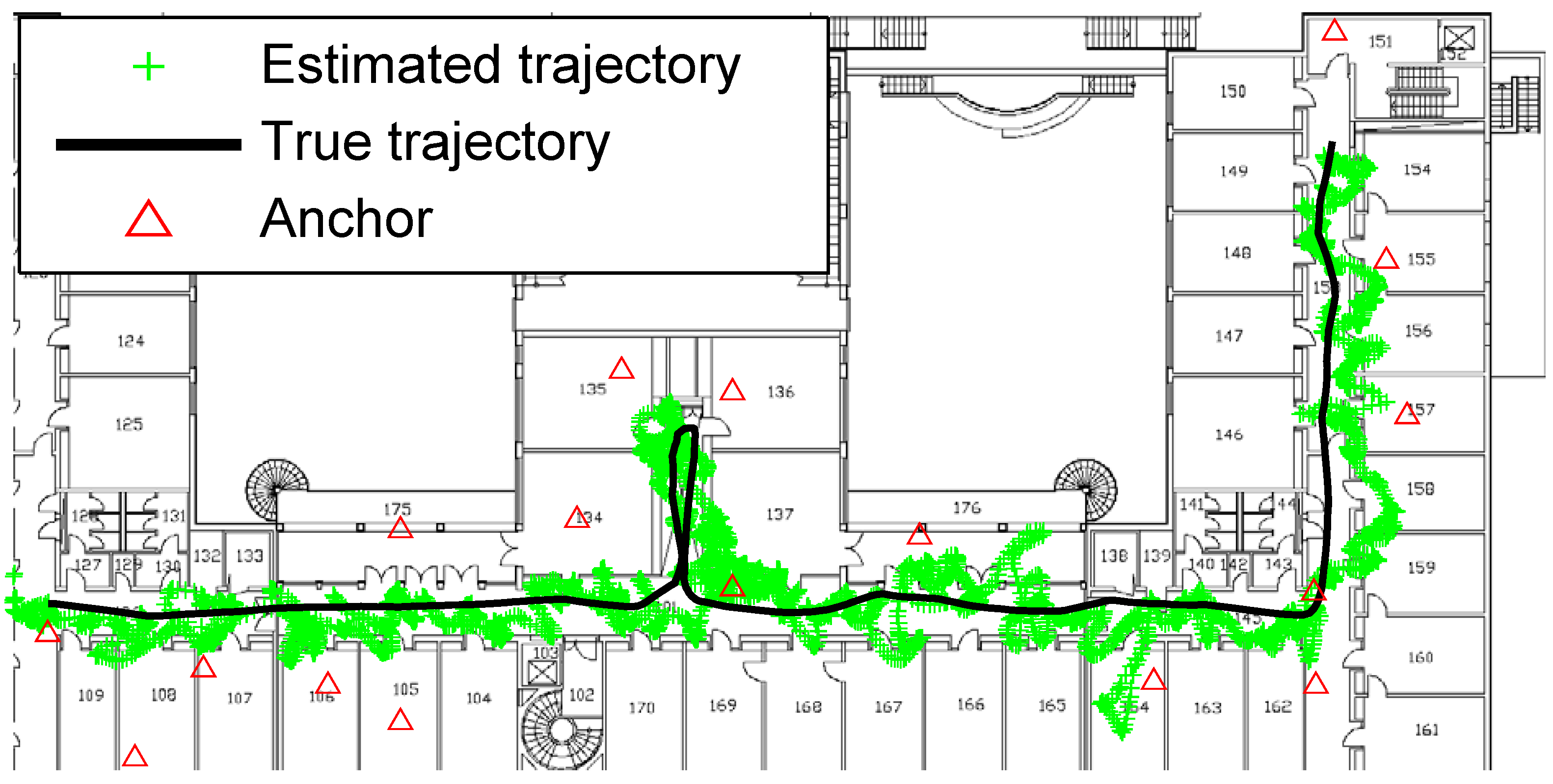
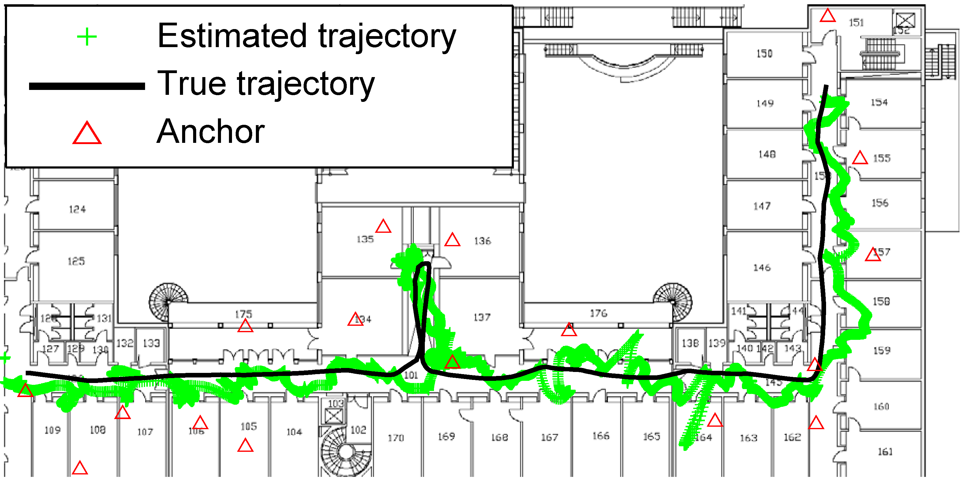
• Figure 2 shows the positioning behavior of GPF (filtering), which presents the highest deviation and divergence from the ground truth. Comparing with the smoothing methods, filtering is not qualified for indoor positioning in multipath scenarios.
• FFBS and TFS perform almost similarly to the GPF estimation (see Figure 2, Figure 3 and Figure 4), which makes a few improvements on approaching the real trajectory.
• Despite the spreading of the MPS estimation is slightly broader than that of GPF+RTS (Figure 7) and GPF+MA (Figure 6), it has a much smaller divergence to the ground truth trajectory (see Figure 5). Therefore, MPS performs the best tracking to the true trajectory, especially a better deviation and divergence when the ranging errors noise are larger (NLOS scenarios).
• The GPF+RTS (Figure 7) and GPF+MA (Figure 6) obtain much clearer estimated trajectories, as the spreading of the position estimation is much narrower; however, their estimated trajectories sometimes deviate from the true trajectory.

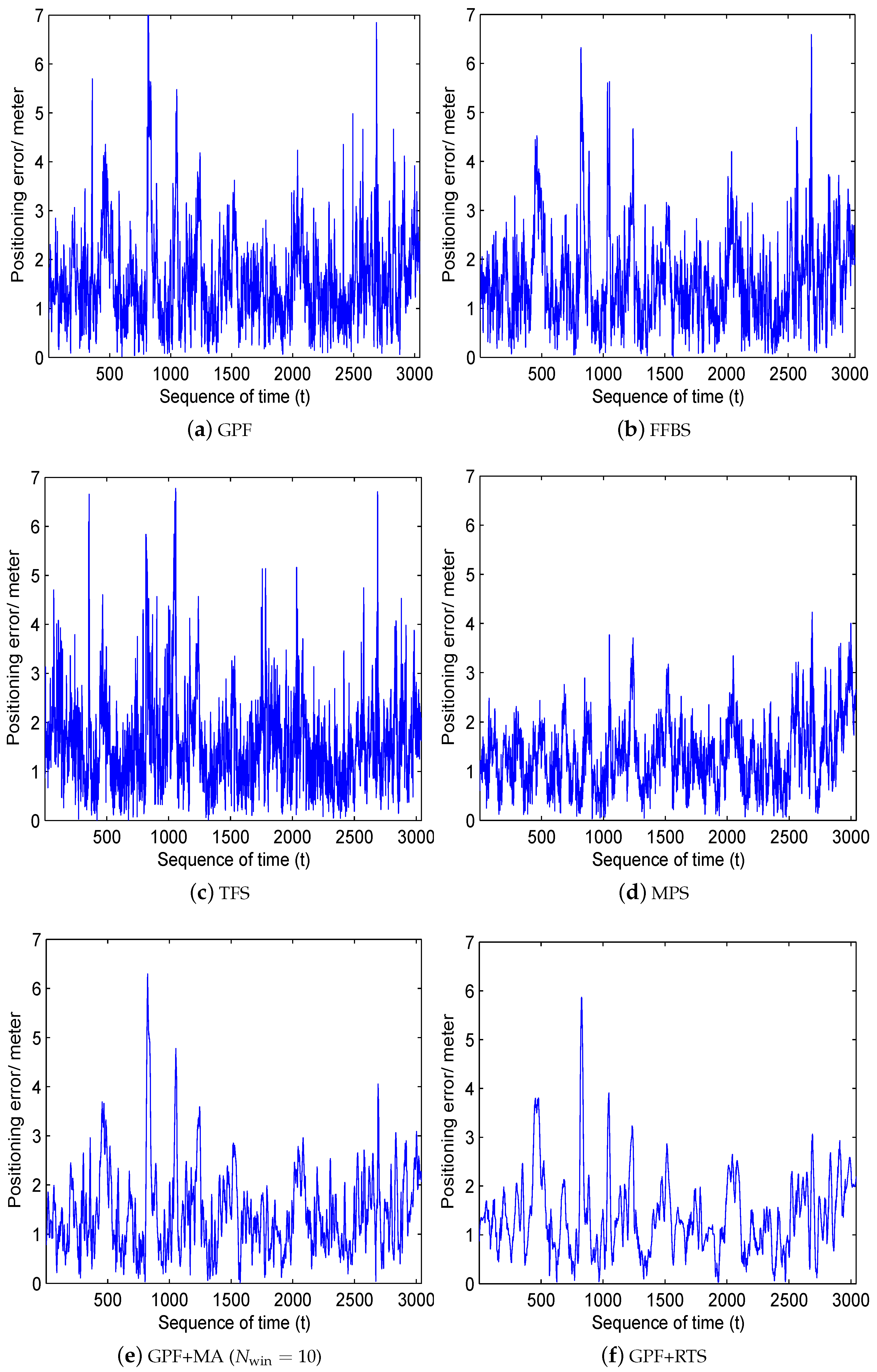
5.6. Tracking Smoothness

The smoothness of the estimated trajectory over time is depicted in Figure 8. Figure 8a displays that the estimation error of GPF fluctuates sharply indicating a higher estimation noise. The FFBS (Figure 8b) and TFS (Figure 8c) obtain almost the same instability as GPF. The MPS (Figure 8d) removes the extremely large positioning errors, whereas, it keeps the fluctuation of the small errors. The GPF+MA (Figure 8e) and GPF+RTS (Figure 8f) obviously remove the high-frequency errors, however, the very large positioning errors (the low-frequency errors) are not smoothed. Thus, the linear smoothers with a nonlinear filter are more a sense to smooth the representation of the position estimation. Over the whole moving trajectory, MPS observes the best smoothness, which removes the large positioning errors for nonlinear and non-Gaussian errors (NLOS errors). By validation in the real-world indoor tracking experiment, we summarize that

• Comparing with the filtering frame, the smoothing methods are particularly relevant for both reducing the uncertainty and smooth the representation for range-based positioning.
• The nonlinear smoothers (FFBS and TFS) are not effective, by reason that the smoothing density is not propagated into the state recursion.
• The MPS achieves much better accuracy and stability, as the smoothing density influences not only the position estimation but also the posterior recursion. In addition, its complexity is lower than the other nonlinear smoothers and remain robust against the NLOS (non-Gaussian) errors.
• The linear smoothing methods (GPF + MA and GPF + RTS) notably reduce the high-frequency fluctuation of the positioning errors, as removing the linear and Gaussian errors of the GPF estimation. However, they only work well when the smoothing lag or window size is sufficient. Moreover, they are undesirable when the target moves with a high velocity.

5.7. Discussion

Real-world indoor experiment shows that radio ranging observes a high uncertainty, which has to resort to the sequential Bayesian framework. For the nonlinear and non-Gaussian positioning problem, a closed-form Bayesian estimation is impossible to be derived. Therefore, the probabilistic estimation often explores a sample-based approximation. In the case of measurement errors and sparsity, we apply the backward smoothing to involve more information. The fundamental ingredient of applying sample-based filtering or smoothing methods to practical indoor positioning is to derive trackable density propagation. Keeping in mind that the original aim is applicable positioning, we propose to incorporate the smoothing density into the filtering density.

The results from the tracking experiment indicate that most smoothing methods can improve the tracking behavior and smooth the estimated trajectory. The proposed MPS incorporates the backward smoothing density propagation with the forward probability recursion, which is applicable for time-series estimation. Furthermore, the MPS frame can lower the time and computation complexity considerably, and mitigate the ranging errors. Comparing with prediction and filtering, MPS mitigates the nonlinear and non-Gaussian errors by taking into account more observations. Beside the smoothing frame, it is more efficient to apply a KF on the sample-based filters, which can remove the Gaussian estimation errors. Overall, These positioning algorithms achieve meter level accuracy in indoor multipath scenarios. The novelty of the proposed smoothing method is its computationally inexpensive and implementation affordable, thus, which significantly enhances the usability to other indoor scenarios.

6. Conclusions

Drawing from a smoothing density and finding an analytical solution is in most cases a difficult task, especially in case of non-linear and non-Gaussian errors. Due to the severe uncertainty of the indoor wireless environment and sensor system, range-based position tracking often encounters the LOS and NLOS measurements. To combat the uncertainty, this paper applies the Bayesian smoothing frame to the nonlinear non-Gaussian SMC models, including the FFBS, TFS, MPS, GPF + MA, and GPF + RTS. Furthermore, to be aware of the real-time constraint, we focus on the smoothing frame using a lightweight recursion.

The experiments defenestrate that the GPF+RTS and GPF+MA are more a sense to improve the representation of the estimated trajectory, whereas, the MPS filters out the estimation bias. The MPS algorithm fits the scenarios of typical motions (the mobile target with a general acceleration) and high measurement uncertainty. Since MPS requires no other assumptions, offline training, or high complexity, it is practical for its performance and efficiency. Our theoretical derivations and experimental verifications provide a better understanding of the time-series smoothing on 2D position tracking. Future work will investigate how to adaptively set the smoothing lag (the number of future observations) that achieved tradeoff of the smoothing performance and complexity. It is also useful to use the smoothing density to improve the sample quality of the SMC frame. The future work will investigate how to adaptively choose the value of the smoothing lag (the number of future observations) that leverages the tradeoff of the smoothing performance and complexity.

References

1. Liu, F.; Li, X.; Wang, J.; Zhang, J. An Adaptive UWB/MEMS-IMU Complementary Kalman Filter for Indoor Location in NLOS Environment. Remote Sens. 2019, 11, 2628. [Google Scholar] [CrossRef] [Green Version]
2. Li, X.; Deng, Z.D.; Rauchenstein, L.T.; Carlson, T.J. Contributed Review: Source-localization algorithms and applications using time of arrival and time difference of arrival measurements. Rev. Entific Instrum. 2016, 87, 921–960. [Google Scholar] [CrossRef]
3. Zhang, S.; Yu, S.; Liu, C.; Liu, S. A miniature shoe-mounted orientation determination system for accurate indoor heading and trajectory tracking. Rev. Entific Instrum. 2016, 87. [Google Scholar] [CrossRef] [PubMed]
4. Fox, V.; Hightower, J.; Liao, L.; Schulz, D.; Borriello, G. Bayesian filtering for location estimation. IEEE Pervasive Comput. 2003, 2, 24–33. [Google Scholar] [CrossRef] [Green Version]
5. Burgard, W.; Derr, A.; Fox, D.; Cremers, A.B. Integrating global position estimation and position tracking for mobile robots: The Dynamic Markov Localization approach. In Proceedings of the 1998 IEEE/RSJ International Conference on Intelligent Robots and Systems, Innovations in Theory, Practice and Applications (Cat. No. 98CH36190), Victoria, BC, Canada, 17 October 1998; Volume 2, pp. 730–735. [Google Scholar]
6. Alavi, B.; Pahlavan, K. Modeling of the TOA-based distance measurement error using UWB indoor radio measurements. IEEE Commun. Lett. 2006, 10, 275–277. [Google Scholar] [CrossRef]
7. Yu, K.; Bengtsson, M.; Ottersten, B.; McNamara, D.; Karlsson, P.; Beach, M. Modeling of wide-band MIMO radio channels based on NLoS indoor measurements. IEEE Trans. Veh. Technol. 2004, 53, 655–665. [Google Scholar] [CrossRef]
8. Yang, Y.; Zhao, Y.; Kyas, M. A non-parametric modeling of time-of-flight ranging error for indoor network localization. In Proceedings of the 2013 IEEE Global Communications Conference (GLOBECOM), Atlanta, GA, USA, 9–13 December 2013; pp. 189–194. [Google Scholar]
9. Nanopan 5375 RF Module Datasheet, Berlin, Germany. 2009. Available online: http://www.nanotron.com (accessed on 20 November 2020).
10. Lpc2738 Datasheet, Eidhoven, Neterlands. Available online: http://www.nxp.com (accessed on 20 November 2020).
11. Jennifer, H. Real-time compuall and Ogle. Transp. Res. Rec. J. Transp. Res. Board 2006, 1972, 141–150. [Google Scholar]
12. Davison, A.J. Real-time simultaneous localisation and mapping with a single camera. In Proceedings of the Ninth IEEE International Conference on Computer Vision, Nice, France, 13–16 October 2003; pp. 1403–1410. [Google Scholar]
13. Mirkin, L.; Tadmor, G. Fixed-lag smoothing as a constrained version of the fixed-interval case. In Proceedings of the IEEE 2004 American Control Conference, New York, NY, USA, 30 June–2 July 2004; Volume 5, pp. 4165–4170. [Google Scholar]
14. Kitagawa, G. Monte Carlo filter and smoother for non-Gaussian nonlinear state space models. J. Comput. Graph. Stat. 1996, 5, 1–25. [Google Scholar]
15. Yu, X.; Li, J. Optimal Filtering and a Smoothing Algorithm for a Singular System with a Complex Stochastic Uncertain Parameter Matrix. IEEE Trans. Circuits Syst. II Express Briefs 2020, 67, 780–784. [Google Scholar] [CrossRef]
16. Marchand, P.; Marmet, L. Binomial smoothing filter: A way to avoid some pitfalls of least-squares polynomial smoothing. Rev. Sci. Instrum. 1983, 54, 1034–1041. [Google Scholar] [CrossRef]
17. Xiong, Y.; Zhang, Y.; Guo, X.; Wang, C.; Shen, C.; Li, J.; Tang, J.; Liu, J. Seamless global positioning system/inertial navigation system navigation method based on square-root cubature Kalman filter and random forest regression. Rev. Sci. Instrum. 2019, 90. [Google Scholar] [CrossRef] [PubMed]
18. Feng, X.; Feng, Q.; Li, S.; Hou, X.; Liu, S. Wavelet-Based Kalman Smoothing Method for Uncertain Parameters Processing: Applications in Oil Well-Testing Data Denoising and Prediction. Sensors 2020, 20, 4541. [Google Scholar] [CrossRef] [PubMed]
19. Khalaf-Allah, M. Particle Filtering for Three-Dimensional TDoA-Based Positioning Using Four Anchor Nodes. Sensors 2020, 20, 4516. [Google Scholar] [CrossRef] [PubMed]
20. Särkkä, S. Bayesian Filtering and Smoothing; Cambridge University Press: Cambridge, UK, 2013; Volume 3. [Google Scholar]
21. Weinert, H.L. Fixed Interval Smoothing for State Space Models; Kluwer Academic Pub: Dordrecht, The Netherlands, 2001; Volume 609. [Google Scholar]
22. Doucet, A.; Johansen, A.M. A tutorial on particle filtering and smoothing: Fifteen years later. Handb. Nonlinear Filter. 2009, 12, 656–704. [Google Scholar]
23. Ait-el Fquih, B.; Desbouvries, F. Exact and approximate Bayesian smoothing algorithms in partially observed Markov chains. In Proceedings of the 2006 IEEE Nonlinear Statistical Signal Processing Workshop, Cambridge, UK, 13–15 September 2006; pp. 148–151. [Google Scholar]
24. Duong, T.T.; Chiang, K.W.; Le, D.T. On-line Smoothing and Error Modelling for Integration of GNSS and Visual Odometry. Sensors 2019, 19, 5259. [Google Scholar] [CrossRef] [PubMed] [Green Version]
25. Ito, K.; Xiong, K. Gaussian filters for nonlinear filtering problems. IEEE Trans. Autom. Control 2000, 45, 910–927. [Google Scholar] [CrossRef] [Green Version]
26. Kitagawa, G. Non-Gaussian State-Space Modeling of Nonstationary Time Series. J. Am. Stat. Assoc. 1987, 82, 1032–1041. [Google Scholar]
27. Fraser, D.; Potter, J. The optimum linear smoother as a combination of two optimum linear filters. IEEE Trans. Autom. Control 1969, 14, 387–390. [Google Scholar] [CrossRef]
28. Yang, Y.; Wu, H.; Dai, P.; Zhang, B. One Time-step Particle Smoothing for Radio Range-based Indoor Position Tracking. Electron. Lett. 2020, 56, 360–362. [Google Scholar] [CrossRef]
29. Movellan, J.; Tutorials, S.M. Discrete Time Kalman Filters and Smoothers; University of California San Diego: San Diego, CA, USA, 2011. [Google Scholar]
30. Li, X.; Wang, Y.; Khoshelham, K. Comparative analysis of robust extended Kalman filter and incremental smoothing for UWB/PDR fusion positioning in NLOS environments. Acta Geod. Geophys. 2019, 54, 157–179. [Google Scholar] [CrossRef]
31. Chen, X.; Xu, Y.; Li, Q. Application of Adaptive Extended Kalman Smoothing on INS/WSN Integration System for Mobile Robot Indoors. Math. Probl. Eng. 2013, 2013, 130508. [Google Scholar] [CrossRef]
32. Hartikainen, J.; Solin, A.; Särkkä, S. Optimal filtering with Kalman filters and smoothers. In Department of Biomedica Engineering and Computational Sciences, Aalto University School of Science, 16th August; Department of Biomedica Engineering and Computational Sciences, Aalto University School of Science: Espoo, Finland, 2011. [Google Scholar]
33. Kitagawa, G. Computational aspects of sequential Monte Carlo filter and smoother. Ann. Inst. Stat. Math. 2014, 66, 443–471. [Google Scholar] [CrossRef]
34. Lindsten, F. Rao-Blackwellised Particle Methods for Inference and Identification; Linköping University Electronic Press: Linköping, Sweden, 2011. [Google Scholar]
35. Fearnhead, P.; Wyncoll, D.; Tawn, J. A sequential smoothing algorithm with linear computational cost. Biometrika 2010, 97, 447–464. [Google Scholar] [CrossRef]
36. Hide, C.; Moore, T. GPS and low cost INS integration for positioning in the urban environment. Proc. ION GNSS 2005, 1007–1015. [Google Scholar]
37. Jun, J.; Guensler, R.; Ogle, J.H. Smoothing methods to minimize impact of Global Positioning System random error on travel distance, speed, and acceleration profile estimates. Transp. Res. Rec. J. Transp. Res. Board 2006, 1972, 141–150. [Google Scholar] [CrossRef]
38. Cao, Y.; Mao, X.C. A Nonlinear Iterative Filtering-Smoothing Algorithm for GPS Positioning. J. Shanghai Jiaotong Univ. 2009, 7, 20. [Google Scholar]
39. Liu, H.; Wang, Z.; Shan, R.; He, K.; Zhao, S. Research into the integrated navigation of a deep-sea towed vehicle with USBL/DVL and pressure gauge. Appl. Acoust. 2020, 159, 107052. [Google Scholar] [CrossRef]
40. Nurminen, H.; Ristimaki, A.; Ali-Loytty, S.; Piché, R. Particle filter and smoother for indoor localization. In Proceedings of the IEEE International Conference on Indoor Positioning and Indoor Navigation (IPIN), Montbeliard, France, 28–31 October 2013; pp. 1–10. [Google Scholar]
41. Achutegui, K.; Miguez, J.; Rodas, J.; Escudero, C.J. A multi-model sequential Monte Carlo methodology for indoor tracking: Algorithms and experimental results. Signal Process. 2012, 92, 2594–2613. [Google Scholar] [CrossRef]
42. Sukreep, S.; Nukoolkit, C.; Mongkolnam, P. Indoor Position Detection Using Smartwatch and Beacons. Sens. Mater. 2020, 32, 455–473. [Google Scholar] [CrossRef] [Green Version]
43. Radaelli, L.; Sabonis, D.; Lu, H.; Jensen, C.S. Identifying Typical Movements among Indoor Objects—Concepts and Empirical Study. In Proceedings of the IEEE International Conference on Mobile Data Management, Milan, Italy, 3–6 June 2013. [Google Scholar]
44. Hoang, M.T.; Yuen, B.; Dong, X.; Lu, T.; Westendorp, R.; Reddy Tarimala, K. Semi-Sequential Probabilistic Model for Indoor Localization Enhancement. IEEE Sens. J. 2020, 20, 6160–6169. [Google Scholar] [CrossRef] [Green Version]
45. Widyawan. Learning Data Fusion for Indoor Localisation. Ph.D. Thesis, Cork Institute of Technology, Cork, Ireland, 2009. [Google Scholar]
46. Alsindi, N.; Alavi, B.; Pahlavan, K. Measurement and modeling of ultrawideband TOA-based ranging in indoor multipath environments. IEEE Trans. Veh. Technol. 2009, 58, 1046–1058. [Google Scholar] [CrossRef]
47. Andriyanov, N.; Vasiliev, K. Using Local Objects to Improve Estimation of Mobile Object Coordinates and Smoothing Trajectory of Movement by Autoregression with Multiple Roots. Adv. Intell. Syst. Comput. 2019. [Google Scholar]
48. Kitagawa, G. The two-filter formula for smoothing and an implementation of the Gaussian-sum smoother. Ann. Inst. Stat. Math. 1994, 46, 605–623. [Google Scholar] [CrossRef]
49. Kanagal, B.; Deshpande, A. Online filtering, smoothing and probabilistic modeling of streaming data. In Proceedings of the 2008 IEEE 24th International Conference on Data Engineering, Cancun, Mexico, 7–12 April 2008; pp. 1160–1169. [Google Scholar]
50. Doucet, A.; Briers, M.; Sénécal, S. Efficient block sampling strategies for sequential Monte Carlo methods. J. Comput. Graph. Stat. 2006, 15, 693–711. [Google Scholar] [CrossRef]
51. Fearnhead, P. Sequential Monte Carlo Methods in Filter Theory. Ph.D. Thesis, University of Oxford, Oxford, UK, 1998. [Google Scholar]
52. Thrun, S.; Burgard, W.; Fox, D. Probabilistic Robotics; MIT Press: Cambridge, UK, 2005; Volume 1. [Google Scholar]
53. Briers, M.; Doucet, A.; Maskell, S. Smoothing algorithms for state–space models. Ann. Inst. Stat. Math. 2010, 62, 61–89. [Google Scholar] [CrossRef]
54. Arulampalam, M.S.; Maskell, S.; Gordon, N.; Clapp, T. A tutorial on particle filters for online nonlinear/non-Gaussian Bayesian tracking. IEEE Trans. Signal Process. 2002, 50, 174–188. [Google Scholar] [CrossRef] [Green Version]
55. Carter, C.K.; Kohn, R. On Gibbs sampling for state space models. Biometrika 1994, 81, 541–553. [Google Scholar] [CrossRef]
56. Frühwirth-Schnatter, S. Data augmentation and dynamic linear models. J. Time Ser. Anal. 1994, 15, 183–202. [Google Scholar] [CrossRef] [Green Version]
57. Creal, D. A survey of sequential Monte Carlo methods for economics and finance. Econom. Rev. 2012, 31, 245–296. [Google Scholar] [CrossRef] [Green Version]
58. Aidala, V.J. Kalman filter behavior in bearings-only tracking applications. IEEE Trans. Aerosp. Electron. Syst. 1979, 29–39. [Google Scholar] [CrossRef]
59. Haykin, S.S.; Haykin, S.S.; Haykin, S.S. Kalman Filtering and Neural Networks; Wiley Online Library: New York, NY, USA, 2001. [Google Scholar]
60. Will, H.; Hillebrandt, T.; Kyas, M. The Geo-n Localization Algorithm. In Proceedings of the IEEE International Conference on Indoor Positioning and Indoor Navigation (IPIN), Sydney, Australia, 13–15 November 2012; pp. 1–9. [Google Scholar]
61. Schmitt, S.; Will, H.; Aschenbrenner, B.; Hillebrandt, T.; Kyas, M. A reference system for indoor localization testbeds. In Proceedings of the IEEE International Conference on Indoor Positioning and Indoor Navigation (IPIN), Sydney, Australia, 13–15 November 2012; pp. 1–8. [Google Scholar]
Figure 1. Scarce LOS ranging measurements due to either the sparse anchor deployment or the NLOS scenarios: the samples circled by the red ellipse represent the condition of sparse reachable anchors; the samples surrounded by the dashed ellipse describe NLOS scenarios.
Remotesensing 12 03838 g001
Figure 2. Positioning behavior of GPF.
Remotesensing 12 03838 g002
Figure 3. Positioning behavior of FFBS.
Remotesensing 12 03838 g003
Figure 4. Positioning behavior of TFS.
Remotesensing 12 03838 g004
Figure 5. Positioning behavior of MPS.
Remotesensing 12 03838 g005
Figure 6. Positioning behavior of GPF+MA ( N win = 10 ).
Remotesensing 12 03838 g006
Figure 7. Positioning behavior of GPF+RTS.
Remotesensing 12 03838 g007
Figure 8. Positioning smoothness over time of the smoothing methods, with the sample size of SMC is N p = 49 .
Remotesensing 12 03838 g008