Visual-Inertial Odometry of Smartphone under Manhattan World

Abstract

Based on the hypothesis of the Manhattan world, we propose a tightly-coupled monocular visual-inertial odometry (VIO) system that combines structural features with point features and can run on a mobile phone in real-time. The back-end optimization is based on the sliding window method to improve computing efficiency. As the Manhattan world is abundant in the man-made environment, this regular world can use structural features to encode the orthogonality and parallelism concealed in the building to eliminate the accumulated rotation error. We define a structural feature as an orthogonal basis composed of three orthogonal vanishing points in the Manhattan world. Meanwhile, to extract structural features in real-time on the mobile phone, we propose a fast structural feature extraction method based on the known vertical dominant direction. Our experiments on the public datasets and self-collected dataset show that our system is superior to most existing open-source systems, especially in the situations where the images are texture-less, dark, and blurry.

1. Introduction

Positioning and navigation have attracted much attention in recent years, and many achievements have been made in the fields of robotics, micro aircraft, and autonomous driving. These devices can achieve very high accuracy by fusing global navigation satellite systems (GNSS), wheel-encoders, cameras, lasers, inertial measurement units (IMU), and other sensors [1,2,3]. Particularly, the fusion scheme of IMU and camera has been widely used because of its low cost and lightweight computation [4,5]. In general, the location can be obtained through GNSS outdoors, but in indoor environments, such as shopping malls and airports where GNSS is easily blocked [6,7], it becomes more difficult for people to obtain high-precision positioning services. As the smartphone is an indispensable portable device in modern life, it is particularly important to explore the potential of its positioning abilities [8]. At the same time, with the rapid development of augmented reality (AR), mobile phones have also received widespread attention as a platform for the interaction of AR technology. AR requires the mobile phone to estimate the 6 degrees of freedom (DoF) pose rather than just a 2 DoF or three DoF position [9]. The smartphone is usually equipped with at least an IMU and a consumer-level camera, which meets the minimum requirement of visual-inertial fusion.

Due to the inherent shortcomings of the temporal offsets between mobile phone sensors (camera and IMU), the motion blur generated by rolling shutter cameras [10], and the frequency reduction mechanism after overheating, etc., it is difficult to achieve a real-time estimation of the pose on mobile phones. Simultaneously, the behaviors of people when holding mobile phones are unpredictable, as they may rotate quickly for seeing the surrounding environment clearly, which may lead to blurred images. Several studies [11,12,13] that can estimate pose in real-time on mobile phones have been proposed. However, they can only eliminate the accumulated drift through loop closure, which may not exist in the paths of users. Furthermore, these methods still cannot solve the effect of image blur on rotation drift during fast rotation.

At present, the mainstreams of vision-based methods are still using point features [14,15,16], texture-less areas such as indoor corridors remain a challenge to point features-based methods. When there are few point features, the performance and accuracy of the system will be greatly degraded. Existing works use non-structural line features or structural features in the scene to deal with such difficulty. The monocular version of PL-SLAM [17] based on ORB-SLAM [15], stereo PL-SLAM [18] and PL-VIO [19] that incorporates IMU are all systems that use non-structural line features to improve the system accuracy. They match and triangulate line features between successive frames, and add line feature constraints to the residual functions by different parameterization methods.

Non-structural line features can help state estimation in the texture-less area. However, line features are unstable and easily occluded. Meanwhile, the same as point features, line features can only generate local constraints on the co-visibility graph, not a global one. By contrast, structural features can provide global observations for constraints, especially in indoor environments where most structures are man-made. The structure of this environment is usually regular and consists of three mutually orthogonal dominant directions, which is called the Manhattan world (MW) hypothesis [20]. Straight lines corresponding to each dominant direction in the space are no longer parallel in the image after projective transformation, but intersect at the vanishing point (VP) [21]. Some previous works use the structural regularity of the MW on monocular [22,23,24,25], stereo [26] and RGB-D cameras [27,28], respectively, essentially using the orthogonality of vanishing points to calculate accurate rotation or constrain the relative rotation between frames. From these works, it can be seen that the structural feature can eliminate the accumulative rotation drift of the system. Moreover, Zhou et al. [29] show that the rotation error is the main reason for long-term drift.

In our proposed method, we add the structural feature constraint to the tightly-coupled optimization-based visual-inertial odometry (VIO). We use the reprojection constraint of the point features and the global observation constraint of the structural features for state estimation. Furthermore, orthogonality between structural features is taken into account. We also optimize the process of the structural feature extraction in order to reduce the computing power of the mobile phone. As for precision, our method outperforms most of the state-of-the-art methods in the test on the public datasets. In the indoor field experiments with a mobile phone, the results show that our method achieves the best performance in terms of accuracy. The main contributions of this paper can be listed as follows:

• A fast structural feature extraction method that can run in real-time on the mobile phone is proposed. We adopt the method of exhausting VP hypotheses to obtain the optimal global solution.
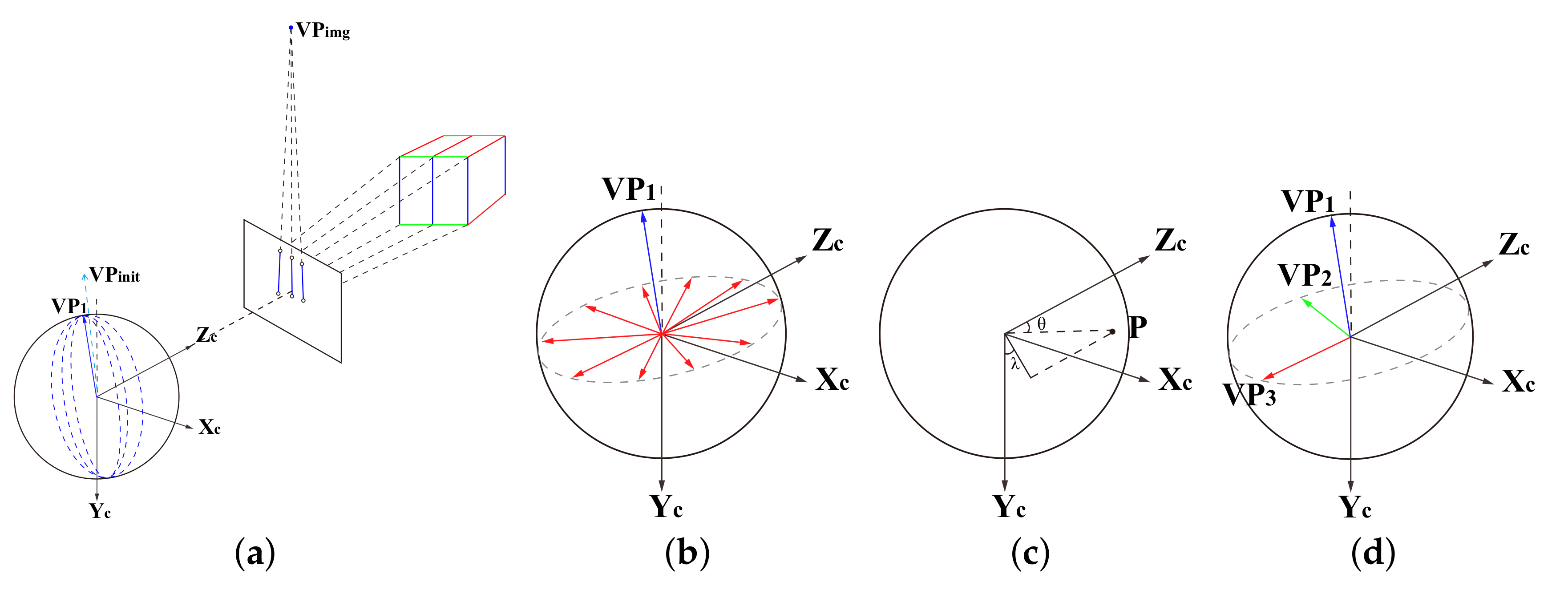
• We propose to directly parameterize the three VPs into an orthogonal basis and define the orthogonal basis as a structural feature. In mathematics, we use Hamilton quaternion to represent this orthogonal basis to avoid singularity. At the same time, we use the tangent space of the rotating manifold to update the structural feature. The orthogonality of the structural feature is considered in this updating method.
• We propose a tightly-coupled, optimization-based monocular visual-inertial odometry where IMU measurements, point features, and structural features are used as observation information. As far as we know, this is the first to add structural regularity constraint to VIO in the form of an orthogonal basis. Moreover, it can run in real-time on an Android phone with Kirin 990 5G processor at an average processing speed of 28.1 ms for a single frame.

2. Related Work

2.1. VI-SLAM and VIO

IMU provides additional observation constraints, effectively improving the robustness of the monocular vision task with motion blur and occlusion problems. Both visual-inertial simultaneous localization and mapping (VI-SLAM) and VIO can be generally divided into filtering-based methods [4,14,30] and optimization-based methods [3,16,31,32,33]. The filtering-based methods only retain the current camera state and the landmarks that may be observed in the future. Comparatively, optimization-based methods usually retain the states of multiple historical cameras and associated landmarks. The most representative filter-based methods are MSCKF [14] and ROVIO [30]. MSCKF [14] improves the algorithm efficiency by marginalizing landmarks from the state vector and reduces computation cost caused by the increase of landmarks. ROVIO [30] proposes an EKF framework that minimizes the photometric error of the patches around the point feature instead of minimizing the reprojection error.

OKVIS [32] is a classical optimization-based VIO system. It is the first to combine the optimization-based tightly-coupled method with the sliding window, and the constraints of the old states to the states in the sliding window are preserved by marginalization. The sliding window mechanism can help to maintain a constant computational cost. Similar to OKVIS [32], VINS-Mono [16] also uses the sliding window method as its back-end method. However, it proposes a fast and robust visual-inertial initialization method that estimates multiple states in the system. A 4 DoF pose graph optimization method is also adopted to eliminate the accumulated drift on x, y, z, and yaw angles. ORB-SLAM3 [33] recently released their work into the community, on the basis of the original [31]. Its VI-SLAM estimates multiple states of the system through Maximum-a-Posteriori (MAP) during visual-inertial initialization.

Several studies deploy SLAM systems on mobile phones for performing real-time estimation of the 6 DoF pose. RKSLAM [11] shows the AR effect of small range movement in the paper and proposes the use of a homography matrix to calculate inter-frame rotation for dealing with fast-rotating scenes. When the image is very blurry, and the point features cannot be matched, the homography matrix cannot be calculated. Piao et al. [12] replace the front end of ORB-SLAM with IMU pre-integration and KLT sparse optical flow tracking, making the average single-frame processing speed reach 23.2 ms on Android devices with a Qualcomm Snapdragon 805 processor. However, the performance is poor under fast rotation because the back end of ORB-SLAM is optimized based on the reprojection error under the local map, which will be interrupted during rapid rotation and fails to update the landmarks. VINS-Mobile [13] proposes a fast and robust initialization method to register the pose into the inertial frame and only optimizes the sliding window of the last few frames during the back-end optimization. However, maintaining a loop closure thread is a large overhead for a mobile phone and may occupy the computing resources of back-end optimization, causing frequency reduction after much heating. This paper disables the loop closure thread and allocates the computing resources to the back-end optimization.

2.2. Vanishing Point Extraction

The conventional process of VP extraction is first to extract the line segments in the image, and then cluster the extracted lines. Existing real-time VP extraction methods are mainly divided into two categories: One is the exhaustive method improved by Lu et al. [34]. They exhaustively list VPs hypotheses based on the orthogonality of VPs and construct a polar grid to speed up the VPs hypothesis query, finally improving the real-time performance. The other kind is based on RANSAC [22,35,36,37]. The initial vanishing point is usually estimated by defining the minimum solution set, namely two line segments. A random sampling algorithm iteratively generates the vanishing point hypothesis, and the optimal vanishing point is selected as the final solution. Tardif et al. [36] use the J-linkage algorithm to extract VPs without any prior information. Bazin et al. [37] propose a method to solve the VPs using 1-line RANSAC when the normal vector of the horizontal plane is known. Camposeco et al. [22] then accelerate the RANSAC line clustering process by getting the direction of gravity from the accelerometer in their VIO system. Though the RANSAC method is speedy, there is a problem that the optimal global solution cannot be obtained.

2.3. Structural Regularity

A line of works uses structural regularity in MW to improve the performance of pose estimation. Camposeco et al. [22] combine the VPs with VIO in the framework of EKF and parametrize the VPs into a tangent space on the unit circle for representation. However, they do not consider that the VPs should maintain orthogonality after parameterization. StructSLAM [23] does not directly use the VPs as observation constraints but takes the structural lines corresponding to VPs as the observation. The structural line is parameterized by the parametric plane in which it is located and the intersection point across the parametric plane. The work most similar to ours is the system proposed by Li et al. [24]. They add the VP constraints based on PL-SLAM [17] and use the VPs to correct the pose from the aspects of absolute rotation and relative rotation. The absolute rotation residual is the residual between the currently extracted MW axes and the global MW axes. Also, the idea of average rotation in Global SFM [38] is adopted to further optimize the absolute rotation. However, they think that VP measurements are noiseless, so they do not continue to adjust the extracted VPs. Some studies use the density distribution of surface normal vectors to improve the accuracy of rotation estimation. LPVO [27] improves a mean-shift algorithm based on the normal vectors density distribution of the surface proposed by MVO [29]. LPVO uses the RGB image to extract line segments to generate the vanishing direction hypotheses. The accuracy of rotation motion estimation is improved using the density distribution of direction vectors and surface normal vectors. Guo et al. [28] use the cost function composed of point, line, and plane features to estimate the rotation during tracing. The keyframe rotation is refined by aligning the currently extracted MW axes with the global MW axes, while Li et al. [25] conduct the surface normal prediction of the RGB image by the convolutional neural network (CNN) to replace the role of the depth camera. Such studies rely on the surface normal and are difficult to be deployed on the mobile phone, whether using an RGB-D camera or CNN. Liu et al. [26] first obtain the rotation estimation after aligning the current MW axes with the global MW axes. They then separately estimate the translation, transforming the nonlinear optimization problem into a linear optimization problem. However, they ignore the error in the initialization of the global MW axes, which would always affect the rotation estimation of the system.

3. Preliminaries

We first define the notations and coordinates used throughout the paper. We employ ${(·)}^W$ to denote the Earth’s inertial frame, ${(·)}^{B_k}$ and ${(·)}^{C_k}$ to denote the inertial frame and camera frame for the kth image. The body frame is defined to be same as the inertial frame. We use Hamilton quaternion ${}^A{\mathbf{q}}^B$ and the corresponding rotation matrix ${}^A{\mathbf{R}}^B\in \mathbf{SO}\left(3\right)$ to represent the rotation from frame $\left\{B\right\}$ to frame $\left\{A\right\}$, and $\mathbf{R}\left(\mathbf{q}\right)$ and $\mathbf{q}\left(\mathbf{R}\right)$ to represent the conversion between the quaternion and rotation matrix. ${}^A{\mathbf{p}}^B$ represents the position of frame $\left\{B\right\}$ in frame $\left\{A\right\}$. We also denote the homogeneous transformation matrix ${}^A{\mathbf{T}}^B\in \mathbf{SE}\left(3\right)$:

$$\begin{array}{c}\hfill \begin{array}{c}\hfill {}^A{\mathbf{T}}^B=\left[\begin{array}{cc}{}^A{\mathbf{R}}^B& {}^A{\mathbf{p}}^B\\ {\mathbf{0}}_{1\times 3}& \mathbf{1}\end{array}\right]{{(}^A{\mathbf{T}}^B)}^{-1}={\left[\begin{array}{cc}{{(}^A{\mathbf{R}}^B)}^T& -{(}^A{\mathbf{R}}^B{)}^T{}^A{\mathbf{p}}^B\\ {\mathbf{0}}_{1\times 3}& \mathbf{1}\end{array}\right]}_{.}\end{array}\end{array}$$

(1)

${}^B{\mathbf{q}}^C$ and ${}^B{\mathbf{p}}^C$ represent the extrinsic parameters between the inertial frame and the camera frame. Due to the temporal offset between the two sensors (IMU and camera), it is not easy to calibrate extrinsic parameters between IMU and camera in the mobile phone through open-source calibration tools such as Kalibr [39]. So we manually measure the position of the sensor mount on the printed circuit board (PCB). We employ $\widehat{(·)}$ as a noisy measurement or an estimate of the state variable. We denote that ${\left[\mathbf{q}\right]}_L$ and ${\left[\mathbf{q}\right]}_R$ are, respectively, the left and right quaternion-product matrices, moreover, ⊗ represents the multiplication operation between two quaternions [40]. Since quaternion is four-dimensional, we use the perturbation of the tangent space of the rotation manifold $\delta \theta$ in order to prevent over-parameterization, and likewise for the perturbation representation of the rotation matrix. As is illustrated in (2), where ${\left[·\right]}_{\times }$ represents the skew symmetric matrix corresponding to a vector:

$$\begin{array}{c}\hfill \begin{array}{cc}\hfill \mathbf{q}& \approx \widehat{\mathbf{q}}\otimes \left[\begin{array}{c}1\\ \frac{1}{2}\delta \theta \end{array}\right]\hfill \\ \hfill \mathbf{R}& \approx \widehat{\mathbf{R}}(\mathbf{I}+{\left[\delta \theta \right]}_{\times }).\hfill \end{array}\end{array}$$

(2)

4. Monocular Visual Inertial Odometry Based on Point and Structural Features

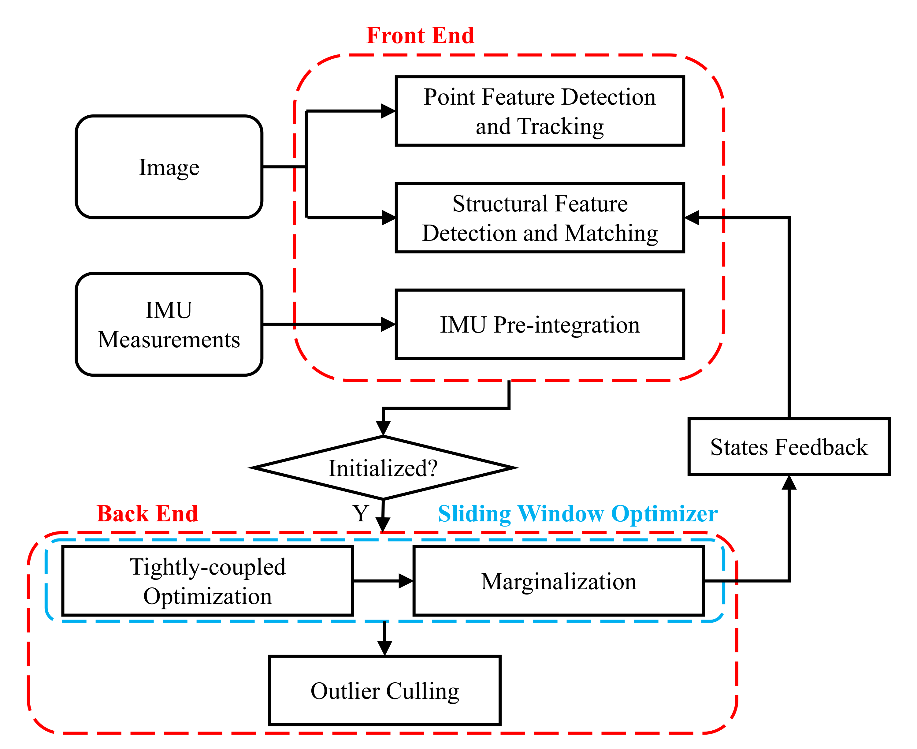
4.1. System Overview

Figure 1 shows an overview of the proposed visual-inertial odometry system. The system takes the image and IMU data flow from the mobile phone as input and outputs the estimated pose of 6 DoF. The system makes use of the rotation residuals of the structural feature on-manifold, the reprojection residuals of point feature, and the IMU pre-integration residuals for the Maximum-a-Posteriori (MAP). These observations are used as local observation constraints, while the structural features can also be used as global constraints to improve the accuracy of pose estimation. The system is mainly divided into two modules: front end and back end.

Figure 1. Pipeline of the proposed visual-inertial odometry system.

Front End. The front end receives the measurements of the image and IMU from the mobile phone, and at the same time, the old optimized states are received to match the structural features. Each time a new image comes, we update the states using IMU in the time interval of the current frame and the previous frame as the initial value for the next back-end optimization. Simultaneously, the pre-integration is used as a measurement between the continuous states during the back-end optimization, which will be described in Section 4.2.1.

The processing of acquiring point features and structural features is divided into two threads. After IMU pre-integration, we will track the old point features through the KLT sparse optical flow algorithm [41] and maintain a minimum number of point features. When the number of point features is insufficient, new point features will be added. In consideration of the efficiency, a FAST detector [42] is used to extract the corner features; furthermore, meshing and non-maximal suppression are used to control the uniform distribution of the extracted point features. We then use RANSAC with an essential model test to remove outliers. When the inlier rate is too low (lower than 0.7), we use the homograph model to perform further RANSAC verification to prevent degradation of the essential matrix due to pure rotation. While processing point features, we extract and match the structural feature of the keyframe as described in Section 4.2.2. The keyframe is decided based on the following three criteria:

• There are many newly observed landmarks.
• There are many untracked landmarks.
• The average parallax between point features matched between successive frames is large.

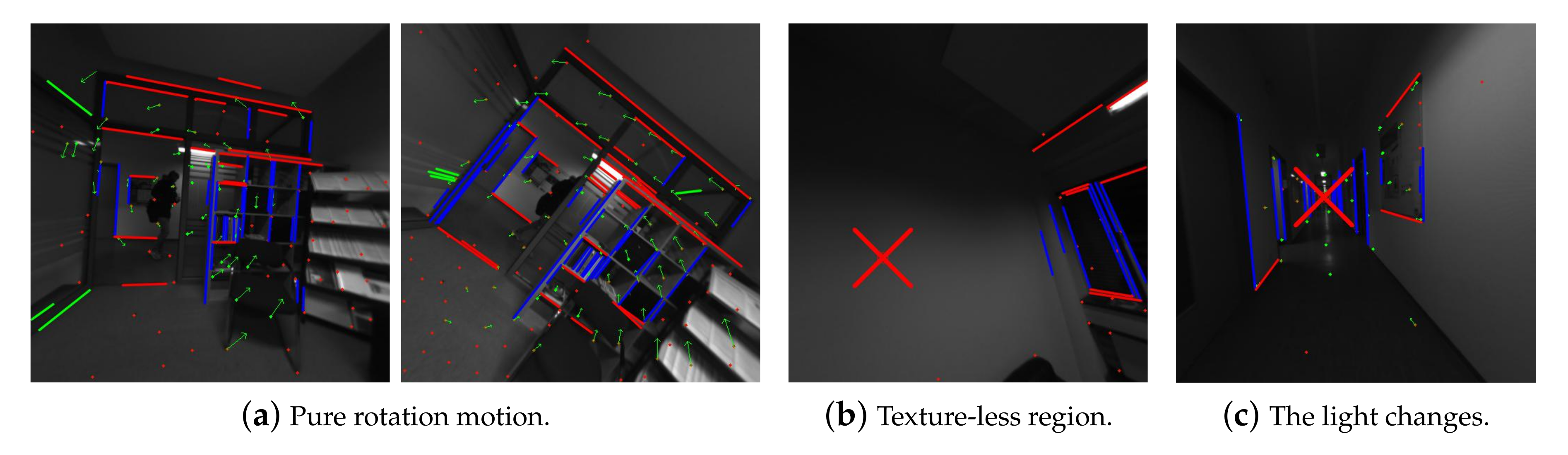
Back End. The back end is mainly based on the sliding window tightly-coupled method for state estimation. First of all, point management is carried out for the tracking results of the front-end point features. We represent landmark by the back-projection of the first observed point feature and its corresponding inverse depth. Then, according to the prior residual, point feature residuals, structural feature residuals, and IMU pre-integration residuals, a Maximum-a-Posteriori (MAP) estimation based on sliding window is carried out as described in detail in Section 4.3. Finally, landmarks and structural feature measurements with a large error need to be culled because of the change of the optimized states. If the inverse depth of the landmarks is negative, we need to cull the observations of the landmark and all corresponding point features. If the angle error between the corresponding structural feature observation of a frame in the sliding window and the maintained structural feature state is greater than the threshold (6 degrees), the corresponding structural feature observation of that frame would be culled.

4.2. Front End

4.2.1. IMU Pre-Integration

The raw measurements of the gyroscope and accelerometer can be obtained from IMU, which represents the measurements of the body frame. The gyroscope measurement ${\widehat{\mathit{\omega }}}^B$ and accelerometer measurement ${\widehat{\mathbf{a}}}^B$ are affected by gyroscope bias ${\mathbf{b}}_{\omega }^B$, accelerometer bias ${\mathbf{b}}_a^B$, gyroscope noise ${\mathbf{n}}_{\omega }^B$, and accelerometer noise ${\mathbf{n}}_a^B$. The measurements of time step t can be expressed as:

$$\begin{array}{c}\hfill \begin{array}{cc}\hfill {\widehat{\mathit{\omega }}}_t^B& ={\mathit{\omega }}_t^B+{\mathbf{b}}_{{\omega }_t}^B+{\mathbf{n}}_{{\omega }_t}^B\hfill \\ \hfill {\widehat{\mathbf{a}}}_t^B& =\mathbf{R}\left({}^{B_t}{\mathbf{q}}^W\right)({\mathbf{a}}_t^W+{\mathbf{g}}^W)+{\mathbf{b}}_{a_t}^B+{\mathbf{n}}_{a_t}^B\hfill \end{array}\end{array}$$

(3)

where $\mathbf{R}\left({}^{B_t}{\mathbf{q}}^W\right)$ rotates the acceleration of the body in the inertial frame to the representation in the body frame, and ${\mathbf{g}}^W$ is the gravity vector in the inertial frame. As in [4,16], we assume that the noises of the gyroscope and accelerometer are zero-mean Gaussian white noises, ${\mathbf{n}}_{\omega }^B\sim \mathcal{N}({\mathbf{0}}_{3\times 1},{\mathbf{\Sigma }}_{\omega })$, ${\mathbf{n}}_a^B\sim \mathcal{N}({\mathbf{0}}_{3\times 1},{\mathbf{\Sigma }}_a)$. The noises of gyroscope bias and accelerometer bias are modeled as random walk noises; therefore, its derivative are Gaussian noises, ${\mathbf{n}}_{b_{\omega }}^B\sim \mathcal{N}({\mathbf{0}}_{3\times 1},{\mathbf{\Sigma }}_{b_{\omega }})$, ${\mathbf{n}}_{b_a}^B\sim \mathcal{N}({\mathbf{0}}_{3\times 1},{\mathbf{\Sigma }}_{b_a})$.

Using the IMU measurements ${\widehat{\mathit{\omega }}}^B$ and ${\widehat{\mathbf{a}}}^B$ in the time interval of $\left[i,j\right]$, we can use (3) to propagate the body states ${}^W{\mathbf{p}}^{B_i}$, ${}^W{\mathbf{v}}^{B_i}$, ${}^W{\mathbf{q}}^{B_i}$ at time i to obtain the states ${}^W{\mathbf{p}}^{B_j}$, ${}^W{\mathbf{v}}^{B_j}$, ${}^W{\mathbf{q}}^{B_j}$ at time j. The nominal-state kinematics in continuous time is shown in (4):

$$\begin{array}{c}\hfill \begin{array}{cc}\hfill {}^W{\mathbf{p}}^{B_j}& ={}^W{\mathbf{p}}^{B_i}{+}^W{\mathbf{v}}^{B_i}\Delta t+{\int \int }_{t\in \left[i,j\right]}(\mathbf{R}\left({}^W{\mathbf{q}}^{B_t}\right)({\widehat{\mathbf{a}}}_t^B-{\mathbf{b}}_{a_t}^B)-{\mathbf{g}}^W){\delta t}^2\hfill \\ \hfill {}^W{\mathbf{v}}^{B_j}& ={}^W{\mathbf{v}}^{B_i}+{\int }_{t\in \left[i,j\right]}(\mathbf{R}({}^W{\mathbf{q}}^{B_t})({\widehat{\mathbf{a}}}_t^B-{\mathbf{b}}_{a_t}^B)-{\mathbf{g}}^W)\delta t\hfill \\ \hfill {}^W{\mathbf{q}}^{B_j}& ={\int }_{t\in \left[i,j\right]}{}^W{\mathbf{q}}^{B_t}\otimes \left[\begin{array}{c}0\\ \frac{1}{2}({\widehat{\mathit{\omega }}}^{B_t}-{\mathbf{b}}_{{\omega }_t}^B)\end{array}\right]\delta t\hfill \end{array}\end{array}$$

(4)

where $\Delta t$ is the time interval between i and j. From (4), we can see that the propagation of states is based on the position, velocity, and rotation at the time i. When the starting states change, subsequent states need to be re-propagated. Using an optimization-based approach, we need to re-propagate the IMU measurements during each iteration that will cause a change in the starting states, which is very time consuming. To avoid repeated re-propagation, we rewrite (4) as (5) and (6), and decompose the starting states from the integral, and make the integral being carried out in the local frame:

$$\begin{array}{c}\hfill \begin{array}{cc}\hfill {}^W{\mathbf{p}}^{B_j}& ={}^W{\mathbf{p}}^{B_i}{+}^W{\mathbf{v}}^{B_i}\Delta t-\frac{1}{2}{\mathbf{g}}^W{\Delta t}^2+\mathbf{R}{(}^W{\mathbf{q}}^{B_i}){}^{B_i}{\mathbf{\alpha }}^{B_j}\hfill \\ \hfill {}^W{\mathbf{v}}^{B_j}& ={}^W{\mathbf{v}}^{B_i}-{\mathbf{g}}^W\Delta t+\mathbf{R}{(}^W{\mathbf{q}}^{B_i}){}^{B_i}{\mathbf{\beta }}^{B_j}\hfill \\ \hfill {}^W{\mathbf{q}}^{B_j}& ={}^W{\mathbf{q}}^{B_i}\otimes {}^{B_i}{\mathbf{\gamma }}^{B_j}\hfill \end{array}\end{array}$$

(5)

where

$$\begin{array}{c}\hfill \begin{array}{cc}\hfill {}^{B_i}{\mathbf{\alpha }}^{B_j}& ={\int \int }_{t\in \left[i,j\right]}\mathbf{R}\left({}^{B_i}{\mathbf{q}}^{B_t}\right)({\widehat{\mathbf{a}}}_t^B-{\mathbf{b}}_{a_t}^B){\delta t}^2\hfill \\ \hfill {}^{B_i}{\mathbf{\beta }}^{B_j}& ={\int }_{t\in \left[i,j\right]}\mathbf{R}\left({}^{B_i}{\mathbf{q}}^{B_t}\right)({\widehat{\mathbf{a}}}_t^B-{\mathbf{b}}_{a_t}^B)\delta t\hfill \\ \hfill {}^{B_i}{\mathbf{\gamma }}^{B_j}& ={\int }_{t\in \left[i,j\right]}{}^{B_i}{\mathbf{q}}^{B_t}\otimes \left[\begin{array}{c}0\\ \frac{1}{2}({\widehat{\mathit{\omega }}}^{B_t}-{\mathbf{b}}_{{\omega }_t}^B)\end{array}\right]\delta t.\hfill \end{array}\end{array}$$

(6)

As can be seen from (6), the IMU integration measurements in the time interval of $\left[i,j\right]$ take $B_i$ as a reference frame, which is only related to bias and is called IMU pre-integration measurements for restricting the states of consecutive keyframes. When the bias error is slight in optimization, it will not be re-propagated, and IMU pre-integration measurement error is considered to be caused by a tiny perturbation of bias, so we use a first-order approximation to update it:

$$\begin{array}{c}\hfill \begin{array}{cc}\hfill {}^{B_i}{\mathbf{\alpha }}^{B_j}& \approx {}^{B_i}{\widehat{\mathbf{\alpha }}}^{B_j}+{\mathit{J}}_{b_{\omega }}^{\alpha }\delta {\mathbf{b}}_{{\omega }_i}^B+{\mathit{J}}_{b_a}^{\alpha }\delta {\mathbf{b}}_{a_i}^B\hfill \\ \hfill {}^{B_i}{\mathbf{\beta }}^{B_j}& \approx {}^{B_i}{\widehat{\mathbf{\beta }}}^{B_j}+{\mathit{J}}_{b_{\omega }}^{\beta }\delta {\mathbf{b}}_{{\omega }_i}^B+{\mathit{J}}_{b_a}^{\beta }\delta {\mathbf{b}}_{a_i}^B\hfill \\ \hfill {}^{B_i}{\mathbf{\gamma }}^{B_j}& \approx {}^{B_i}{\widehat{\mathbf{\gamma }}}^{B_j}\otimes \left[\begin{array}{c}1\\ \frac{1}{2}{\mathit{J}}_{b_{\omega }}^{\gamma }\delta {\mathbf{b}}_{{\omega }_i}^B\end{array}\right]\hfill \end{array}\end{array}$$

(7)

where ${\mathit{J}}_{b_{\omega }}^{\alpha },{\mathit{J}}_{b_a}^{\alpha },{\mathit{J}}_{b_{\omega }}^{\beta },{\mathit{J}}_{b_a}^{\beta },{\mathit{J}}_{b_{\omega }}^{\gamma }$ are the Jacobian matrices of IMU pre-integrated measurements with respect to bias, such as ${\mathit{J}}_{b_{\omega }}^{\alpha }=\frac{\partial {}^{B_i}{\mathbf{\alpha }}^{B_j}}{\partial \delta {\mathbf{b}}_{{\omega }_i}^B}$, which can be obtained through the error state transfer matrix.

In practice, IMU measurements need to be pre-integrated in discrete time, and sensor noises need to be considered. We propagate states at time l by mid-point integration of IMU measurements at the discrete time of l, l + 1. In (8), $\delta t_l$ is the time interval between l and l + 1:

$$\begin{array}{c}\hfill \begin{array}{cc}\hfill {}^{B_i}{\mathbf{\alpha }}^{B_{l+1}}& ={}^{B_i}{\mathbf{\alpha }}^{B_l}+{}^{B_i}{\mathbf{\beta }}^{B_l}\delta t_l+\frac{1}{2}{\overline{\mathit{a}}}^B{\delta t_l}^2\hfill \\ \hfill {}^{B_i}{\mathbf{\beta }}^{B_{l+1}}& ={}^{B_i}{\mathbf{\beta }}^{B_l}+{\overline{\mathit{a}}}^B\delta t_l\hfill \\ \hfill {}^{B_i}{\mathbf{\gamma }}^{B_{l+1}}& ={}^{B_i}{\widehat{\mathbf{\gamma }}}^{B_l}\otimes \left[\begin{array}{c}1\\ \frac{1}{2}{\overline{\mathit{\omega }}}^B\end{array}\right]\mathit{\delta }{t}_l\hfill \end{array}\end{array}$$

(8)

where

$$\begin{array}{c}\hfill \begin{array}{cc}\hfill {\overline{\mathit{a}}}^B& =\frac{1}{2}(\mathbf{R}({}^{B_i}{\mathbf{q}}^{B_l})({\widehat{\mathbf{a}}}_l^B-{\mathbf{b}}_{a_l}^B-{\mathbf{n}}_{a_l}^B)+\mathbf{R}({}^{B_i}{\mathbf{q}}^{B_{l+1}})({\widehat{\mathbf{a}}}_{l+1}^B-{\mathbf{b}}_{a_{l+1}}^B-{\mathbf{n}}_{a_{l+1}}^B))\hfill \\ \hfill {\overline{\mathit{\omega }}}^B& =\frac{1}{2}(({\widehat{\mathit{\omega }}}^{B_l}-{\mathbf{b}}_{{\omega }_l}^B-{\mathbf{n}}_{{\omega }_l}^B)+({\widehat{\mathit{\omega }}}^{B_{l+1}}-{\mathbf{b}}_{{\omega }_{l+1}}^B-{\mathbf{n}}_{{\omega }_{l+1}}^B))\hfill \end{array}\end{array}$$

(9)

Finally, as manifested in (10), we can derive the error state kinematics in discrete time based on the mid-point integration method. We represent quaternion as minimum parameterization $\mathbf{q}\approx \widehat{\mathbf{q}}\otimes \left[\begin{array}{c}1\\ \frac{1}{2}\delta \mathit{\theta }\end{array}\right]$, and we define ${\mathit{J}}_{{\theta }_l}=\mathbf{R}\left({}^{B_i}{\mathbf{q}}^{B_l}\right){\left[{\widehat{\mathbf{a}}}_l^B-{\mathbf{b}}_{a_l}^B\right]}_{\times }$.

$$\begin{array}{cc}\hfill \left[\begin{array}{c}\delta {}^{B_i}{\mathbf{\alpha }}^{B_{l+1}}\\ \delta {}^{B_i}{\mathbf{\beta }}^{B_{l+1}}\\ \delta {}^{B_i}{\mathbf{\gamma }}^{B_{l+1}}\\ \delta {\mathbf{b}}_{a_{l+1}}^B\\ \delta {\mathbf{b}}_{{\omega }_{l+1}}^B\end{array}\right]& =\left[\begin{array}{ccccc}\mathbf{I}& \mathbf{I}\delta t& -\frac{1}{4}({\mathit{J}}_{{\theta }_l}+{\mathit{J}}_{{\theta }_{l+1}}(\mathbf{I}-{\left[\mathit{\omega }\right]}_{\times }\delta t))\delta t^2& -\frac{1}{4}({}^{B_i}{\mathbf{q}}^{B_l}+{}^{B_i}{\mathbf{q}}^{B_{l+1}})\delta t^2& \frac{1}{4}{\mathit{J}}_{{\theta }_{l+1}}\delta t^3\\ \mathbf{0}& \mathbf{I}& -\frac{1}{2}({\mathit{J}}_{{\theta }_l}+{\mathit{J}}_{{\theta }_{l+1}}(\mathbf{I}-{\left[\mathit{\omega }\right]}_{\times }\delta t))\delta t& -\frac{1}{2}({}^{B_i}{\mathbf{q}}^{B_l}+{}^{B_i}{\mathbf{q}}^{B_{l+1}})\delta t& \frac{1}{2}{\mathit{J}}_{{\theta }_{l+1}}\delta t^2\\ \mathbf{0}& \mathbf{0}& \mathbf{I}-{\left[\mathit{\omega }\right]}_{\times }\delta t& \mathbf{0}& -\mathbf{I}\delta t\\ \mathbf{0}& \mathbf{0}& \mathbf{0}& \mathbf{I}& \mathbf{0}\\ \mathbf{0}& \mathbf{0}& \mathbf{0}& \mathbf{0}& \mathbf{I}\end{array}\right]\left[\begin{array}{c}\delta {}^{B_i}{\mathbf{\alpha }}^{B_l}\\ \delta {}^{B_i}{\mathbf{\beta }}^{B_l}\\ \delta {}^{B_i}{\mathbf{\gamma }}^{B_l}\\ \delta {\mathbf{b}}_{a_l}^B\\ \delta {\mathbf{b}}_{{\omega }_l}^B\end{array}\right]\hfill \\ & +\left[\begin{array}{cccccc}\frac{1}{4}{}^{B_i}{\mathbf{q}}^{B_l}\delta t^2& -\frac{1}{8}{\mathit{J}}_{{\theta }_{l+1}}\delta t^3& \frac{1}{4}{}^{B_i}{\mathbf{q}}^{B_{l+1}}\delta t^2& -\frac{1}{8}{\mathit{J}}_{{\theta }_{l+1}}\delta t^3& \mathbf{0}& \mathbf{0}\\ \frac{1}{2}{}^{B_i}{\mathbf{q}}^{B_l}\delta t& -\frac{1}{4}{\mathit{J}}_{{\theta }_{l+1}}\delta t^2& \frac{1}{2}{}^{B_i}{\mathbf{q}}^{B_{l+1}}\delta t& -\frac{1}{4}{\mathit{J}}_{{\theta }_{l+1}}\delta t^2& \mathbf{0}& \mathbf{0}\\ \mathbf{0}& \frac{1}{2}\mathbf{I}\delta t& \mathbf{0}& \frac{1}{2}\mathbf{I}\delta t& \mathbf{0}& \mathbf{0}\\ \mathbf{0}& \mathbf{0}& \mathbf{0}& \mathbf{0}& \mathbf{I}\delta t& \mathbf{0}\\ \mathbf{0}& \mathbf{0}& \mathbf{0}& \mathbf{0}& \mathbf{0}& \mathbf{I}\delta t\end{array}\right]\left[\begin{array}{c}{\mathbf{n}}_{a_l}^B\\ {\mathbf{n}}_{{\omega }_l}^B\\ {\mathbf{n}}_{a_{l+1}}^B\\ {\mathbf{n}}_{{\omega }_{l+1}}^B\\ {\mathbf{n}}_{b_a^l}^B\\ {\mathbf{n}}_{b_{\omega }^l}^B\end{array}\right]\hfill \end{array}$$

(10)

We summarize (10) and use the simplified linear model to propagate the covariance according to the forward propagation method of covariance [21]. Moreover, we can also iteratively calculate the jacobian matrix of the pre-integration measurements for the error states and provide the matrix blocks to (7).

$$\begin{array}{c}\hfill \begin{array}{cc}\hfill {\mathit{\zeta }}_{i,l+1}& =F_l{\mathit{\zeta }}_{i,l}+G_l{\mathit{n}}_{\mathbf{l}}\hfill \\ \hfill {\mathbf{\Sigma }}_{i,l+1}& =F_l{\mathbf{\Sigma }}_{i,l}{F}_l^T+G_l{\mathit{Q}}_l{G}_l^T\hfill \\ \hfill {\mathit{J}}_{i,l+1}& =F_l{\mathit{J}}_{i,l}\hfill \end{array}\end{array}$$

(11)

where ${\mathit{Q}}_l\in {\mathbb{R}}^{18\times 18}$ is the covariance matrix of the raw IMU noise and initial condition ${\mathbf{\Sigma }}_{i,i}={\mathbf{0}}_{15\times 15}$, ${\mathit{J}}_{i,i}={\mathbf{I}}_{15\times 15}$. Therefore, we can express the pre-integration noise of IMU in the time interval $\left[i,j\right]$ of two consecutive keyframes as:

$$\begin{array}{c}\hfill {\mathit{\zeta }}_{i,j}={\left[\begin{array}{ccccc}\delta {{}^{B_i}{\mathbf{\alpha }}^{B_j}}^T& \delta {{}^{B_i}{\mathbf{\beta }}^{B_j}}^T& \delta {{}^{B_i}{\mathbf{\gamma }}^{B_j}}^T& \delta {{\mathbf{b}}_{a_j}^B}^T& \delta {{\mathbf{b}}_{{\omega }_j}^B}^T\end{array}\right]}^T\sim \mathcal{N}({\mathbf{0}}_{15\times 1},{\mathbf{\Sigma }}_{i,j})\end{array}$$

(12)

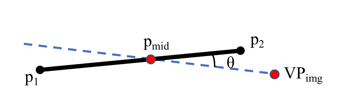
4.2.2. Structural Feature Detection and Matching

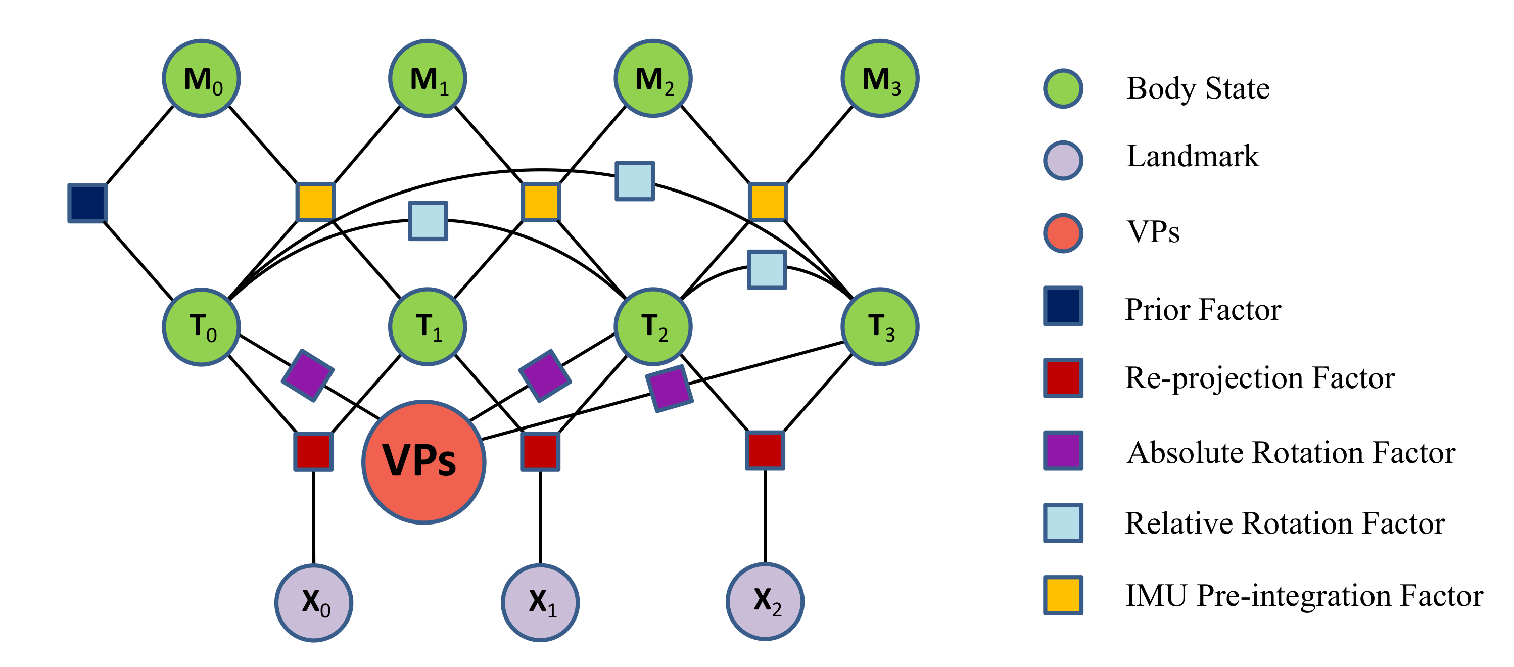
The essence of the structural feature extraction is to classify the line segments in the image and then calculate the three orthogonal dominant directions $\left\{{\mathbf{d}}_i{|}_{i=0,1,2}\right\}$. The orthogonal vanishing directions can be expressed as an orthogonal basis form, then we can obtain the representation of the structural feature in the camera frame ${}^C{\mathbf{q}}^{VPs}=\mathbf{q}\left({\left[\begin{array}{ccc}{\mathbf{d}}_0& {\mathbf{d}}_1& {\mathbf{d}}_2\end{array}\right]}_{3\times 3}\right)$. We use the EDline algorithm [43] to extract line segments. Before the initialization of the structural feature is finished, we extract VPs using a combined RANSAC and exhaustive method proposed by Lu et al. [34]. After the initialization is completed, the quick vanishing point extraction is carried out based on the known vertical direction. Suppose the angle errors between the extracted structural feature and the global state of the structural feature in each dominant direction are small (less than 6 degrees). In that case, it is considered to be a useful measurement of the structural feature.

Global state initialization for structural features

We maintain each structural feature measurement with a sliding window of the same size as the back-end sliding window. When the back-end initialization is complete, we begin the global state initialization of the structural features. Ideally, each structural feature measurement should be the same rotation ${}^W{\mathbf{q}}^{VPs}={}^W{\mathbf{q}}^B\otimes {}^B{\mathbf{q}}^C\otimes {}^C{\mathbf{q}}^{VPs}$ after being transformed to the world frame, but noise perturbation prevents them from overlapping. After the structural features in the sliding window are transformed to the world frame, spherical interpolation is carried out in turn to obtain ${}^W{\overline{\mathbf{q}}}^{VPs}$. If the angle error of each dominant direction between ${}^W{\overline{\mathbf{q}}}^{VPs}$ and the measurement of structural features in the world frame is less than the angle threshold (less than 6 degrees), the measurement is considered as an inlier. If the inlier rate is greater than 0.8, it is considered a successful initialization. Otherwise, the structural feature measurement with the maximum error is discarded.

Structural feature extraction

After the global state initialization of structural features is completed, we propose a fast and straightforward method to extract structural feature based on the known vertical direction. The whole process is shown in Figure 2.

Figure 2. These figures show the extraction process of three orthogonal VPs (structural feature). Figure (a) shows the vertical direction ${\mathbf{VP}}_{init}$ obtained after initialization is projected onto the image to obtain ${\mathbf{VP}}_{img}$, and the line segments are classified. The line segments belonging to the vertical direction are recomputed to obtain the vanishing point ${\mathbf{VP}}_1$ in the vertical direction of this frame. Figure (b) shows ${\mathbf{VP}}_2$ and ${\mathbf{VP}}_3$ hypotheses generated by uniform sampling on the circle where the normal plane of ${\mathbf{VP}}_1$ intersects the equivalent sphere. Figure (c) shows the VP hypotheses generate by all line segment pairs projected onto the polar grid. Figure (d) shows all the ${\mathbf{VP}}_2$ and ${\mathbf{VP}}_3$ hypotheses mapped into the polar grid, and the hypothesis corresponding to the maximum weight is the final global optimal VPs.

First, as shown in Figure 2a, we project the dominant vertical direction into the image to obtain ${\mathbf{VP}}_{init}$ and find the line segment set $\left\{{\mathbf{l}}_v\right\}$ belonging to this dominant direction. We define the angle between the vanishing point and the line segment, as shown in Figure 3. When the angle is less than 6 degrees, we believe that the line segment belongs to this dominant direction. We can use the $3\times n$ matrix L formed by $\left\{{\mathbf{l}}_v\right\}$ to construct the least square problem to get the first vanishing point ${\mathbf{VP}}_1$: ${\mathbf{L}}^T{\mathbf{VP}}_1={\mathbf{0}}_{n\times 1}$. It can be seen that the known vertical direction only provides us with an initial value so that we can distinguish the line segments. We consider a disturbance in ${}^W{\mathbf{q}}^C$, which leads to a slight error in the vertical direction from the world frame to the camera frame.

Figure 3. ${VP}_{img}$ is the projected position of the vanishing point in the image space, $p_1$ and $p_2$ are the two endpoints of the line segment, and $p_{mid}$ is the midpoint of the line segment. Ideally, if the segment frame is in the dominant direction corresponding to the vanishing point, then ${\mathrm{VP}}_{img}$ should be on the extension of the segment.

The orthogonal relation is satisfied between ${\mathbf{VP}}_1$ and ${\mathbf{VP}}_2$. ${\mathbf{VP}}_2$ must be on a circle formed by the intersection of the normal plane of ${\mathbf{VP}}_1$ and the equivalent sphere, as shown in Figure 2b. Therefore, we take n degree as a step size and sample uniformly on the circle to generate the hypothesis of (360/n) ${\mathbf{VP}}_{2}s$. In our work, we set n as 0.5. Meanwhile, ${\mathbf{VP}}_3$ is obtained by the cross product of ${\mathbf{VP}}_1$ and ${\mathbf{VP}}_2$.

To quickly calculate the global optimal vanishing point hypotheses, we use the polar grid proposed in [34], which maps the intersection points obtained by all line segment pairs in the image to the polar grid, and calculates the corresponding weight in Figure 2c:

$$\begin{array}{c}\hfill \begin{array}{cc}\hfill \theta & =acos({\mathbf{P}}_x/norm\left(\mathbf{P}\right))\hfill \\ \hfill \mathbf{\lambda }& =atan2({\mathbf{P}}_x,{\mathbf{P}}_y)+\pi \hfill \end{array}\end{array}$$

(13)

The weight is defined as ${\mathbf{l}}_1^{response}\times {\mathbf{l}}_2^{response}$, where the response is the proportion of the line segment in the image. This means that the vanishing point hypothesis generated by the more obvious line segment gets a higher weight. After constructing the polar grid, a gaussian smoothing filter is used to reduce the influence of measurement noise. Finally, we only need to map all ${\mathbf{VP}}_2$ and ${\mathbf{VP}}_3$ obtained from the vanishing point hypotheses into the polar grid, and select the vanishing point with the maximum corresponding weight in the polar grid as the final optimal vanishing point Figure 2d.

Structural feature matching

Our structural feature comprises three orthogonal vanishing points, so the matching problem of the structural feature is transformed into the matching problem of vanishing point direction. Since the vertical direction is known, we only have to match one dominant direction. First of all, for continuous keyframes I and J, we use ${}^W{\mathbf{q}}^{C_I}$ and ${}^W{\mathbf{q}}^{C_J}$ to convert their respective structural feature measurement to the world frame, respectively. When the included angle between dominant directions of I and J is less than 6 degrees, the structural features are considered to be well matched. In considering that if the pose drift is too large, the matching will fail. So when the above matching method fails, we use the relative rotation ${}^{C_I}{\mathbf{q}}^{C_J}$ of the IMU pre-integration between keyframes I and J to transform the structural feature measurement in I to J for rematching.

4.3. Back End

4.3.1. Tightly-Coupled Nonlinear Optimization

In this work, we first define the state variable $\mathcal{X}$ in the sliding window, which consists of body states, landmark inverse depths, and three orthogonal VPs in the Earth’s inertial frame. In our work, we define three orthogonal VPs to make up a structural feature and explain in Section 4.2.2 how to initialize the global structural feature in the inertial frame. Since VPs are calculated based on the image line segments with noises that may reflect in the global structural feature, we optimize the global structure feature as a state ${}^W{\mathbf{q}}^{VPs}$ in the sliding window. For the consistency of our VIO system, we use quaternion to represent the orthogonal basis composed of three orthogonal VPs:

$$\begin{array}{c}\hfill \begin{array}{cc}\hfill \mathcal{X}& =\left[{\left\{{\mathbf{X}}_l\right\}}_{l\in \mathcal{F}},{\left\{{\mathbf{\lambda }}_m\right\}}_{m\in \mathcal{M}},{}^W{\mathbf{q}}^{VPs}\right]\hfill \\ \hfill {\mathbf{X}}_l& =\left[{}^W{\mathbf{p}}^{B_l},{}^W{\mathbf{v}}^{B_l},{}^W{\mathbf{q}}^{B_l},{\mathbf{b}}_{a_l}^B,{\mathbf{b}}_{{\omega }_l}^B\right],l\in \mathcal{F}\hfill \end{array}\end{array}$$

(14)

where $\mathbf{X}$ is the state of the body frame corresponding to the keyframe in the sliding window, $\mathbf{\lambda }$ represents the inverse depth of each landmark, the inverse depth refers to the inverse depth corresponding to the back-projection of the starting point feature of the landmark point-track. We use $\mathcal{F}$ and $\mathcal{M}$ to denote keyframes and landmarks in the sliding window. In line with other quaternion state update strategies, we incrementally update the global structure feature state on the manifold.

Then we denote the measurement $\mathcal{Z}$ as the observation on the state $\mathcal{X}$. In (15), ${\mathbf{Z}}_l^v$ represents the point feature measurement of the mth landmark observed in the lth keyframe. If ${\mathbf{z}}_{l,m}^v$ is the starting point feature of the landmark point-track, we rewrite it as ${\mathbf{z}}_{l_s,m}^v$. ${}^{C_l}{\mathbf{q}}^{VPs}$ represents the orthogonal basis measurement of the VPs under the camera frame of the lth keyframe. ${\mathcal{B}}_{p,q}$ represents the IMU pre-integration measurements between successive keyframes p and q:

$$\begin{array}{c}\hfill \begin{array}{cc}\hfill \mathcal{Z}& =\left[{\left\{{\mathbf{Z}}_l^v,{}^{C_l}{\mathbf{q}}^{VPs}\right\}}_{l\in \mathcal{F}},{\left\{{\mathcal{B}}_{p,q}\right\}}_{(p,q)\in \mathcal{F}}\right]\hfill \\ \hfill {\mathbf{Z}}_l^v& =\left[{\left\{{\mathbf{z}}_{l,m}^v\right\}}_{m\in \mathcal{M}}\right],l\in \mathcal{F}\hfill \end{array}\end{array}$$

(15)

We apply Maximum-a-Posteriori (MAP) criterion to estimate the state of $\mathcal{X}$ with the measurement $\mathcal{Z}$, i.e.,:

$${\mathcal{X}}^{*}=\underset{\mathcal{X}}{argmax}p\left(\mathcal{X}\right|\mathcal{Z})$$

(16)

With Bayes’ rule, $\mathcal{X}|\mathcal{Z}$ in (16) can be decomposed by the prior $p\left(\mathcal{X}\right)$ and the likelihood $p\left(\mathcal{Z}\right|\mathcal{X})$, i.e.,

$$\begin{array}{c}\hfill \begin{array}{cc}\hfill p\left(\mathcal{X}\right|\mathcal{Z})\propto & p\left(\mathcal{X}\right)p\left(\mathcal{Z}\right|\mathcal{X})\hfill \\ \hfill =& p\left(\mathcal{X}\right)\prod _{(l,p,q)\in \mathcal{F}}p({\mathbf{Z}}_l^v,{}^{C_l}{\mathbf{q}}^{VPs},{\mathcal{B}}_{p,q}|\mathcal{X})\hfill \\ \hfill =& p\left(\mathcal{X}\right)\prod _{(l_s,l)\in \mathcal{F}}\prod _{m\in \mathcal{M}}p({\mathbf{z}}_{l_s,m}^v,{\mathbf{z}}_{l,m}^v|{\mathbf{X}}_{l_s},{\mathbf{X}}_l,{\mathbf{\lambda }}_m)\prod _{l\in \mathcal{F}}p\left({}^{C_l}{\mathbf{q}}^{VPs}\right|{\mathbf{X}}_l,{}^W{\mathbf{q}}^{VPs})\hfill \\ & \prod _{l_1\in \mathcal{F}}\prod _{l_2\in \mathcal{F}}p({}^{C_{l_1}}{\mathbf{q}}^{VPs},{}^{C_{l_2}}{\mathbf{q}}^{VPs}|{\mathbf{X}}_{l_1},{\mathbf{X}}_{l_2})\prod _{(p,q)\in \mathcal{F}}p\left({\mathcal{B}}_{p,q}\right|{\mathbf{X}}_p,{\mathbf{X}}_q)\hfill \end{array}\end{array}$$

(17)

Under the assumption of Gaussian distribution, we use the negative logarithm to represent the Maximum-a-Posteriori (MAP) problem, which transforms the problem into a minimum negative logarithm problem. In other words, we need to find the optimal estimation on the state $\mathcal{X}$, which can minimize the Mahalanobis norm of all measurement residuals:

$$\begin{array}{c}\hfill \begin{array}{cc}\hfill {\mathcal{X}}^{*}& =\underset{\mathcal{X}}{argmin}\{\parallel {\mathbf{r}}_P-{\mathit{H}}_P{\mathcal{X}\parallel }_{{\Sigma }_P}^2+\sum _{l\in \mathcal{F}}\sum _{m\in \mathcal{M}}\rho (\parallel {\mathbf{r}}_F({\mathbf{z}}_{l_s,m}^v,{\mathbf{z}}_{l,m}^v,\mathcal{X}){\parallel }_{{\Sigma }_F}^2)+\sum _{l\in \mathcal{F}}\rho (\parallel {\mathbf{r}}_{A_r}{(}^{C_l}{\mathbf{q}}^{VPs},\mathcal{X}){\parallel }_{{\Sigma }_{A_r}}^2)\hfill \\ & +\sum _{l_1\in \mathcal{F}}\sum _{l_2\in \mathcal{F}}\rho (\parallel {\mathbf{r}}_{R_r}({}^{C_{l_1}}{\mathbf{q}}^{VPs},{}^{C_{l_2}}{\mathbf{q}}^{VPs},\mathcal{X}){\parallel }_{{\Sigma }_{R_r}}^2)+\sum _{(p,q)\in \mathcal{F}}\parallel {\mathbf{r}}_I({\mathcal{B}}_{p,q},\mathcal{X}){\parallel }_{{\Sigma }_I}^2\}\hfill \end{array}\end{array}$$

(18)

where $\{{\mathbf{r}}_P,{\mathit{H}}_P\}$ represent the prior information obtained after the oldest keyframe is marginalized from the sliding window. ${\mathbf{r}}_F$ is the point feature of the reprojection residual. ${\mathbf{r}}_{A_r}$ is the absolute rotation residual between the structural feature measurement of keyframe and the global structural feature state. At the same time, ${\mathbf{r}}_{R_r}$ is the relative rotation residual between the structural feature measurement of each keyframe. ${\mathbf{r}}_I$ is the IMU pre-integration measurement residual between successive keyframes in the sliding window. $\rho$ is the robust function used to suppress outliers. We use the factor graph in Figure 4 to illustrate this least square problem. In this work, we use the Levenberg–Marquardt (LM) algorithm to solve this nonlinear optimization problem in (18). The detailed residual terms and Jacobian matrixes are given in the following sections.

Figure 4. The factor graph represents our optimization problem. Circles represent the states of being optimized, and squares represent the factors as probability constraints between states.

4.3.2. Point Feature Measurement Factor

We define the measurement residual of the point feature as the reprojection error on the normalized image plane. The continuous observations of the same landmark form a point-track, and there is a reprojection error between the tracked point feature and the first observation of the landmark:

$$\begin{array}{c}\hfill \begin{array}{cc}\hfill {\mathbf{r}}_F({\mathbf{z}}_{l_s,m}^v,{\mathbf{z}}_{l,m}^v,\mathcal{X})& =\left[\begin{array}{c}\frac{{\mathbf{X}}_{{\widehat{P}}_{l,m}^v}}{{\mathbf{Z}}_{{\widehat{P}}_{l,m}^v}}-{\mathbf{u}}_{P_{l,m}^v}\\ \frac{{\mathbf{Y}}_{{\widehat{P}}_{l,m}^v}}{{\mathbf{Z}}_{{\widehat{P}}_{l,m}^v}}-{\mathbf{v}}_{P_{l,m}^v}\end{array}\right]\hfill \\ \hfill {\mathbf{P}}_{l_s,m}^v& ={\pi }^{-1}({\mathbf{z}}_{l_s,m}^v,{\mathbf{\lambda }}_m)=\left[\begin{array}{c}{\mathbf{X}}_{P_{l_s,m}^v}\\ {\mathbf{Y}}_{P_{l_s,m}^v}\\ {\mathbf{Z}}_{P_{l_s,m}^v}\end{array}\right],{\mathbf{p}}_{l,m}^v={\pi }^{-1}({\mathbf{z}}_{l,m}^v)=\left[\begin{array}{c}{\mathbf{u}}_{P_{l,m}^v}\\ {\mathbf{v}}_{P_{l,m}^v}\\ \mathbf{1}\end{array}\right]\hfill \\ \hfill {\widehat{\mathbf{P}}}_{l,m}^v& ={[{({}^B{\mathbf{T}}^C)}^{-1}{\left({}^W{\mathbf{T}}^{B_l}\right)}^{-1}{}^W{\mathbf{T}}^{B_{l_s}}{}^B{\mathbf{T}}^C{\left({\mathbf{P}}_{l_s,m}^v\right)}_H]}_{0:2}\hfill \\ & ={{}^B{\mathbf{R}}^C}^T({{}^W{\mathbf{R}}^{B_l}}^T(({}^W{\mathbf{R}}^{B_{l_s}}({}^B{\mathbf{R}}^C{\mathbf{P}}_{l_s,m}^v+{}^B{\mathbf{p}}^C)+{}^W{\mathbf{p}}^{B_{l_s}})-{}^W{\mathbf{p}}^{B_l})-{}^B{\mathbf{p}}^C)\hfill \\ & =\left[\begin{array}{c}{\mathbf{X}}_{{\widehat{P}}_{l,m}^v}\\ {\mathbf{Y}}_{{\widehat{P}}_{l,m}^v}\\ {\mathbf{Z}}_{{\widehat{P}}_{l,m}^v}\end{array}\right]\hfill \end{array}\end{array}$$

(19)

${\pi }^{-1}$ is the back-projection function. According to the pixel position ${\mathbf{z}}_{l_s,m}^v$ of the landmark in the $l_s$th keyframe image when it is first observed and corresponding inverse depth ${\mathbf{\lambda }}_m$, the landmark position ${\mathbf{P}}_{l_s,m}^v$ in the $l_s$th camera frame can be obtained. H stands for the homogeneous form of the landmark position. ${\widehat{\mathbf{P}}}_{l,m}^v$ is obtained by projecting the landmark to the lth camera frame and ${\mathbf{p}}_{l,m}^v$ is the point feature measurement on the normalized image plane corresponding to the lth keyframe image. The reprojection error between ${\widehat{\mathbf{P}}}_{l,m}^v$ and ${\mathbf{p}}_{l,m}^v$ on the normalized image plane forms the point measurement residual.

We use the chain rule to derive the Jacobian matrix of the point feature factor, and the states to be optimized can be expressed as: ${\mathcal{X}}_F=\left[{}^W{\mathbf{p}}^{B_{l_s}},{}^W{\mathbf{q}}^{B_{l_s}},{}^W{\mathbf{p}}^{B_l},{}^W{\mathbf{q}}^{B_l},{\mathbf{\lambda }}_m\right]$. The Jacobian matrix is derived as follows:

$$\begin{array}{c}\hfill \begin{array}{cc}\hfill {\mathit{J}}_F& =\frac{\partial {\mathbf{r}}_F}{\partial {\widehat{\mathbf{P}}}_{l,m}^v}\left[\begin{array}{ccccc}\frac{\partial {\widehat{\mathbf{P}}}_{l,m}^v}{\partial {\mathcal{X}}_{{}^W{\mathbf{p}}^{B_{l_s}}}}& \frac{\partial {\widehat{\mathbf{P}}}_{l,m}^v}{\partial {\mathcal{X}}_{{}^W{\mathbf{q}}^{B_{l_s}}}}& \frac{\partial {\widehat{\mathbf{P}}}_{l,m}^v}{\partial {\mathcal{X}}_{{}^W{\mathbf{p}}^{B_l}}}& \frac{\partial {\widehat{\mathbf{P}}}_{l,m}^v}{\partial {\mathcal{X}}_{{}^W{\mathbf{q}}^{B_l}}}& \frac{\partial {\widehat{\mathbf{P}}}_{l,m}^v}{\partial {\mathcal{X}}_{{\mathbf{\lambda }}_m}}\end{array}\right]\hfill \\ \hfill \frac{\partial {\mathbf{r}}_F}{\partial {\widehat{\mathbf{P}}}_{l,m}^v}& =\left[\begin{array}{ccc}\frac{1}{{\mathbf{Z}}_{{\widehat{P}}_{l,m}^v}}& \mathbf{0}& -\frac{{\mathbf{X}}_{{\widehat{P}}_{l,m}^v}}{{({\mathbf{Z}}_{{\widehat{P}}_{l,m}^v})}^2}\\ \mathbf{0}& {\mathbf{Z}}_{{\widehat{P}}_{l,m}^v}& -\frac{{\mathbf{Y}}_{{\widehat{P}}_{l,m}^v}}{{({\mathbf{Z}}_{{\widehat{P}}_{l,m}^v})}^2}\end{array}\right]\hfill \\ \hfill \frac{\partial {\widehat{\mathbf{P}}}_{l,m}^v}{\partial {\mathcal{X}}_{{}^W{\mathbf{p}}^{B_{l_s}}}}& ={{}^B{\mathbf{R}}^C}^T{{}^W{\mathbf{R}}^{B_l}}^T,\frac{\partial {\widehat{\mathbf{P}}}_{l,m}^v}{\partial {\mathcal{X}}_{{}^W{\mathbf{q}}^{B_{l_s}}}}={{}^B{\mathbf{R}}^C}^T{{}^W{\mathbf{R}}^{B_l}}^T{}^W{\mathbf{R}}^{B_{l_s}}{\left[{\mathbf{P}}_{l_s,m}^{v_B}\right]}_{\times }\hfill \\ \hfill \frac{\partial {\widehat{\mathbf{P}}}_{l,m}^v}{\partial {\mathcal{X}}_{{}^W{\mathbf{p}}^{B_l}}}& =-{{}^B{\mathbf{R}}^C}^T{{}^W{\mathbf{R}}^{B_l}}^T,\frac{\partial {\widehat{\mathbf{P}}}_{l,m}^v}{\partial {\mathcal{X}}_{{}^W{\mathbf{q}}^{B_l}}}={{}^B{\mathbf{R}}^C}^T{\left[{\mathbf{P}}_{l,m}^{v_B}\right]}_{\times }\hfill \\ \hfill \frac{\partial {\widehat{\mathbf{P}}}_{l,m}^v}{\partial {\mathcal{X}}_{{\mathbf{\lambda }}_m}}& =-\frac{1}{{\mathbf{\lambda }}_m}{{}^B{\mathbf{R}}^C}^T{{}^W{\mathbf{R}}^{B_l}}^T{}^W{\mathbf{R}}^{B_{l_s}}{}^B{\mathbf{R}}^C{\mathbf{P}}_{l_s,m}^v\hfill \end{array}\end{array}$$

(20)

where

$$\begin{array}{c}\hfill \begin{array}{cc}\hfill {\mathbf{P}}_{l_s,m}^{v_B}& ={[{}^B{\mathbf{T}}^C{\left({\mathbf{P}}_{l_s,m}^v\right)}_H]}_{0:2}\hfill \\ \hfill {\mathbf{P}}_{l,m}^{v_B}& ={[{\left({}^W{\mathbf{T}}^{B_l}\right)}^{-1}{}^W{\mathbf{T}}^{B_{l_s}}{}^B{\mathbf{T}}^C{\left({\mathbf{P}}_{l_s,m}^v\right)}_H]}_{0:2}.\hfill \end{array}\end{array}$$

(21)

4.3.3. Structural Feature Measurement Factor

In order to make use of the orthogonality and parallelism of the structural feature, absolute rotation residual and relative rotation residual are defined, respectively, as the constraint factors of structure features. The absolute rotation residual is used to reduce accumulated rotation errors of our VIO system over a long time and refine the global VPs state. The relative rotation residuals are used to constrain the relative rotation between the keyframes where the structural feature can be observed.

Absolute Rotation Residual

$$\begin{array}{c}\hfill \begin{array}{cc}\hfill {\mathbf{r}}_{A_r}{(}^{C_l}{\mathbf{q}}^{VPs},\mathcal{X})& =2{[{\left({}^W{\mathbf{q}}^{VPs}\right)}^{-1}\otimes {}^W{\mathbf{q}}^{B_l}\otimes {}^B{\mathbf{q}}^C\otimes {}^{C_l}{\mathbf{q}}^{VPs}]}_{xyz}\hfill \end{array}\end{array}$$

(22)

where ${}^{C_l}{\mathbf{q}}^{VPs}$ is the measurement of the structural feature corresponding to the lth keyframe in the camera frame. ${}^W{\mathbf{q}}^{VPs}$ is a global structural feature state. The structural feature observed in this keyframe can be represented in the world frame by the body rotation ${}^W{\mathbf{q}}^{B_l}$ of this keyframe, forming an absolute rotation residual with ${}^W{\mathbf{q}}^{VPs}$.

The states to be optimized in the absolute rotation factor are ${\mathcal{X}}_{A_r}=[{}^W{\mathbf{q}}^{B_l},{}^W{\mathbf{q}}^{VPs}]$, and the corresponding Jacobian matrix is as follows:

$$\begin{array}{c}\hfill \begin{array}{cc}\hfill {\mathit{J}}_{Ar}& =\left[\begin{array}{cc}\frac{\partial {\mathbf{r}}_{Ar}}{\partial {\mathcal{X}}_{{}^W{\theta }^{B_l}}}& \frac{\partial {\mathbf{r}}_{Ar}}{\partial {\mathcal{X}}_{{}^W{\theta }^{VPs}}}\end{array}\right]\hfill \\ \hfill \frac{\partial {\mathbf{r}}_{Ar}}{\partial {\mathcal{X}}_{{}^W{\theta }^{B_l}}}& ={({[{\left({}^W{\mathbf{q}}^{VPs}\right)}^{-1}\otimes {}^W{\mathbf{q}}^{B_l}]}_L{[{}^B{\mathbf{q}}^C\otimes {}^{C_l}{\mathbf{q}}^{VPs}]}_R)}_{br}\hfill \\ \hfill \frac{\partial {\mathbf{r}}_{Ar}}{\partial {\mathcal{X}}_{{}^W{\theta }^{VPs}}}& ={({[{\left({}^W{\mathbf{q}}^{VPs}\right)}^{-1}\otimes {}^W{\mathbf{q}}^{B_l}\otimes {}^B{\mathbf{q}}^C\otimes {}^{C_l}{\mathbf{q}}^{VPs}]}_R)}_{br}\hfill \end{array}\end{array}$$

(23)

where ${(·)}_{br}$ represents the $3\times 3$ submatrix block in the bottom right corner of matrix $[·]$. Quaternion is represented by three-dimensional error state $\delta \mathit{\theta }$ to prevent over-parameterization, when updating the quaternion state, $\widehat{\mathbf{q}}\otimes \left[\begin{array}{c}1\\ \frac{1}{2}\delta \mathit{\theta }\end{array}\right]$ is used for updating.

Relative Rotation Residual

$$\begin{array}{c}\hfill \begin{array}{cc}\hfill {\mathbf{r}}_{R_r}({}^{C_{l_1}}{\mathbf{q}}^{VPs},{}^{C_{l_2}}{\mathbf{q}}^{VPs},\mathcal{X})& =2{[{({}^W{\mathbf{q}}^{B_{l_1}}\otimes {}^B{\mathbf{q}}^C\otimes {}^{C_{l_1}}{\mathbf{q}}^{VPs})}^{-1}\otimes {}^W{\mathbf{q}}^{B_{l_2}}\otimes {}^B{\mathbf{q}}^C\otimes {}^{C_{l_2}}{\mathbf{q}}^{VPs}]}_{xyz}\hfill \end{array}\end{array}$$

(24)

where ${}^{C_{l_1}}{\mathbf{q}}^{VPs}$,${}^{C_{l_2}}{\mathbf{q}}^{VPs}$ are the measurements of the structural feature corresponding to $l_1$th and $l_2$th keyframes in the camera frame, respectively. The structural feature measurement ${}^{C_{l_2}}{\mathbf{q}}^{VPs}$ in the $l_2$th keyframe can be represented in $l_1$th keyframe by the relative rotation between keyframes. Similar to the absolute rotation residual, we define the rotation error between ${}^{C_{l_2}}{\mathbf{q}}^{VPs}$ after the rotation transformation and ${}^{C_{l_1}}{\mathbf{q}}^{VPs}$ as the relative rotation residual.

For the relative rotation factor, the states associated with it to be optimized are ${\mathcal{X}}_{R_r}=[{}^W{\mathbf{q}}^{B_{l_1}},{}^W{\mathbf{q}}^{B_{l_2}}]$, and the corresponding Jacobian matrix is:

$$\begin{array}{c}\hfill \begin{array}{cc}\hfill {\mathit{J}}_{Rr}& =\left[\begin{array}{cc}\frac{\partial {\mathbf{r}}_{Rr}}{\partial {\mathcal{X}}_{{}^W{\theta }^{B_{l_1}}}}& \frac{\partial {\mathbf{r}}_{Rr}}{\partial {\mathcal{X}}_{{}^W{\theta }^{B_{l_2}}}}\end{array}\right]\hfill \\ \hfill \frac{\partial {\mathbf{r}}_{Rr}}{\partial {\mathcal{X}}_{{}^W{\theta }^{B_{l_1}}}}& =-{({[{({}^W{\mathbf{q}}^{B_{l_2}}\otimes {}^B{\mathbf{q}}^C\otimes {}^{C_{l_2}}{\mathbf{q}}^{VPs})}^{-1}\otimes {}^W{\mathbf{q}}^{B_{l_1}}]}_L{[{}^B{\mathbf{q}}^C\otimes {}^{C_{l_1}}{\mathbf{q}}^{VPs}]}_R)}_{br}\hfill \\ \hfill \frac{\partial {\mathbf{r}}_{Rr}}{\partial {\mathcal{X}}_{{}^W{\theta }^{B_{l_2}}}}& ={({[{({}^W{\mathbf{q}}^{B_{l_1}}\otimes {}^B{\mathbf{q}}^C\otimes {}^{C_{l_1}}{\mathbf{q}}^{VPs})}^{-1}\otimes {}^W{\mathbf{q}}^{B_{l_2}}]}_L{[{}^B{\mathbf{q}}^C\otimes {}^{C_{l_2}}{\mathbf{q}}^{VPs}]}_R)}_{br}\hfill \end{array}\end{array}$$

(25)

4.3.4. IMU Measurement Factor

IMU pre-integration (Section 4.2.1) can be used to constrain the states between two consecutive keyframes in the sliding window. IMU measurement residual is defined as follows:

$$\begin{array}{c}\hfill \begin{array}{c}\hfill {\mathbf{r}}_I({\mathcal{B}}_{p,q},\mathcal{X})=\left[\begin{array}{c}{\mathbf{r}}_p\\ {\mathbf{r}}_v\\ {\mathbf{r}}_{\theta }\\ {\mathbf{r}}_{b_a}\\ {\mathbf{r}}_{b_{\omega }}\end{array}\right]=\left[\begin{array}{c}{{}^W{\mathbf{R}}^{B_p}}^T({}^W{\mathbf{p}}^{B_q}-{}^W{\mathbf{p}}^{B_p}-{}^W{\mathbf{v}}^{B_p}\Delta t+\frac{1}{2}{\mathbf{g}}^W{\Delta t}^2)-{}^{B_p}{\mathbf{\alpha }}^{B_q}\\ {{}^W{\mathbf{R}}^{B_p}}^T({}^W{\mathbf{v}}^{B_q}-{}^W{\mathbf{v}}^{B_p}+{\mathbf{g}}^W\Delta t)-{}^{B_p}{\mathbf{\beta }}^{B_q}\\ 2{[{{(}^{B_p}{\mathbf{\gamma }}^{B_q})}^{-1}\otimes {\left({}^W{\mathbf{q}}^{B_p}\right)}^{-1}\otimes {}^W{\mathbf{q}}^{B_q}]}_{xyz}\\ {\mathbf{b}}_{a_q}^B-{\mathbf{b}}_{a_p}^B\\ {\mathbf{b}}_{{\omega }_q}^B-{\mathbf{b}}_{{\omega }_p}^B\end{array}\right]\end{array}\end{array}$$

(26)

where ${}^{B_p}{\mathbf{\alpha }}^{B_q}$, ${}^{B_p}{\mathbf{\beta }}^{B_q}$ and ${}^{B_p}{\mathbf{\gamma }}^{B_q}$ are the IMU pre-integration measurements, and $\Delta t$ is the time interval between the pth and qth consecutive keyframes.

IMU measurements constrain all body states of two consecutive frames, so we need to optimize ${\mathcal{X}}_I=[{\mathbf{X}}_p,{\mathbf{X}}_q]$. The Jacobian matrix corresponding to the IMU measurement residual can be obtained as:

$$\begin{array}{c}\hfill \begin{array}{cc}\hfill {\mathit{J}}_I& =\left[\begin{array}{cc}\frac{\partial {\mathbf{r}}_I}{\partial {\mathcal{X}}_{{\mathbf{X}}_p}}& \frac{\partial {\mathbf{r}}_I}{\partial {\mathcal{X}}_{{\mathbf{X}}_q}}\end{array}\right]\hfill \\ \hfill \frac{\partial {\mathbf{r}}_I}{\partial {\mathcal{X}}_{{\mathbf{X}}_p}}& ={\left[\begin{array}{ccccc}-{{}^W{\mathbf{R}}^{B_p}}^T& -{{}^W{\mathbf{R}}^{B_p}}^T\Delta t& {\left[{{}^W{\mathbf{R}}^{B_p}}^T({}^W{\mathbf{p}}^{B_q}-{}^W{\mathbf{p}}^{B_p}-{}^W{\mathbf{v}}^{B_p}\Delta t+\frac{1}{2}{\mathbf{g}}^W{\Delta t}^2)\right]}_{\times }& -{\mathit{J}}_{b_a}^{\alpha }& -{\mathit{J}}_{b_{\omega }}^{\alpha }\\ \mathbf{0}& -{{}^W{\mathbf{R}}^{B_p}}^T& {[{{}^W{\mathbf{R}}^{B_p}}^T({}^W{\mathbf{v}}^{B_q}-{}^W{\mathbf{v}}^{B_p}+{\mathbf{g}}^W\Delta t)]}_{\times }& -{\mathit{J}}_{b_a}^{\beta }& -{\mathit{J}}_{b_{\omega }}^{\beta }\\ \mathbf{0}& \mathbf{0}& {(-{[{({}^W{\mathbf{q}}^{B_q})}^{-1}\otimes {}^W{\mathbf{q}}^{B_p}]}_L{{[}^{B_p}{\mathbf{\gamma }}^{B_q}]}_R)}_{br}& \mathbf{0}& {\mathit{J}}_{b_{\omega }}^{\gamma }\\ \mathbf{0}& \mathbf{0}& \mathbf{0}& -\mathbf{I}& \mathbf{0}\\ \mathbf{0}& \mathbf{0}& \mathbf{0}& \mathbf{0}& -\mathbf{I}\end{array}\right]}_{15\times 15}\hfill \\ \hfill \frac{\partial {\mathbf{r}}_I}{\partial {\mathcal{X}}_{{\mathbf{X}}_q}}& ={\left[\begin{array}{ccccc}-{{}^W{\mathbf{R}}^{B_p}}^T& \mathbf{0}& \mathbf{0}& \mathbf{0}& \mathbf{0}\\ \mathbf{0}& {{}^W{\mathbf{R}}^{B_p}}^T& \mathbf{0}& \mathbf{0}& \mathbf{0}\\ \mathbf{0}& \mathbf{0}& {(-{[{{(}^{B_p}{\mathbf{\gamma }}^{B_q})}^{-1}\otimes {({}^W{\mathbf{q}}^{B_p})}^{-1}\otimes {}^W{\mathbf{q}}^{B_q}]}_L)}_{br}& \mathbf{0}& \mathbf{0}\\ \mathbf{0}& \mathbf{0}& \mathbf{0}& \mathbf{I}& \mathbf{0}\\ \mathbf{0}& \mathbf{0}& \mathbf{0}& \mathbf{0}& \mathbf{I}\end{array}\right]}_{15\times 15}\hfill \end{array}\end{array}$$

(27)

5. Experimental Results

We evaluate the performance of the proposed Manhattan world based VIO system on the public benchmark datasets and also in the mobile phone based indoor field tests. The state-of-the-art optimization methods are compared in both tests. We analyze the computing complexity of the proposed method, the running time of each main module is compared on the mobile phone. All of our comparative experiments are carried out on a computer with an Intel Core i5-8250 CPU at 1.6GHz, and 16 GB RAM. The Android phone we use to record the running time is HUAWEI Mate30 equipped with a Kirin 990 5G processor and 8 GB memory.

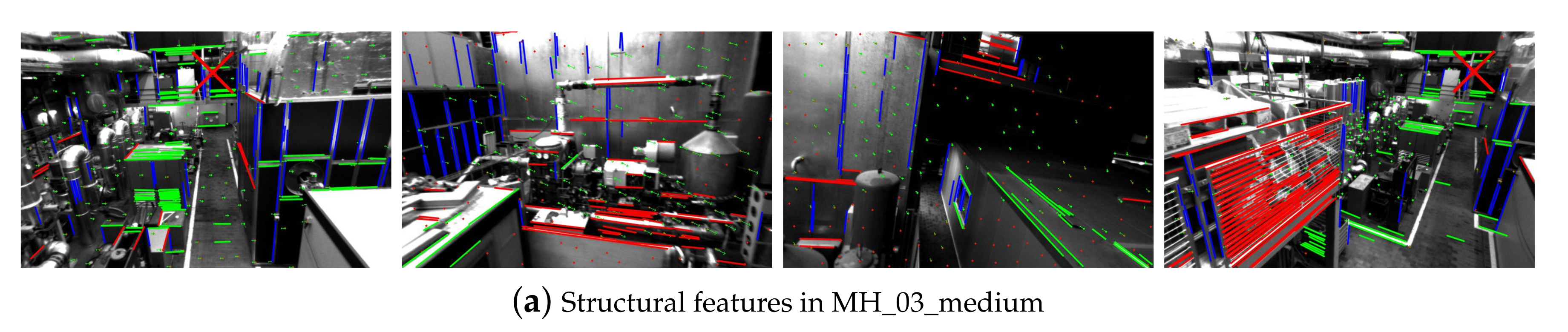
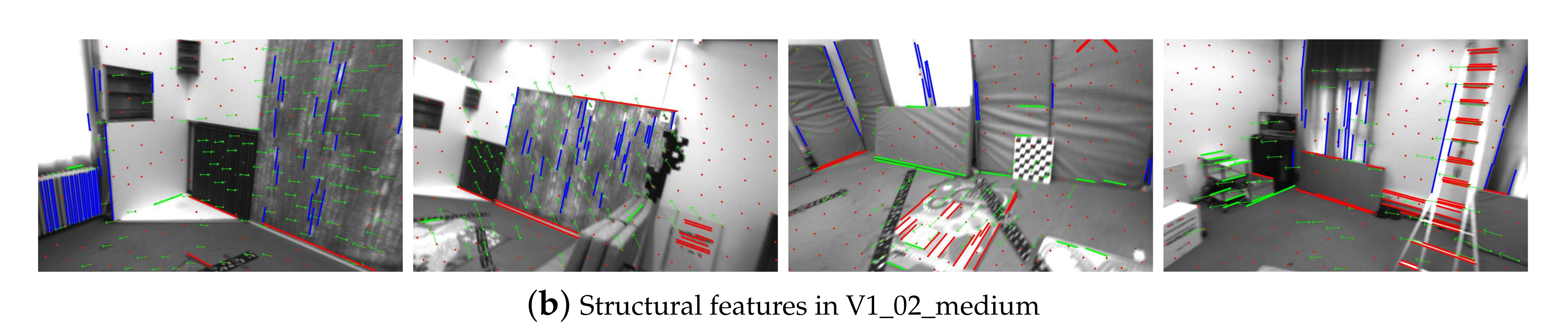
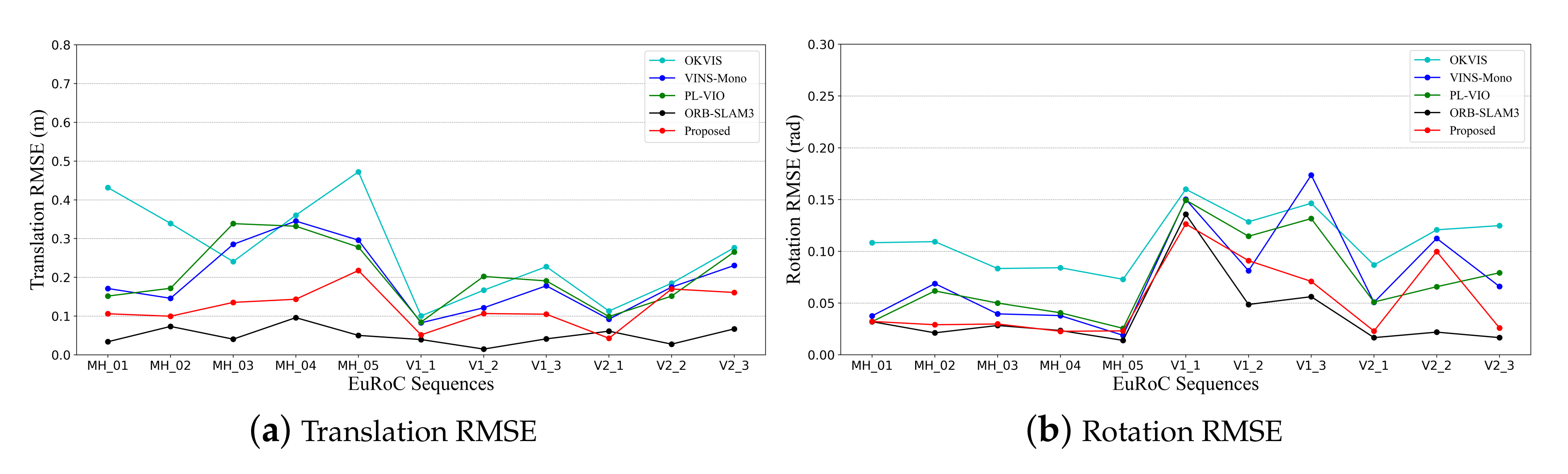
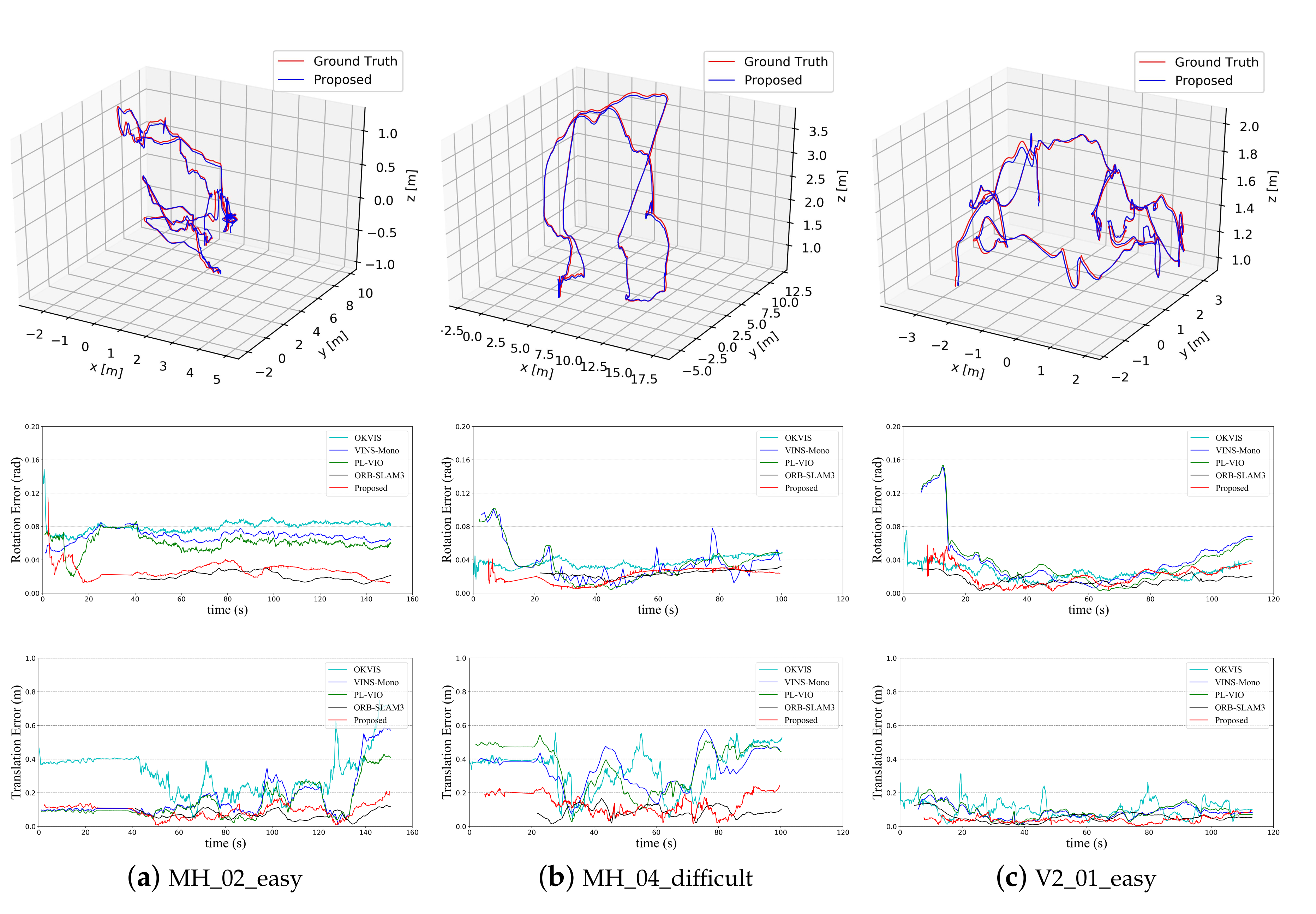
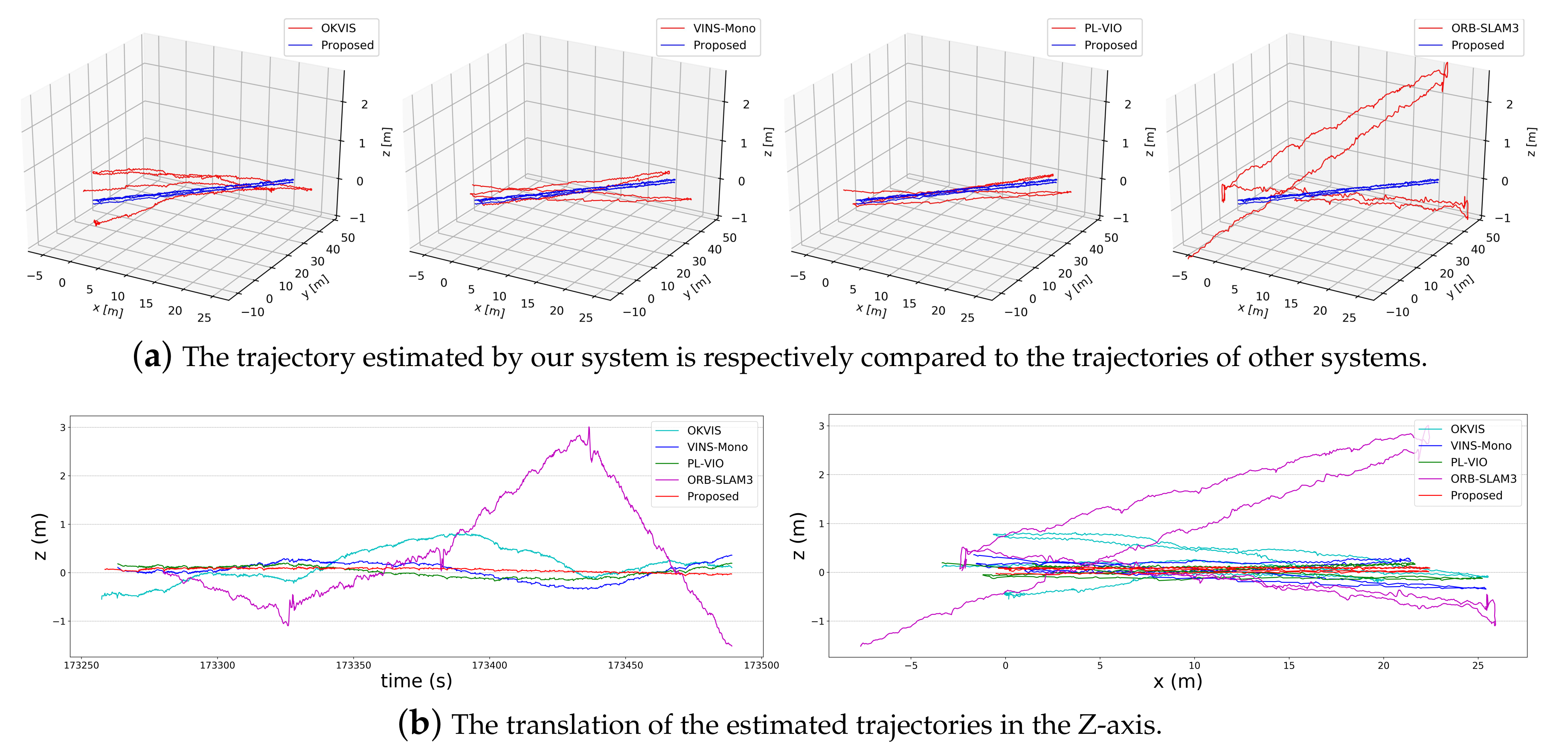
5.1. Dataset Comparison

We evaluate our VIO system on two public datasets: EuRoC dataset [44] and TUM-VI dataset [45], and we compare the performance of our system with OKVIS [32], VINS-Mono [16], PL-VIO [19], and ORB-SLAM3 [33], respectively. These are all optimization-based systems, among which OKVIS, VINS-Mono, PL-VIO are sliding window optimization-based systems, and ORB-SLAM3 is a SLAM system based on local map tracking and map reuse. OKVIS is the first VIO system to combine a sliding window approach with a tightly-coupled optimization approach. Based on the sliding window optimization, VINS-Mono adds loop closure optimization of 4 DoF and robust initialization, which results in a complete VI-SLAM system. PL-VIO adds line features based on VINS-Mono, which improves the performance of the point feature-based approach in texture-less regions. ORB-SLAM3 is a complete SLAM system containing visual, visual-inertial, and multi-map SLAM; the use of a local map for optimization can help to achieve extremely high accuracy on public datasets within centimeters.

5.1.1. EuRoC Dataset

EuRoC dataset [44] is captured by a micro aerial vehicle (MAV) in two scenes. It contains 752 × 480 resolution stereo images from global shutter cameras at 20 fps and synchronized IMU measurements at 200 Hz. The ground truth of the entire trajectory is obtained by using the VICON motion capture system. In this work, we use IMU and images from the left camera as inputs for each system.

Unlike point features and line features, structural features encode global rotation information. Regardless of the running time of the system, we can always observe the same structural feature, which can effectively reduce the accumulated rotation error of the system, as well as decrease the translation error accordingly. As shown in Figure 5, Figure 5a is processed by our system in MH_03_medium sequence, while Figure 5b is processed in V1_02_medium sequence. Red, green, and blue lines represent the three orthogonal orientations in the scene, respectively. Meanwhile, × is used to indicate the position of the vanishing point corresponding to the dominant direction of red in the image. Machine Hall in the EuRoC dataset is a scene that fully conforms to the Manhattan world hypothesis. Simultaneously, the VICON Room has some interference in other directions besides the three orthogonal directions of the room. However, our initial structural feature method can help us filter out other directions and find the three VPs corresponding to the room structure. It can be seen that the structural features are global and the MAV can observe the structural features in different places so that the accumulated errors are eliminated.

Figure 5. The performance of structural features in MH_03_medium and V1_02_medium sequences of the EuRoC dataset. The structural features encode the global rotation information and effectively restricts the accumulated rotation error, thus reducing the translation error.

The trajectories are estimated by four open-source VIO/VI-SLAM systems and our proposed system from all sequences of the EuRoC dataset. For numerical analysis, we first use $\mathbf{SE}\left(3\right)$ to align the estimated trajectory with ground truth. Absolute pose error (APE) is used as the evaluation metric of trajectory error. For the fair comparison, we use the default parameters of these open-source systems and turned off the loop closure of VINS-Mono and ORB-SLAM3. In Table 1, we give the root mean square error (RMSE) of translation and rotation between the estimated trajectories and ground truth, and corresponding line charts, as shown in Figure 6.

Table 1. The root mean square error (RMSE) of translation and rotation in all the EuRoC dataset sequences. To be easily recognized, the top 2 results of translation and rotation estimation are represented in bold fonts.

Seq.		OKVIS		VINS-Mono		PL-VIO		ORB-SLAM3		Proposed
		Trans.	Rot.	Trans.	Rot.	Trans.	Rot.	Trans.	Rot.	Trans.	Rot.
MH_01_easy		0.432	0.108	0.171	0.038	0.152	0.032	0.034${}^1$	0.032${}^1$	0.106${}^2$	0.032${}^2$
MH_02_easy		0.339	0.109	0.146	0.069	0.172	0.062	0.073${}^1$	0.021${}^1$	0.100${}^2$	0.029${}^2$
MH_03_medium		0.241	0.083	0.285	0.039	0.339	0.050	0.040${}^1$	0.028${}^1$	0.135${}^2$	0.030${}^2$
MH_04_difficult		0.360	0.084	0.345	0.038	0.332	0.041	0.096${}^1$	0.023${}^2$	0.143${}^2$	0.023${}^1$
MH_05_difficult		0.472	0.073	0.296	0.019${}^2$	0.278	0.026	0.050${}^1$	0.014${}^1$	0.218${}^2$	0.023
V1_01_easy		0.100	0.160	0.083	0.150	0.084	0.149	0.039${}^1$	0.136${}^2$	0.052${}^2$	0.126${}^1$
V1_02_medium		0.167	0.128	0.121	0.081${}^2$	0.202	0.115	0.015${}^1$	0.049${}^1$	0.107${}^2$	0.091
V1_03_difficult		0.227	0.146	0.178	0.174	0.191	0.132	0.041${}^1$	0.056${}^1$	0.105${}^2$	0.071${}^2$
V2_01_easy		0.113	0.087	0.092	0.051	0.099	0.051	0.061${}^2$	0.017${}^1$	0.043${}^1$	0.023${}^2$
V2_02_medium		0.185	0.121	0.175	0.112	0.152${}^2$	0.066${}^2$	0.028${}^1$	0.022${}^1$	0.170	0.100
V2_03_difficult		0.276	0.125	0.231	0.066	0.265	0.079	0.067${}^1$	0.017${}^1$	0.161${}^2$	0.026${}^2$

Figure 6. The comparison of root mean square error (RMSE) of translation and rotation in the EuRoC dataset.

It can be seen from Table 1 and Figure 6 that ORB-SLAM3 achieves the best performance in the EuRoC dataset, which is superior in accuracy to other systems, except for V2_01_easy sequence. The reason is that it utilizes a local map for reprojection residual constraint, which can maximize the use of historical information without loop closure. This strategy generates high map consistency when tracking point features stably. However, in addition to point feature extraction, ORB-SLAM3 also needs to calculate point feature descriptors. The point feature matching in local map tracking is $\mathit{O}\left(n^2\right)$, which presents a challenge to pose estimation on mobile phones in real-time.

Compared with the methods based on sliding window optimization such as OKVIS, VINS-Mono, and PL-VIO, we significantly improved the trajectory accuracy by utilizing the structural features. Except for MH_05_difficult, V1_02_medium, and V2_02_medium, the translation error and rotation error of other sequences are all lower than the existing similar systems. At the beginning of the V2_02_medium sequence, MAV is in a scene with a lot of outlier structure interferences, making it difficult to initialize structural features and form global constraints for an extended period. This is the main reason why the trajectory error of the proposed system in this sequence increases significantly.

We also compare the trajectory errors versus time of several sequences to show the advantages of our proposed system with structural features. Figure 7a–c represents the performance of our system in the three sequences of MH_02_easy, MH_04_difficult, and V2_01_easy, respectively. From top to bottom are the estimated trajectory, the rotation error versus time, and the translation error versus time, respectively. The rotation error of our proposed system is much smaller than that of other optimization-based methods throughout the trajectory, especially in the MH_02_easy sequence where the MAV moves stably, without too much fast motion and rotation.

Figure 7. The comparison of the trajectories of our proposed system with the ground truth and the comparison of rotation and the translation errors among all systems.

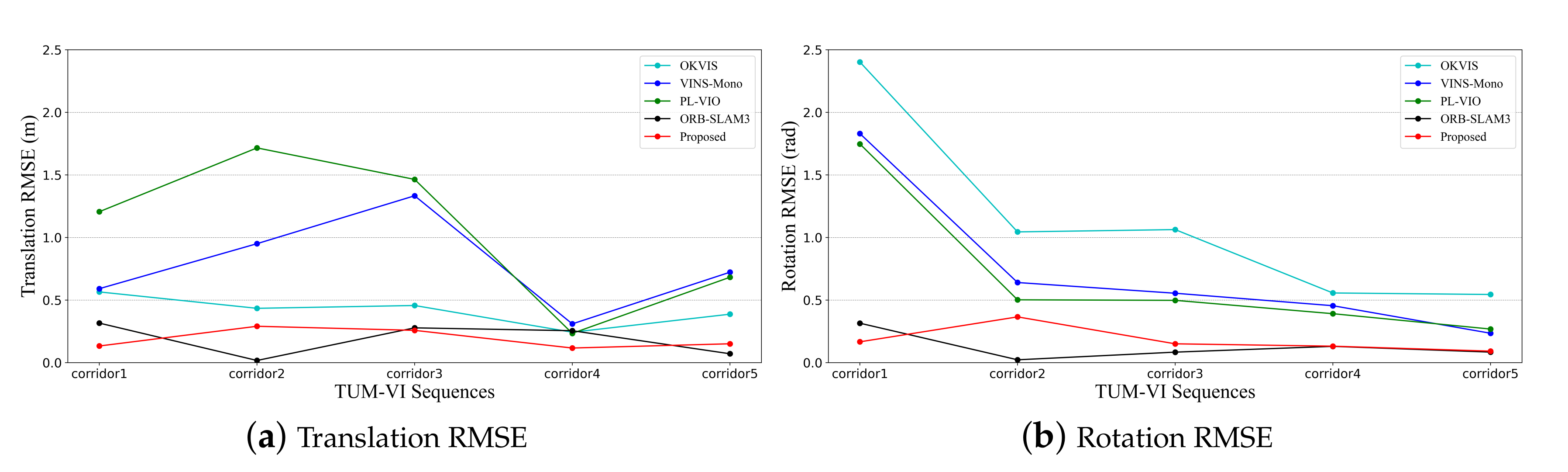
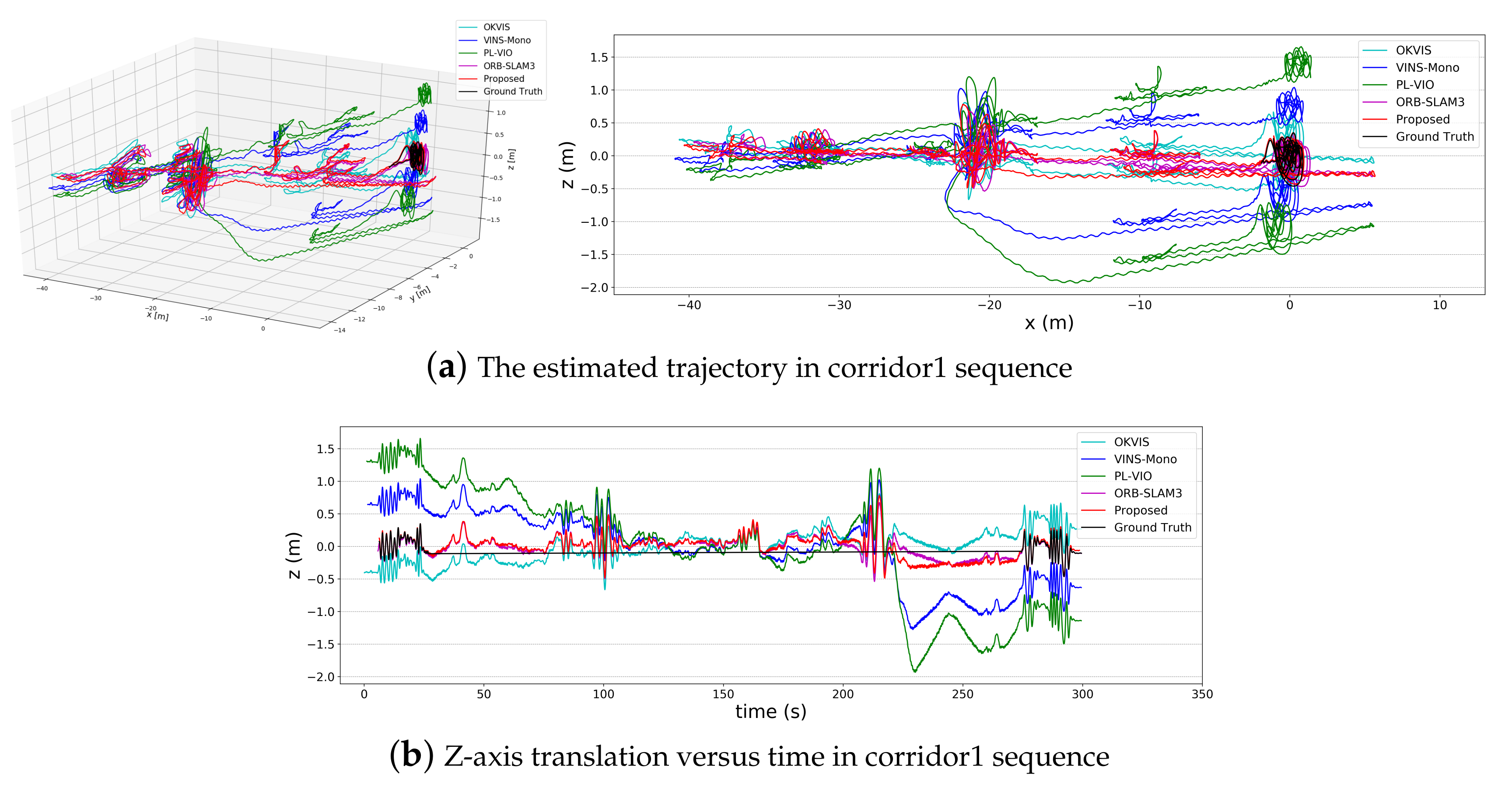
5.1.2. TUM-VI Dataset

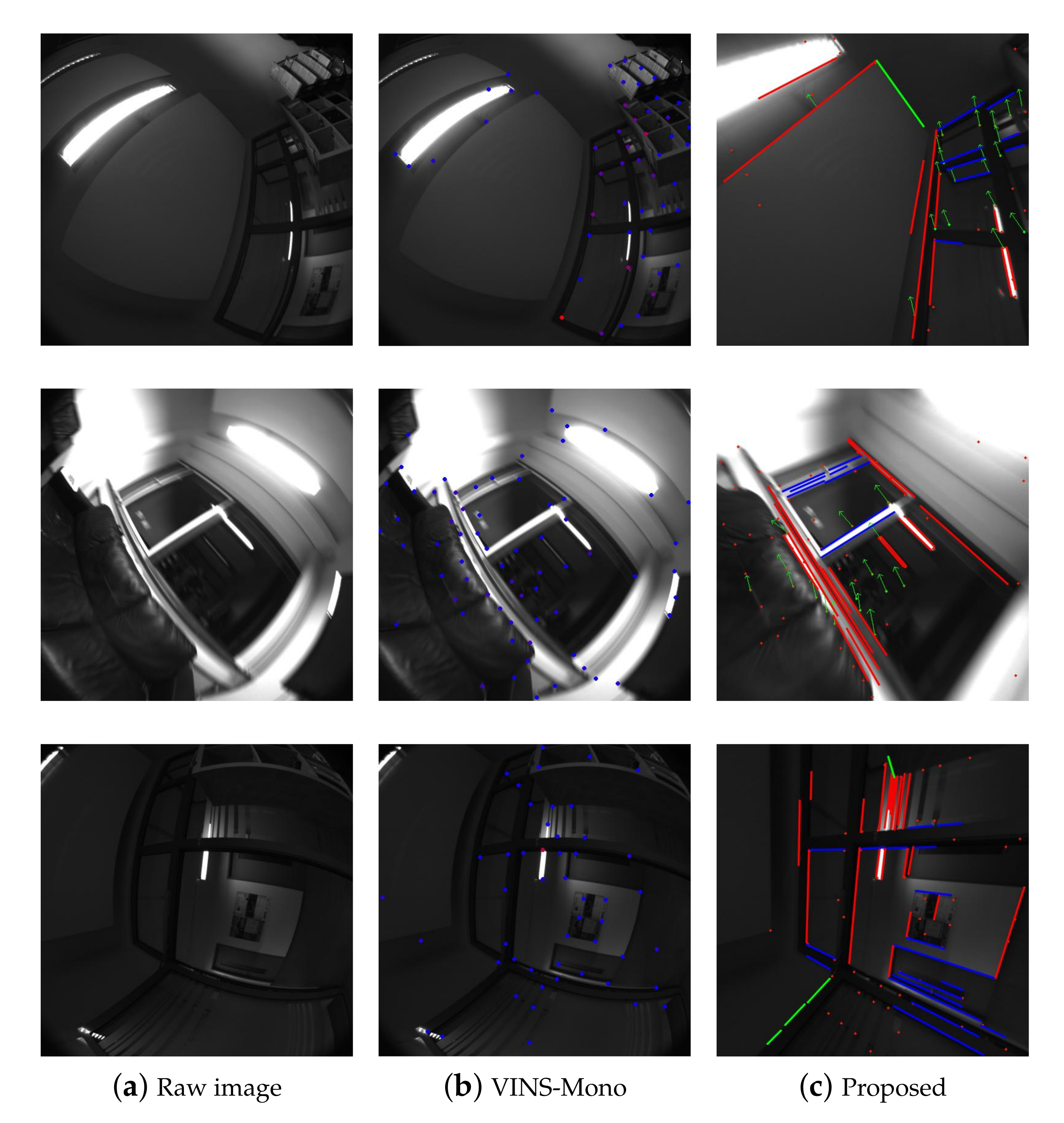
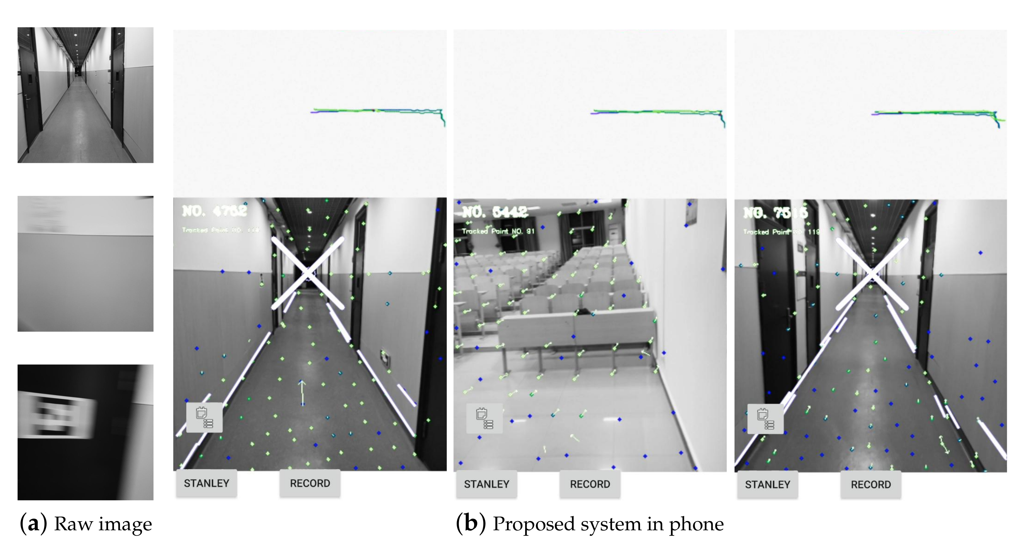
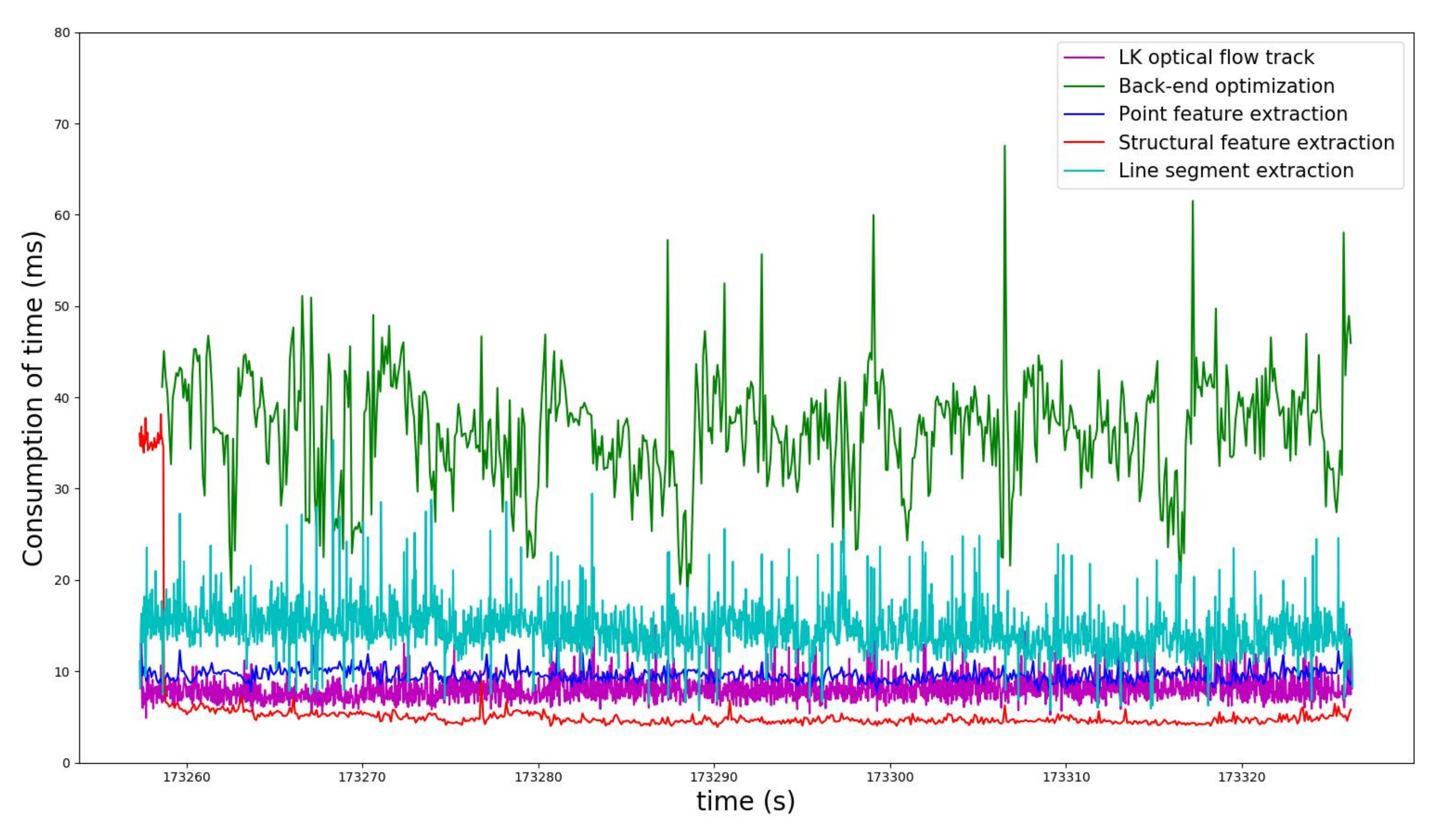
The TUM-VI dataset [45] is composed of 28 sequences collected in 6 different scenes. In order to verify the algorithmic performance of our proposed VIO system, we used the corridor scene, which satisfies our assumptions of the Manhattan world. The TUM-VI dataset provides ground truth from a motion capture system at the start and end of the sequences. We chose 512 × 512 resolution images and used the default parameters provided by the TUM-VI dataset to evaluate other open-sourced systems. Our parameters are consistent with those of VINS-Mono.

This scene has texture-less regions, illumination changes, and other factors that affect the precision of pose estimation. As shown in Figure 8, when the camera is in pure rotation motion Figure 8a or a scene with texture-less region Figure 8b and light changes Figure 8c, our system can use structural features to represent the three dominant directions of the corridor to eliminate the accumulated pose error.

Figure 8. In the scenes of texture-less region, light change, and pure rotation motion, pose estimation method based on point features are easily affected. In contrast, structural features provide scene structure information, an excellent supplement to the point-features based approach.

Consistent with the analysis method of the EuRoC dataset in Section 5.1.1, RMSE of translation and rotation after the estimated trajectory aligned with the ground truth is given, respectively, as shown in Table 2 and Figure 9. It is important to note that the aligned parts are only the start and end of the sequences. It is mentioned in [33] that pose RMSE calculated in this way is about half of the accumulated drift.

Table 2. The root mean square error (RMSE) of translation and rotation in the corridor sequences of the TUM-VI dataset. The results of the top 2 translation and rotation performances are represented in bold.

Seq.		OKVIS		VINS-Mono		PL-VIO		ORB-SLAM3		Proposed
		Trans.	Rot.	Trans.	Rot.	Trans.	Rot.	Trans.	Rot.	Trans.	Rot.
corridor1		0.565	2.403	0.591	1.831	1.206	1.748	0.316${}^2$	0.315${}^2$	0.133${}^1$	0.166${}^1$
corridor2		0.434	1.045	0.951	0.640	1.716	0.502	0.017${}^1$	0.023${}^1$	0.291${}^2$	0.366${}^2$
corridor3		0.457	1.063	1.334	0.555	1.465	0.498	0.278${}^2$	0.084${}^1$	0.258${}^1$	0.150${}^2$
corridor4		0.234	0.557	0.310	0.455	0.234${}^2$	0.391	0.255	0.130${}^1$	0.117${}^1$	0.131${}^2$
corridor5		0.387	0.545	0.723	0.235	0.682	0.268	0.071${}^1$	0.084${}^1$	0.151${}^2$	0.092${}^2$

Figure 9. The line charts represent root mean square error (RMSE) of translation and rotation in the TUM-VI dataset.

As shown in Table 2 and Figure 9, our proposed VIO system is significantly better than other open-source systems based on slide-window optimization. In addition to the corridor1 and corridor5 sequences, our translation performance is superior to ORB-SLAM3 without loop closure among the other sequences. In the corridor sequence, except for the three dominant directions of the corridor itself, there are few outlier line segments that belong to other directions in the image, which leaves us less noise of structural feature measurement. Some scenes with texture-less regions in the corridor pose a significant challenge to the point features-based system, but they have little impact on systems based on structural features. At the same time, it can be seen from the pose errors of PL-VIO that the addition of line feature residuals to the optimization items may bring adverse effects.

In Figure 10, we show the result of each system in the corridor1 sequence. We use our proposed system as a reference trajectory for alignment. As shown in Figure 10a, except for ORB-SLAM3 and our proposed system, the other methods have an apparent Z-axis drift. From Figure 10b, it can be seen that the Z-axis drift of PL-VIO and VINS-Mono significantly increase from 220s onwards. We check the motion state of the camera around this time and find the camera moves rapidly in a texture-less room. As shown in Figure 11, most point features are lost in VINS-Mono and our system due to darkness and image blur at this moment. However, our structural features are well extracted. Our system can still measure and correct rotation according to the structural features in this scene, thus reducing the Z-axis drift.

Figure 10. The performance of each system in the corridor1 sequence is shown in the figure. We give the estimated trajectory and side view of each system after alignment, and we give the curve of Z-axis translation versus time.

Figure 11. The feature extraction performance of VINS-Mono and our proposed system when the camera does fast motion. In VINS-Mono, the blue point features represent the lost track.

5.2. Field Test

We also carried out experiments on a mobile phone to compare the performance of various systems. We evaluated the performance of each system by walking back and forth along the same straight line in a 48-meter corridor scene. Because of the limitation of not having expensive motion capture devices, we strictly tried our best to restrict the position and height of the phone to make sure that the phone was moving along a straight line and at a steady height (along the line on the floor). For real-time performance, we used 480 × 480 resolution images to conduct experiments on the phone. Simultaneously, we collected 640 × 640 resolution images from the mobile phone to do offline experiments to compare the system performances. As shown in Figure 12a, our movement in the corridor is different from that in the TUM-VI dataset. We turn more quickly, which makes images very blurred. Figure 12b shows how our system works on a mobile phone in real-time.

Figure 12. Subfigure (a) are images we collect in the corridor using an Android phone. It can be seen that texture-less area and the image blur appear in our experiment. Subfigure (b) shows the real-time operation of our system on the mobile phone, where the top of the image is the estimated trajectory. As can be seen, after we walk back and forth along the corridor three times, the trajectory is still in a straight line.

For a more intuitive comparison, we compare our trajectory with those estimated trajectories by other systems in Figure 13a. It can be seen in Figure 13b that after walking back and forth twice, the cumulated angle drift of our proposed system is significantly smaller than those of other methods. Moreover, the reduction of angle drift also makes the Z-axis drift of our system much smaller than those of other systems. In our corridor sequence, ORB-SLAM3 has the most significant drift. Because point features are wholly lost when we turn quickly, the continuity of the local map is broken. PL-VIO is second only to our proposed system, indicating that line features create useful constraints in our environment.

Figure 13. We show the estimated trajectories of other systems aligned with our trajectory and show the translation of the Z-axis of each system trajectory in time and space, respectively.

We also record the elapsed time of each major module while the phone is running, as shown in Figure 14. As can be seen from the cyan curve, even using EDline [43], the fastest line segment detector, it still takes 18 ms on average to extract on the mobile phone. At the same time, the red curve represents the elapsed time of structure feature extraction. It can be seen that when the global structural feature is not initialized, the method in [34] is used to extract the vanishing points in three directions, and the elapsed time is about 36 ms. After the successful initialization, the proposed structural feature extraction method can reach below 6 ms.

Figure 14. The time consumption of each main module in the mobile terminal.

6. Conclusions and Future Works

In this work, we propose a novel tightly-coupled monocular vision-inertial odometry, which is based on the sliding window optimization method. The property of the structural feature is incorporated into the residual term for tightly-coupled optimization. The method is effective in the Manhattan world where the structural feature as a global measurement can constrain the rotation error, and thus improve the translation accuracy of the system. When considering the noise in extracting the structural feature, we take the global structure feature as the state variable, and update it on the rotation manifold. The performance of our system has been tested on two benchmark datasets and the field tests. Both of the results show that the proposed system is superior to the listed mainstream open-source systems based on sliding window optimization. We achieve higher precision in some sequences than the ORB-SLAM3 without loop closure, especially in the situations when the images are texture-less, dark, and blurry. In order to achieve low computation complexity, we further propose to quickly extract structural features based on the known vertical dominant direction. With the improvements, the VIO system we proposed can run in real-time on a mobile phone and the whole extraction process can be completed within 6 ms on the tested mobile phone.

With respect to future work, it has been noticed that there are cases of the Atlanta world (AW) [46], which consists of multiple Manhattan worlds with the same vertical dominant direction. How to optimize rotation error with multiple structural features in the Atlanta world will be left to future research.

References

1. Groves, P.D. Principles of GNSS, inertial, and multisensor integrated navigation systems, [Book review]. IEEE Aerosp. Electron. Syst. Mag. 2015, 30, 26–27. [Google Scholar] [CrossRef]
2. Hess, W.; Kohler, D.; Rapp, H.; Andor, D. Real-time loop closure in 2D LIDAR SLAM. In Proceedings of the IEEE International Conference on Robotics and Automation (ICRA), Stockholm, Sweden, 16–21 May 2016; pp. 1271–1278. [Google Scholar]
3. Heng, L.; Choi, B.; Cui, Z.; Geppert, M.; Hu, S.; Kuan, B.; Liu, P.; Nguyen, R.; Yeo, Y.C.; Geiger, A.; et al. Project AutoVision: Localization and 3D Scene Perception for an Autonomous Vehicle with a Multi-Camera System. In Proceedings of the International Conference on Robotics and Automation (ICRA), Montreal, QC, Canada, 20–24 May 2019; pp. 4695–4702. [Google Scholar]
4. Sun, K.; Mohta, K.; Pfrommer, B.; Watterson, M.; Liu, S.; Mulgaonkar, Y.; Taylor, C.J.; Kumar, V. Robust Stereo Visual Inertial Odometry for Fast Autonomous Flight. IEEE Robot. Autom. Lett. 2018, 3, 965–972. [Google Scholar] [CrossRef]
5. Qin, T.; Pan, J.; Cao, S.; Shen, S. A General Optimization-based Framework for Local Odometry Estimation with Multiple Sensors. arXiv 2019, arXiv:1901.03638. [Google Scholar]
6. Chen, L.; Thevenon, P.; Seco-Granados, G.; Julien, O.; Kuusniemi, H. Analysis on the TOA tracking with DVB-T signals for positioning. IEEE Trans. Broadcast. 2016, 62, 957–961. [Google Scholar] [CrossRef]
7. Chen, L.; Yang, L.L.; Yan, J.; Chen, R. Joint wireless positioning and emitter identification in DVB-T single frequency networks. IEEE Trans. Broadcast. 2017, 63, 577–582. [Google Scholar] [CrossRef]
8. Chen, L.; Thombre, S.; Järvinen, K.; Lohan, E.S.; Alén-Savikko, A.; Leppäkoski, H.; Bhuiyan, M.Z.H.; Bu-Pasha, S.; Ferrara, G.N.; Honkala, S.; et al. Robustness, security and privacy in location-based services for future IoT: A survey. IEEE Access 2017, 5, 8956–8977. [Google Scholar] [CrossRef]
9. Zhou, X.; Chen, L.; Yan, J.; Chen, R. Accurate DOA Estimation With Adjacent Angle Power Difference for Indoor Localization. IEEE Access 2020, 8, 44702–44713. [Google Scholar] [CrossRef]
10. Meilland, M.; Drummond, T.; Comport, A.I. A Unified Rolling Shutter and Motion Blur Model for 3D Visual Registration. In Proceedings of the IEEE International Conference on Computer Vision (ICCV), Sydney, Australia, 1–8 December 2013; pp. 2016–2023. [Google Scholar]
11. Liu, H.; Zhang, G.; Bao, H. Robust Keyframe-based Monocular SLAM for Augmented Reality. In Proceedings of the IEEE International Symposium on Mixed and Augmented Reality (ISMAR), Merida, Mexico, 19–23 September 2016; pp. 1–10. [Google Scholar]
12. Piao, J.C.; Kim, S. Adaptive Monocular Visual–Inertial SLAM for Real-Time Augmented Reality Applications in Mobile Devices. Sensors 2017, 17, 2567. [Google Scholar] [CrossRef]
13. Li, P.; Qin, T.; Hu, B.; Zhu, F.; Shen, S. Monocular Visual-Inertial State Estimation for Mobile Augmented Reality. In Proceedings of the IEEE International Symposium on Mixed and Augmented Reality (ISMAR), Nantes, France, 9–13 October 2017; pp. 11–21. [Google Scholar]
14. Mourikis, A.I.; Roumeliotis, S.I. A Multi-State Constraint Kalman Filter for Vision-aided Inertial Navigation. In Proceedings of the International Conference on Robotics and Automation (ICRA), Roma, Italy, 10–14 April 2007; pp. 3565–3572. [Google Scholar]
15. Murartal, R.; Montiel, J.M.M.; Tardos, J.D. ORB-SLAM: A Versatile and Accurate Monocular SLAM System. IEEE Trans. Robot. 2015, 31, 1147–1163. [Google Scholar] [CrossRef]
16. Qin, T.; Li, P.; Shen, S. VINS-Mono: A Robust and Versatile Monocular Visual-Inertial State Estimator. IEEE Trans. Robot. 2018, 34, 1004–1020. [Google Scholar] [CrossRef]
17. Pumarola, A.; Vakhitov, A.; Agudo, A.; Sanfeliu, A.; Morenonoguer, F. PL-SLAM: Real-time monocular visual SLAM with points and lines. In Proceedings of the IEEE International Conference on Robotics and Automation (ICRA), Singapore, 29 May–3 June 2017; pp. 4503–4508. [Google Scholar]
18. Gomez-Ojeda, R.; Zuiga-Nol, D.; Moreno, F.A.; Scaramuzza, D.; Gonzalez-Jimenez, J. PL-SLAM: A Stereo SLAM System through the Combination of Points and Line Segments. IEEE Trans. Robot. 2017, 35, 734–746. [Google Scholar] [CrossRef]
19. Yijia, H.; Zhao, J.; Guo, Y.; He, W.; Yuan, K. PL-VIO: Tightly-Coupled Monocular Visual-Inertial Odometry Using Point and Line Features. Sensors 2018, 18, 1159. [Google Scholar]
20. Coughlan, J.; Yuille, A.L. Manhattan World: Compass direction from a single image by Bayesian inference. In Proceedings of the IEEE International Conference on Computer Vision (ICCV), Kerkyra, Greece, 20–27 September 1999; 2, pp. 941–947. [Google Scholar]
21. Hartley, R.; Zisserman, A. Multiple View Geometry in Computer Vision; Cambridge University Press: Cambridge, UK, 2003. [Google Scholar]
22. Camposeco, F.; Pollefeys, M. Using vanishing points to improve visual-inertial odometry. In Proceedings of the IEEE International Conference on Robotics and Automation (ICRA), Seattle, WA, USA, 26–30 May 2015; pp. 5219–5225. [Google Scholar]
23. Zhou, H.; Zou, D.; Pei, L.; Ying, R.; Liu, P.; Yu, W. StructSLAM: Visual SLAM With Building Structure Lines. IEEE Trans. Veh. Technol. 2015, 64, 1364–1375. [Google Scholar] [CrossRef]
24. Li, H.; Yao, J.; Bazin, J.; Lu, X.; Xing, Y.; Liu, K. A Monocular SLAM System Leveraging Structural Regularity in Manhattan World. In Proceedings of the IEEE International Conference on Robotics and Automation (ICRA), Brisbane, Australia, 21–25 May 2018; pp. 2518–2525. [Google Scholar]
25. Li, Y.; Brasch, N.; Wang, Y.; Navab, N.; Tombari, F. Structure-SLAM: Low-Drift Monocular SLAM in Indoor Environments. IEEE Robot. Autom. Lett. 2020, 5, 6583–6590. [Google Scholar] [CrossRef]
26. Liu, J.; Meng, Z. Visual SLAM With Drift-Free Rotation Estimation in Manhattan World. IEEE Robot. Autom. Lett. 2020, 5, 6512–6519. [Google Scholar] [CrossRef]
27. Kim, P.; Coltin, B.; Kim, H.J. Low-drift visual odometry in structured environments by decoupling rotational and translational motion. In Proceedings of the IEEE International Conference on Robotics and Automation (ICRA), Brisbane, Australia, 21–25 May 2018; pp. 7247–7253. [Google Scholar]
28. Guo, R.; Peng, K.; Zhou, D.; Liu, Y. Robust visual compass using hybrid features for indoor environments. Electronics 2019, 8, 220. [Google Scholar] [CrossRef]
29. Zhou, Y.; Kneip, L.; Rodriguez, C.; Li, H. Divide and conquer: Efficient density-based tracking of 3D sensors in Manhattan worlds. In Proceedings of the Asian Conference on Computer Vision (ACCV), Taipei, Taiwan, 20–24 November 2016; pp. 3–19. [Google Scholar]
30. Bloesch, M.; Omari, S.; Hutter, M.; Siegwart, R. Robust visual inertial odometry using a direct EKF-based approach. In Proceedings of the IEEE/RSJ International Conference on Intelligent Robots and Systems (IROS), Hamburg, Germany, 28 September–2 October 2015; pp. 298–304. [Google Scholar]
31. Murartal, R.; Tardos, J.D. Visual-Inertial Monocular SLAM With Map Reuse. IEEE Robot. Autom. Lett. 2017, 2, 796–803. [Google Scholar] [CrossRef]
32. Leutenegger, S.; Lynen, S.; Bosse, M.; Siegwart, R.; Furgale, P. Keyframe-based visual-inertial odometry using nonlinear optimization. Int. J. Robot. Res. 2015, 34, 314–334. [Google Scholar] [CrossRef]
33. Campos, C.; Elvira, R.; Rodríguez, J.J.G.; Montiel, J.M.; Tardós, J.D. ORB-SLAM3: An accurate open-source library for visual, visual-inertial and multi-map SLAM. arXiv 2020, arXiv:2007.11898. [Google Scholar]
34. Lu, X.; Yaoy, J.; Li, H.; Liu, Y. 2-Line Exhaustive Searching for Real-Time Vanishing Point Estimation in Manhattan World. In Proceedings of the IEEE Winter Conference on Applications of Computer Vision (WACV), Santa Rosa, CA, USA, 24–31 March 2017; pp. 345–353. [Google Scholar]
35. Aguilera, D.; Lahoz, J.G.; Codes, J.F. A new method for vanishing points detection in 3D reconstruction from a single view. In Proceedings of the ISPRS Comission, Vienna, Austria, 29–30 August 2005. [Google Scholar]
36. Tardif, J. Non-iterative approach for fast and accurate vanishing point detection. In Proceedings of the IEEE International Conference on Computer Vision (ICCV), Kyoto, Japan, 29 September–2 October 2009; pp. 1250–1257. [Google Scholar]
37. Bazin, J.; Pollefeys, M. 3-line RANSAC for orthogonal vanishing point detection. In Proceedings of the IEEE/RSJ International Conference on Intelligent Robots and Systems (IROS), Vilamoura, Portugal, 7–12 October 2012; pp. 4282–4287. [Google Scholar]
38. Chatterjee, A.; Govindu, V.M. Efficient and Robust Large-Scale Rotation Averaging. In Proceedings of the IEEE International Conference on Computer Vision (ICCV), Tokyo, Japan, 3–7 November 2013; pp. 521–528. [Google Scholar]
39. Furgale, P.; Rehder, J.; Siegwart, R. Unified temporal and spatial calibration for multi-sensor systems. In Proceedings of the IEEE/RSJ International Conference on Intelligent Robots and Systems (IROS), Sydney, Australia, 1–8 December 2013; pp. 1280–1286. [Google Scholar]
40. Sola, J. Quaternion kinematics for the error-state Kalman filter. arXiv 2017, arXiv:1711.02508. [Google Scholar]
41. Lucas, B.D.; Kanade, T. An iterative image registration technique with an application to stereo vision. In Proceedings of the International Joint Conference on Artificial Intelligence (IJCAI), Vancouver, BC, Canada, 24–28 August 1981; pp. 674–679. [Google Scholar]
42. Rosten, E.; Porter, R.; Drummond, T. Faster and better: A machine learning approach to corner detection. IEEE Trans. Pattern Anal. Mach. Intell. 2008, 32, 105–119. [Google Scholar] [CrossRef] [PubMed]
43. Akinlar, C.; Topal, C. EDLines: A real-time line segment detector with a false detection control. Pattern Recognit. Lett. 2011, 32, 1633–1642. [Google Scholar] [CrossRef]
44. Burri, M.; Nikolic, J.; Gohl, P.; Schneider, T.; Rehder, J.; Omari, S.; Achtelik, M.W.; Siegwart, R. The EuRoC micro aerial vehicle datasets. Int. J. Robot. Res. 2016, 35, 1157–1163. [Google Scholar] [CrossRef]
45. Schubert, D.; Goll, T.; Demmel, N.; Usenko, V.; Stückler, J.; Cremers, D. The TUM VI benchmark for evaluating visual-inertial odometry. In Proceedings of the IEEE/RSJ International Conference on Intelligent Robots and Systems (IROS), Madrid, Spain, 1–5 October 2018; pp. 1680–1687. [Google Scholar]
46. Schindler, G.; Dellaert, F. Atlanta world: An expectation maximization framework for simultaneous low-level edge grouping and camera calibration in complex man-made environments. In Proceedings of the IEEE Conference on Computer Vision and Pattern Recognition (CVPR), Washington, DC, USA, 27 June–2 July 2004; p. I. [Google Scholar]
Publisher’s Note: MDPI stays neutral with regard to jurisdictional claims in published maps and institutional affiliations.
Article Metrics
Citations
Article Access Statistics
Multiple requests from the same IP address are counted as one view.