Continuity of MODIS and VIIRS Snow Cover Extent Data Products for Development of an Earth Science Data Record

Abstract
1. Introduction
2. Materials
2.1. MODIS and VIIRS Instruments and Satellites
2.2. MODIS and VIIRS Snow Cover Products
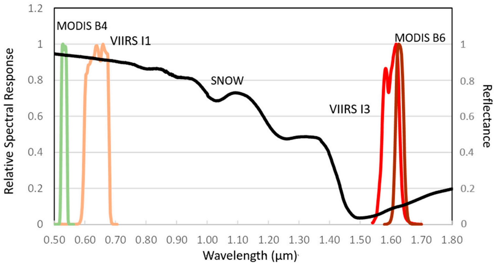
2.3. Snow Cover Detection Algorithm
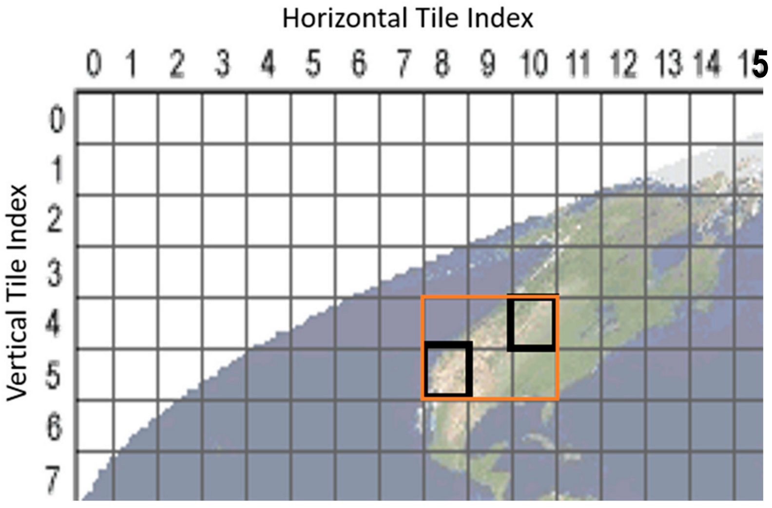
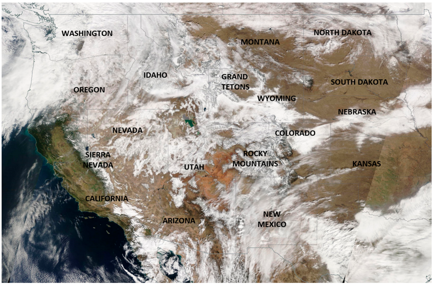
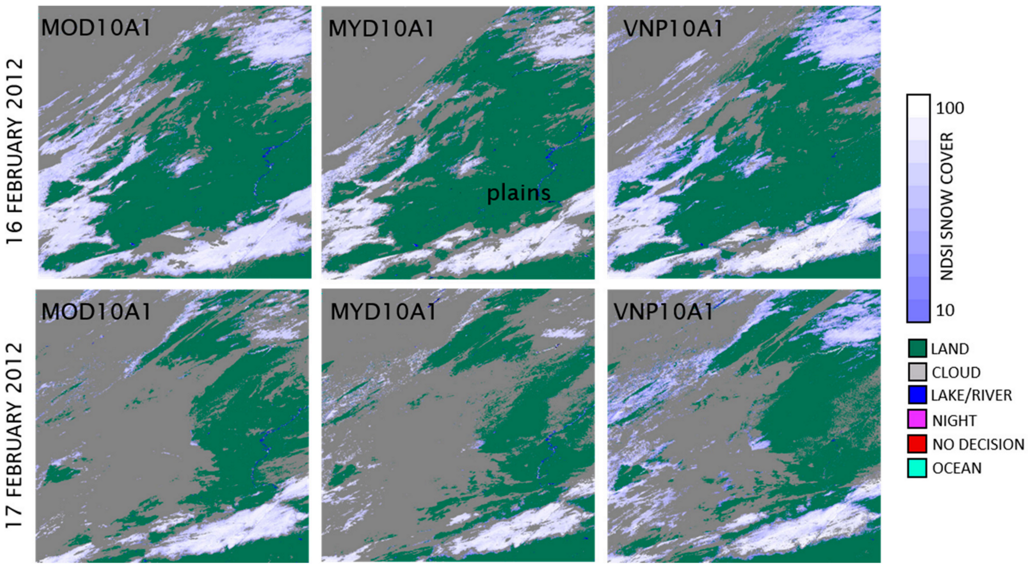
2.4. Study Region
3. Methodology
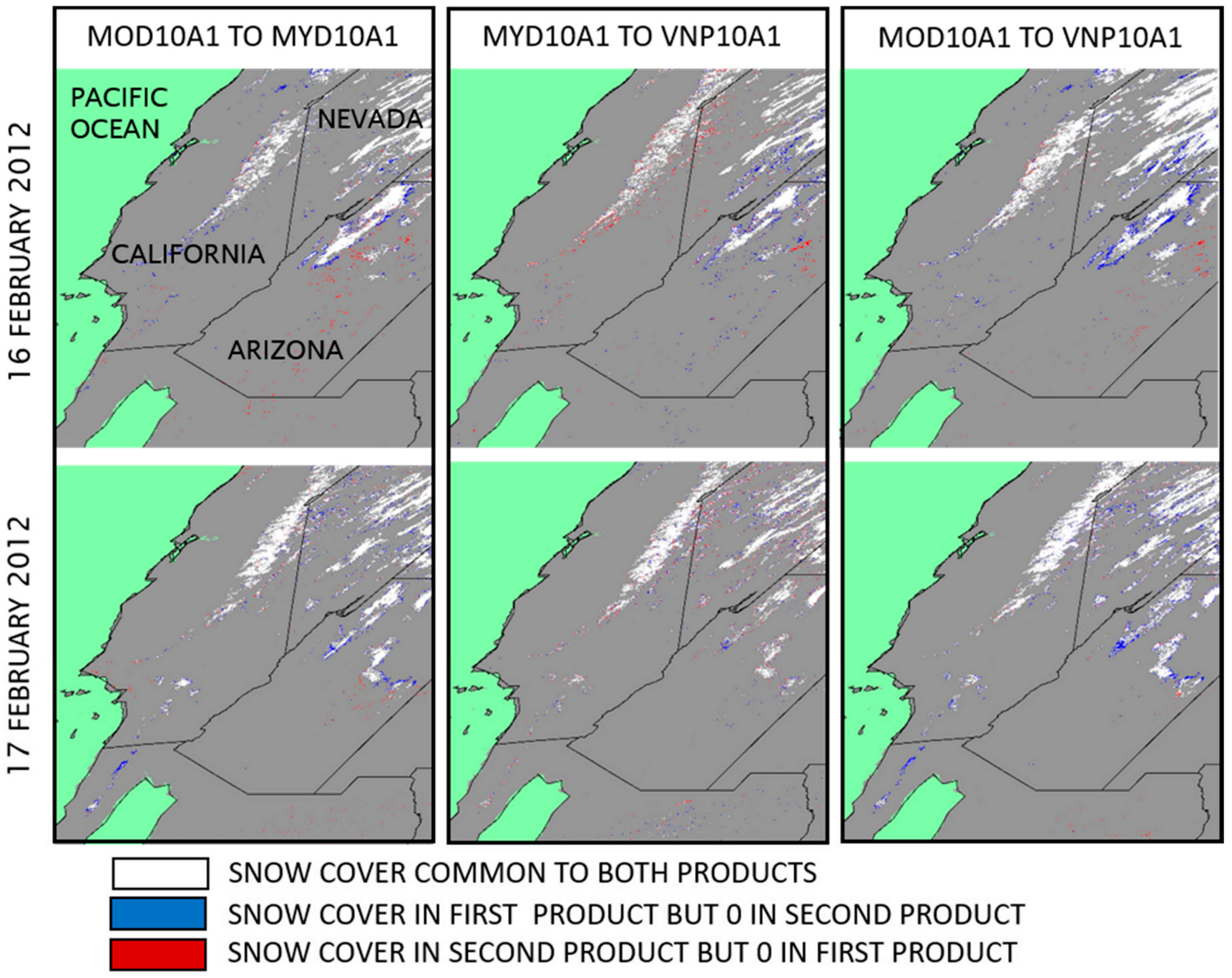
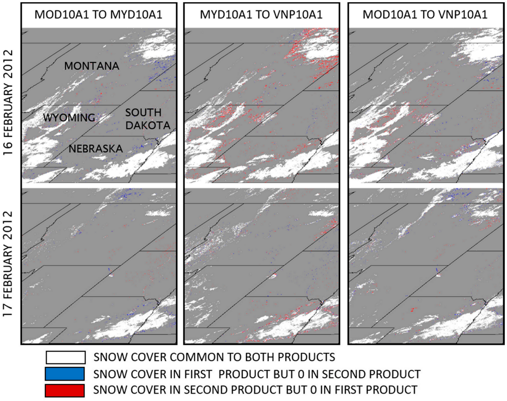
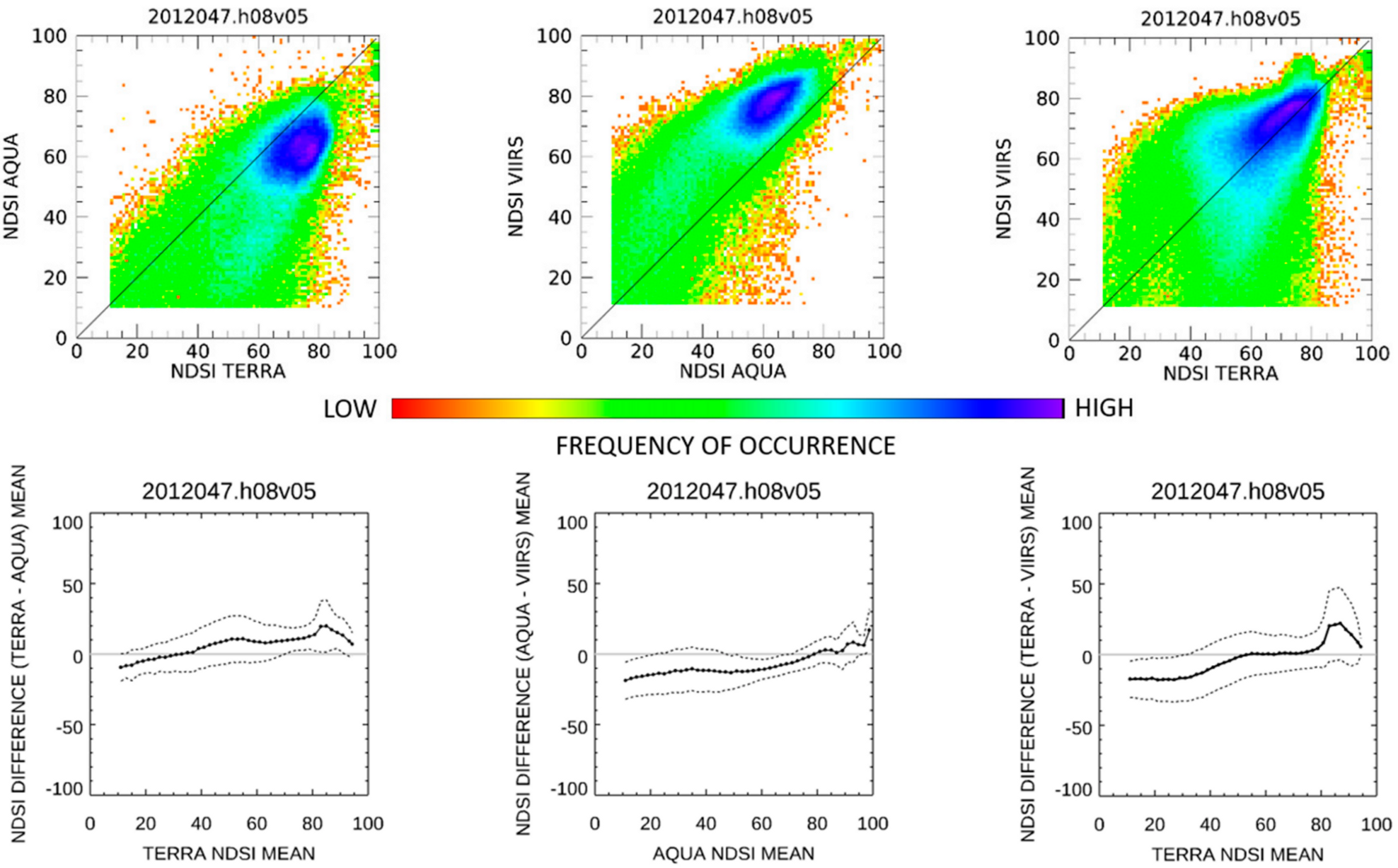
4. Results and Discussion
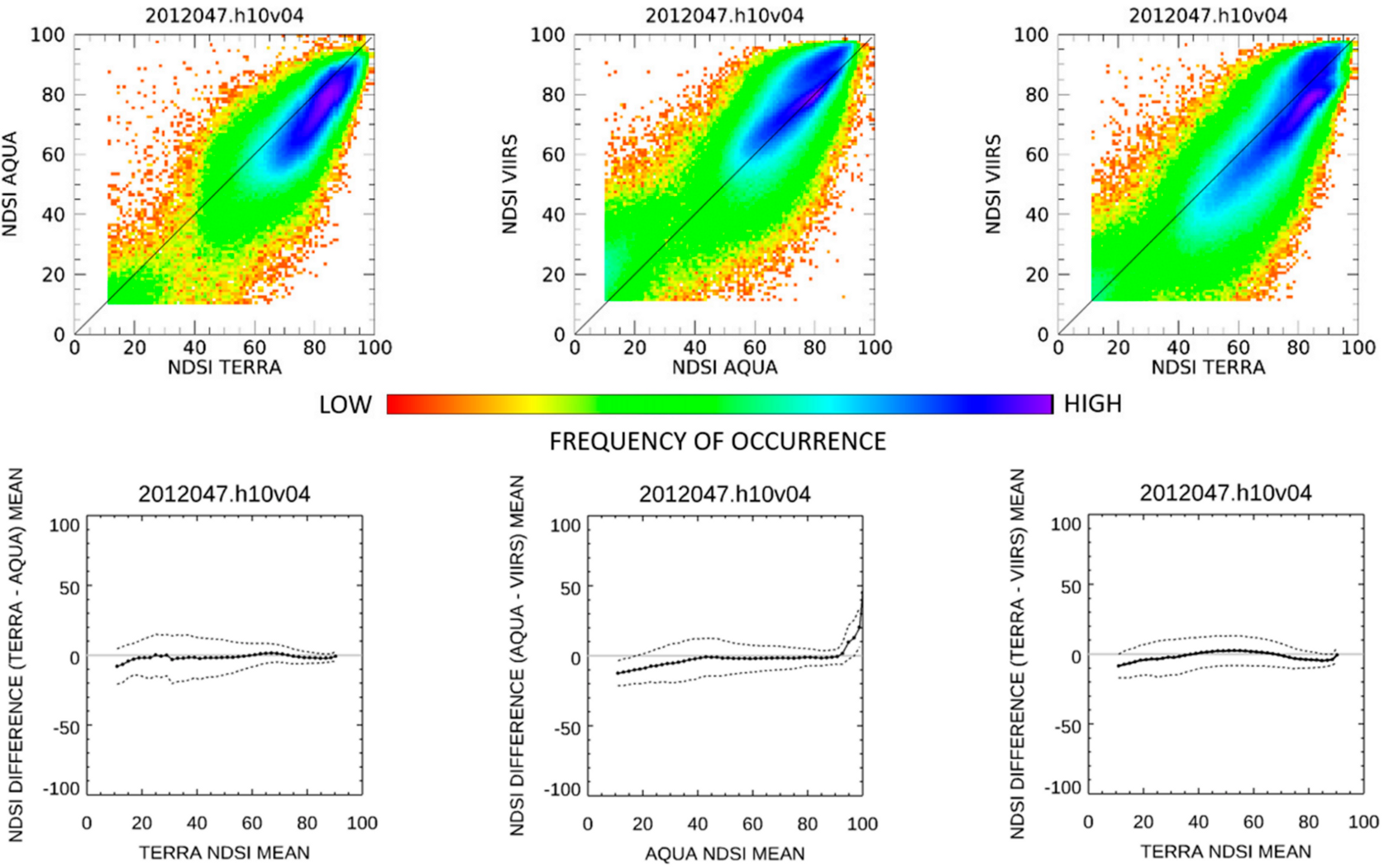
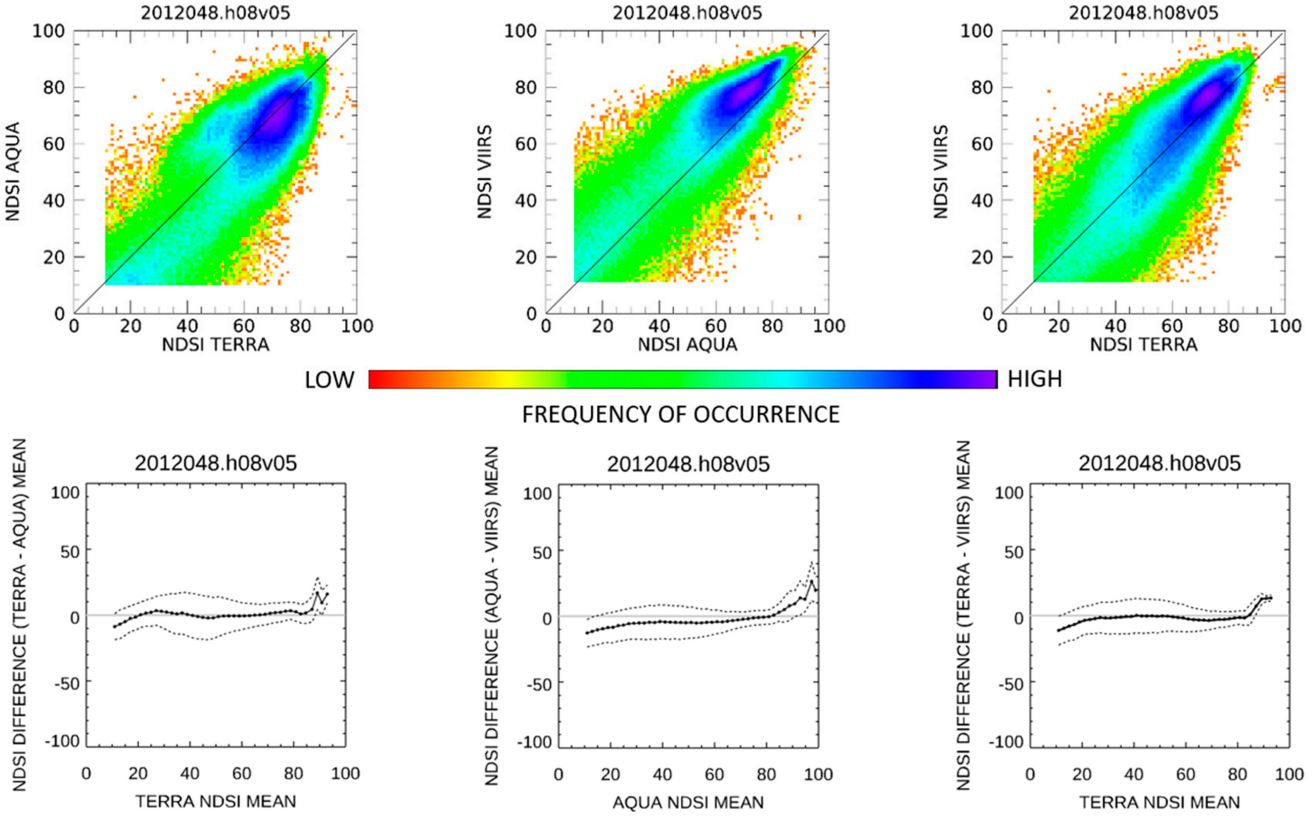
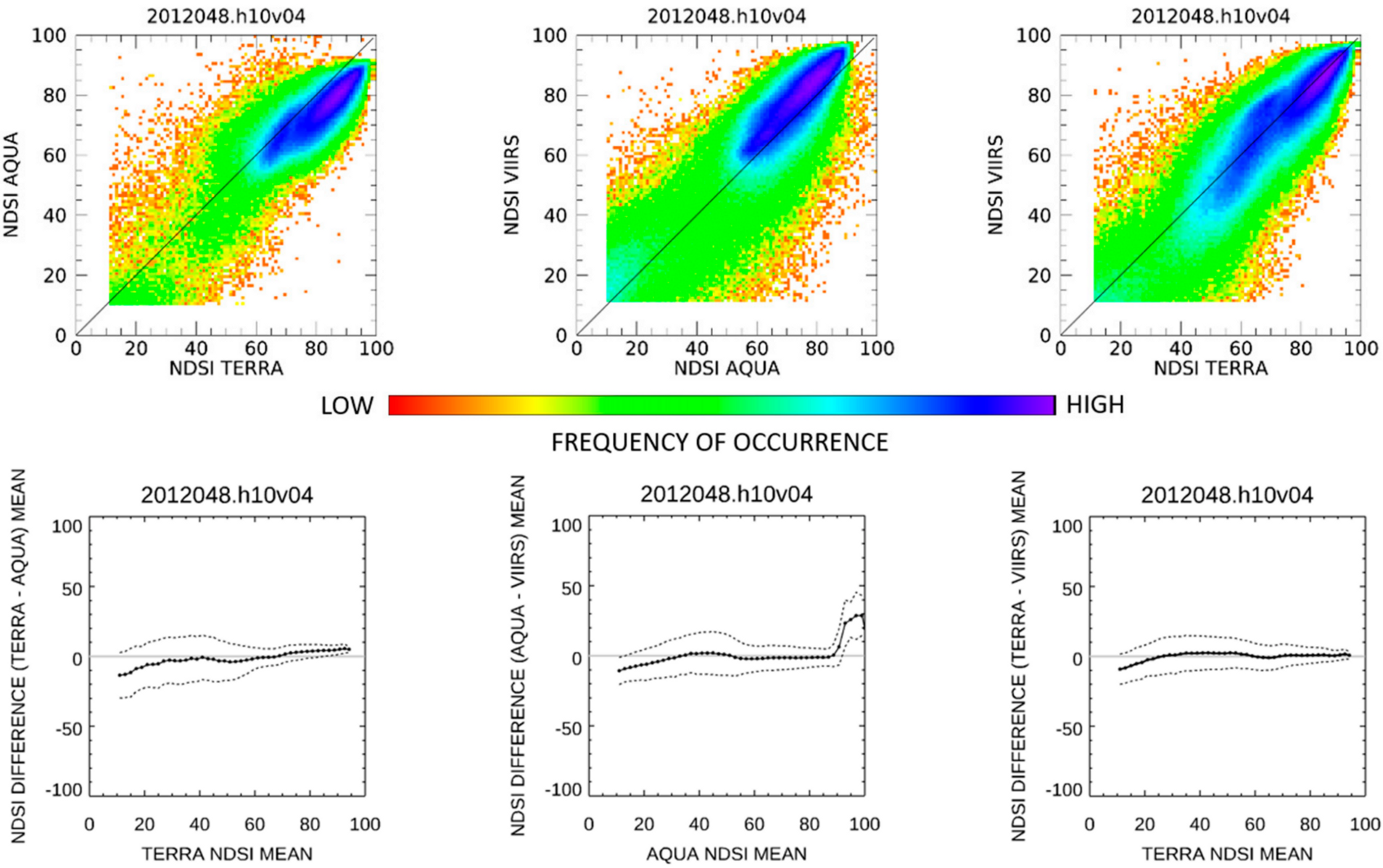
4.1. MODIS to VIIRS Comparison
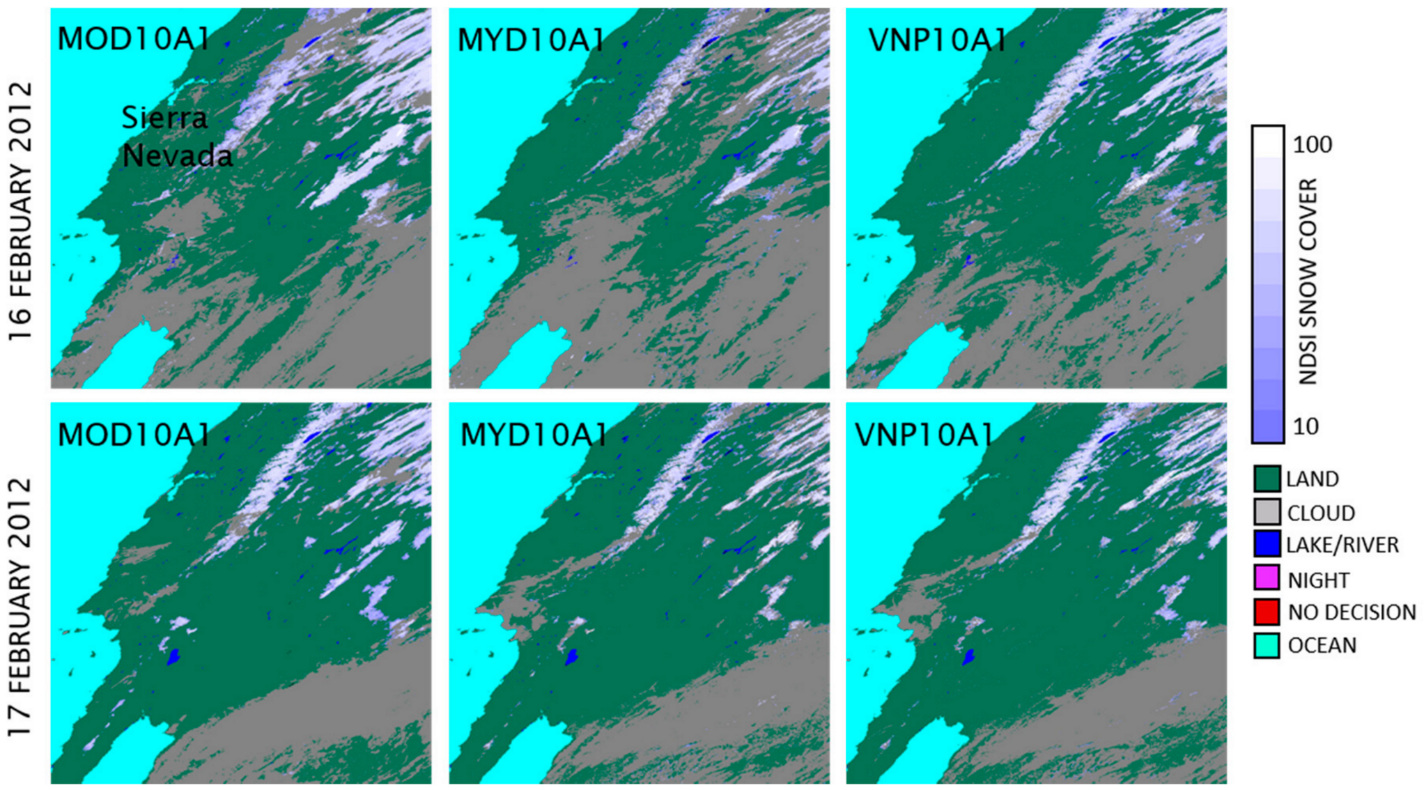
4.2. Comparison of 1 km Gridded SCE
4.3. Cloud Masking
5. Conclusions
Author Contributions
Funding
Acknowledgments
Conflicts of Interest
References
- GCOS. The Global Climate Observing System. Available online: https://gcos.wmo.int/en/essential-climate-variables/snow/ecv-requirements (accessed on 16 June 2020).
- National Academies of Sciences, E. Thriving on Our Changing Planet: A Decadal Strategy for Earth Observation from Space; The National Academies Press: Washington, DC, USA, 2018; ISBN 9780309467575. [Google Scholar]
- Rutgers University Global Snow Lab. Available online: https://climate.rutgers.edu/snowcover/ (accessed on 20 August 2020).
- Hammond, J.C.; Saavedra, F.A.; Kampf, S.K. Global snow zone maps and trends in snow persistence 2001-2016. Int. J. Clim. 2018, 38, 4369–4383. [Google Scholar] [CrossRef]
- Derksen, C.; Brown, R.D. Spring snow cover extent reductions in the 2008–2012 period exceeding climate model projections: Spring snow cover extent reductions. Geophys. Res. Lett. 2012, 39, L19504. [Google Scholar] [CrossRef]
- Román, M.O.; Justice, C.; Csiszar, I.; Key, J.R.; Devadiga, S.; Davidson, C.; Wolfe, R.; Privette, J. Pre-launch evaluation of the NPP VIIRS Land and Cryosphere EDRs to meet NASA’s science requirements. In Proceedings of the 2011 IEEE International Geoscience and Remote Sensing Symposium, Vancouver, BC, Canada, 24–29 July 2011; pp. 154–157. [Google Scholar] [CrossRef]
- Pahlevan, N.; Sarkar, S.; Devadiga, S.; Wolfe, R.E.; Roman, M.; Vermote, E.; Lin, G.; Xiong, X. Impact of spatial sampling on continuity of MODIS–VIIRS land surface reflectance products: A simulation approach. IEEE Trans. Geosci. Remote. Sens. 2016, 55, 183–196. [Google Scholar] [CrossRef]
- Justice, C.; Román, M.O.; Csiszar, I.; Vermote, E.F.; Wolfe, R.E.; Hook, S.J.; Friedl, M.; Wang, Z.; Schaaf, C.B.; Miura, T.; et al. Land and cryosphere products from Suomi NPP VIIRS: Overview and status: Status of S-NPP VIIRS land/cryo products. J. Geophys. Res. Atmos. 2013, 118, 9753–9765. [Google Scholar] [CrossRef] [PubMed]
- Saavedra, F.; Kampf, S.K.; Fassnacht, S.R.; Sibold, J.S. A snow climatology of the Andes Mountains from MODIS snow cover data: A snow climatology of the Andes Mountains. Int. J. Clim. 2016, 37, 1526–1539. [Google Scholar] [CrossRef]
- Dietz, A.J.; Wohner, C.; Kuenzer, C. European snow cover characteristics between 2000 and 2011 derived from improved MODIS daily snow cover products. Remote. Sens. 2012, 4, 2432–2454. [Google Scholar] [CrossRef]
- Bevington, A.R.; Gleason, H.E.; Foord, V.N.; Floyd, W.C.; Griesbauer, H.P. Regional influence of ocean–atmosphere teleconnections on the timing and duration of MODIS-derived snow cover in British Columbia, Canada. Cryosphere 2019, 13, 2693–2712. [Google Scholar] [CrossRef]
- Gascoin, S.; Hagolle, O.; Huc, M.; Jarlan, L.; Dejoux, J.; Szczypta, C.; Marti, R.; Sánchez, R. A snow cover climatology for the Pyrenees from MODIS snow products. Hydrol. Earth Syst. Sci. 2015, 19, 2337–2351. [Google Scholar] [CrossRef]
- Gunnarsson, A.; Garðarsson, S.M.; Sveinsson, Ó.G.B. Icelandic snow cover characteristics derived from a gap-filled MODIS daily snow cover product. Hydrol. Earth Syst. Sci. 2019, 23, 3021–3036. [Google Scholar] [CrossRef]
- Tomaszewska, M.A.; Henebry, G.M. Changing snow seasonality in the highlands of Kyrgyzstan. Environ. Res. Lett. 2018, 13, 065006. [Google Scholar] [CrossRef]
- Malmros, J.K.; Mernild, S.H.; Wilson, R.; Tagesson, T.; Fensholt, R. Snow cover and snow albedo changes in the central Andes of Chile and Argentina from daily MODIS observations (2000–2016). Remote. Sens. Environ. 2018, 209, 240–252. [Google Scholar] [CrossRef]
- Dariane, A.B.; Khoramian, A.; Santi, E. Investigating spatiotemporal snow cover variability via cloud-free MODIS snow cover product in Central Alborz Region. Remote. Sens. Environ. 2017, 202, 152–165. [Google Scholar] [CrossRef]
- NOAA STAR Calibration Center. VIIRS SDR User’s Guide. Available online: https://ncc.nesdis.noaa.gov/documents/documentation/viirs-users-guide-tech-report-142a-v1.3.pdf. (accessed on 21 August 2020).
- Wolfe, R.E.; Lin, G.; Nishihama, M.; Tewari, K.P.; Montano, E. NPP VIIRS Early On-Orbit Geometric Performance. In Proceedings of the SPIE Volume 8510, Earth Observing Systems XVII, San Diego, CA, USA, 15 October 2012. [Google Scholar] [CrossRef]
- Hall, D.K.; Riggs, G.A. MODIS/Terra Snow Cover Daily L3 Global 500m SIN Grid; National Snow and Ice Data Center: Boulder, CO, USA, 2015; Available online: http://nsidc.org/the-drift/data-update/modis-swath-500-m-gridded-snow-cover-data-now-available-in-version-6/ (accessed on 16 November 2020).
- Riggs, G.A.; Hall, D.K.; Román, M.O. NASA S-NPP VIIRS Snow Cover Products Collection 1 (C1) User Guide. Available online: https://nsidc.org/sites/nsidc.org/files/technical-references/VIIRS_snow_products_user_guide_version_8.pdf (accessed on 17 June 2020).
- Suomi NPP VIIRS Land Validation. Available online: https://viirsland.gsfc.nasa.gov/Val_overview.html (accessed on 21 August 2020).
- MODIS Land Validation. Status for: Snow Cover/Sea Ice (MOD10/29). Available online: https://modis-land.gsfc.nasa.gov/ValStatus.php?ProductID=MOD10/29 (accessed on 21 August 2020).
- Suomi NPP VIIRS Land. VIIRS NASA Snow Cover Product Validation. Available online: https://viirsland.gsfc.nasa.gov/Val/Snow_Val.html (accessed on 21 August 2020).
- Hall, D.K.; Riggs, G.A.; DiGirolamo, N.E.; Román, M.O. Evaluation of MODIS and VIIRS cloud-gap-filled snow-cover products for production of an Earth science data record. Hydrol. Earth Syst. Sci. 2019, 23, 5227–5241. [Google Scholar] [CrossRef]
- Hall, D.K.; Riggs, G.A. Normalized-difference snow index (NDSI). In Encyclopedia of Snow, Ice and Glaciers; Singh, V.P., Singh, P., Haritashya, U.K., Eds.; Springer: Dordrecht, The Netherlands, 2011; pp. 779–780. ISBN 9789048126415. [Google Scholar]
- Yin, D.; Cao, X.; Chen, X.; Shao, Y.; Chen, J. Comparison of automatic thresholding methods for snow-cover mapping using Landsat TM imagery. Int. J. Remote. Sens. 2013, 34, 6529–6538. [Google Scholar] [CrossRef]
- Mishra, V.D.; Negi, H.S.; Rawat, A.K.; Chaturvedi, A.; Singh, R.P. Retrieval of sub-pixel snow cover information in the Himalayan region using medium and coarse resolution remote sensing data. Int. J. Remote. Sens. 2009, 30, 4707–4731. [Google Scholar] [CrossRef]
- Kolberg, S.; Gottschalk, L. Interannual stability of grid cell snow depletion curves as estimated from MODIS images: Stability of distributed snow depletion. Water Resour. Res. 2010, 46, 7617. [Google Scholar] [CrossRef]
- Jain, S.K.; Goswami, A.; Saraf, A.K. Accuracy assessment of MODIS, NOAA and IRS data in snow cover mapping under Himalayan conditions. Int. J. Remote. Sens. 2008, 29, 5863–5878. [Google Scholar] [CrossRef]
- MCST MODIS Characterization Support Team, Calibration, Parameters, MODIS Terra (PFM) Merged Relative Spectral Response (RSR) Tables—IB & OOB. Available online: https://mcst.gsfc.nasa.gov/calibration/parameters[Dataset] (accessed on 2 September 2020).
- STAR JPSS. STAR Joint Polar Satellite System Website, VIIRS Documentation, NG Band-Averaged RSRs. Available online: https://www.star.nesdis.noaa.gov/jpss/VIIRS.php[Dataset]NG_VIIRS_NPP_RSR_filtered_Oct2011_BA.zip (accessed on 2 September 2020).
- Heinilä, K.; Böttcher, K.; Mattila, O.P.; Spectrometer Measurements of Snow and Bare Ground Targets and Simultaneous Measurements of Snow Conditions (Version 1.0.0) [Data Set]. Zenodo. Available online: http://doi.org/10.5281/zenodo.3580825 (accessed on 2 September 2020).
- Hannula, H.R.; Heinilä, K.; Böttcher, K.; Mattila, O.-P.; Salminen, M.; Pulliainen, J. Laboratory, field, mast-borne and airborne spectral reflectance measurements of boreal landscape during spring. Earth Syst. Sci. Data 2020, 12, 719–740. [Google Scholar] [CrossRef]
- Riggs, G.A.; Hall, D.K. MODIS Snow Products Collection 6 User Guide. Available online: https://nsidc.org/sites/nsidc.org/files/files/MODIS-snow-user-guide-C6.pdf. (accessed on 17 June 2020).
- NOAA. National Centers for Environmental Information, State of the Climate: Global Snow and Ice. Available online: https://www.ncdc.noaa.gov/sotc/global-snow/201202 (accessed on 30 January 2020).
- Skakun, S.; Justice, C.O.; Vermote, E.; Roger, J.C. Transitioning from MODIS to VIIRS: An analysis of inter-consistency of NDVI data sets for agricultural monitoring. Int. J. Remote. Sens. 2018, 39, 971–992. [Google Scholar] [CrossRef]
- Vargas, M.; Miura, T.; Shabanov, N.; Kato, A. An initial assessment of Suomi NPP VIIRS vegetation index EDR: Suomi NPP VIIRS vegetation index EDR. J. Geophys. Res. Atmos. 2013, 118, 301–312, 316. [Google Scholar] [CrossRef]
- Moon, M.; Zhang, X.; Henebry, G.M.; Liu, L.; Gray, J.M.; Melaas, E.K.; Friedl, M.A. Long-term continuity in land surface phenology measurements: A comparative assessment of the MODIS land cover dynamics and VIIRS land surface phenology products. Remote. Sens. Environ. 2019, 226, 74–92. [Google Scholar] [CrossRef]
- Miura, T.; Muratsuchi, J.; Vargas, M. Assessment of cross-sensor vegetation index compatibility between VIIRS and MODIS using near-coincident observations. J. Appl. Remote. Sens. 2018, 12, 045004-1. [Google Scholar] [CrossRef]
- Liu, Y.; Wang, Z.; Sun, Q.; Erb, A.M.; Li, Z.; Schaaf, C.B.; Zhang, X.; Román, M.O.; Scott, R.L.; Zhang, Q.; et al. Evaluation of the VIIRS BRDF, Albedo and NBAR products suite and an assessment of continuity with the long term MODIS record. Remote. Sens. Environ. 2017, 201, 256–274. [Google Scholar] [CrossRef]
- Townshend, J.R.G.; Huang, C.; Kalluri, S.N.V.; DeFries, R.S.; Liang, S.; Yang, K. Beware of per-pixel characterization of land cover. Int. J. Remote. Sens. 2000, 21, 839–843. [Google Scholar] [CrossRef]
- Huang, C.; Townshend, J.R.; Liang, S.; Kalluri, S.N.; DeFries, R.S. Impact of sensor’s point spread function on land cover characterization: Assessment and deconvolution. Remote. Sens. Environ. 2002, 80, 203–212. [Google Scholar] [CrossRef]
- Strabala, K. MODIS Cloud Mask User’s Guide. Available online: https://atmosphere-imager.gsfc.nasa.gov/sites/default/files/ModAtmo/CMUSERSGUIDE_0.pdf (accessed on 17 June 2020).
- Frey, R.A.; Ackerman, S.A.; Liu, Y.; Strabala, K.I.; Zhang, H.; Key, J.; Wang, X. Cloud Detection with MODIS. Part I: Improvements in the MODIS Cloud Mask for Collection 5. J. Atmospheric Ocean. Technol. 2008, 25, 1057–1072. [Google Scholar] [CrossRef]
- Ackerman, S.A.; Holz, R.E.; Frey, R.; Eloranta, E.W.; Maddux, B.C.; McGill, M. Cloud Detection with MODIS. Part II: Validation. J. Atmospheric Ocean. Technol. 2008, 25, 1073–1086. [Google Scholar] [CrossRef]
- Ackerman, S.A.; Frey, R.; Strabala, K.; Liu, Y.; Gumley, L.; Baum, B.; Menzel, P. Discrimination clear-sky from cloud with MODIS Algorithm Theoretical Basis Document (MOD35). Available online: https://atmosphere-imager.gsfc.nasa.gov/sites/default/files/ModAtmo/MOD35_ATBD_Collection6_0.pdf (accessed on 17 June 2020).
- Atmosphere Discipline Team Imager Products, Cloud Mask. Available online: https://atmosphere-imager.gsfc.nasa.gov/products/cloud-mask (accessed on 24 August 2020).
- Frey, R.; Ackerman, S.; Holz, R.; Dutcher. The Continuity MODIS-VIIRS Cloud Mask (MVCM) User’s Guide. 2019. Available online: https://atmosphere-imager.gsfc.nasa.gov/sites/default/files/ModAtmo/MODIS_VIIRS_Cloud-Mask_UG_Feb_2019.pdf (accessed on 17 June 2020).
- Riggs, G.A.; Hall, D.K.; Román, M.O. Overview of NASA’s MODIS and Visible Infrared Imaging Radiometer Suite (VIIRS) snow-cover Earth System Data Records. Earth Syst. Sci. Data 2017, 9, 765–777. [Google Scholar] [CrossRef]
- Gladkova, I.; Grossberg, M.; Bonev, G.; Romanov, P.; Shahriar, F. Increasing the accuracy of MODIS/aqua snow product using quantitative image restoration technique. IEEE Geosci. Remote. Sens. Lett. 2012, 9, 740–743. [Google Scholar] [CrossRef]


| MODIS Terra | MODIS Aqua | VIIRS S-NPP | VIIRS-NOAA-20 | |
|---|---|---|---|---|
| Orbit | Near-polar, sun-synchronous | Near-polar, sun-synchronous | Near-polar, sun-synchronous | Near-polar, sun-synchronous |
| Altitude | 705 km | 705 km | 824 km | 824 km |
| Equator crossing time | 10:30 am (descending) | 1:30 pm (ascending) | 1:30 pm (ascending) | 1:30 pm (ascending) |
| Coverage * | daily | daily | daily | daily |
| Swath width | 2330 km (±55° scan angle) | 2330 km (±55° scan angle) | 3060 km (±56° scan angle) | 3060 km (±56° scan angle) |
| Spatial resolution | VIS and NIR, 500 m at nadir | VIS and NIR, 500 m at nadir | VIS and NIR 375 m at nadir | VIS and NIR 375 m at nadir |
| Spectral bands (µm) | VIS B4, 0.555 NIR B6, 1.640 | VIS B4, 0.555 NIR B6, 1.640 | VIS I1, 0.640 NIR I3 1.610 | VIS I1, 0.640 NIR I3 1.610 |
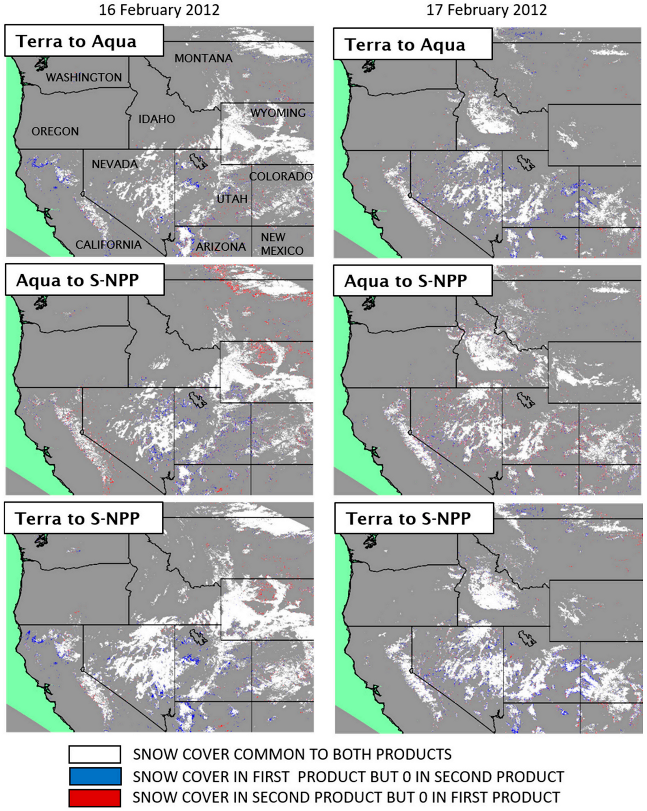
| Paired Comparisons | Tile h08v05 | ||
| 16 February 2012 | 17 February 2012 | ||
| Terra to Aqua | Terra only SCE | 14.6 % | 15.5 % |
| Aqua only SCE | 6.2 % | 4.8 % | |
| Aqua to S-NPP | Aqua only SCE | 14.3 % | 12.5 % |
| SNPP only SCE | 9.7 % | 8.5 % | |
| Terra to S-NPP | Terra only SCE | 14.3 % | 16.9 % |
| S-NPP only SCE | 2.4 % | 2.7 % | |
| Paired Comparisons | Tile h10v04 | ||
| 16 February 2012 | 17 February 2012 | ||
| Terra to Aqua | Terra only SCE | 2.6 % | 4.3 % |
| Aqua only SCE | 1.9 % | 2.1 % | |
| Aqua to S-NPP | Aqua only SCE | 1.0 % | 3.1 % |
| S-NPP only SCE | 7.9 % | 5.5 % | |
| Terra to S-NPP | Terra only SCE | 1.5 % | 4.2 % |
| S-NPP only SCE | 2.4 % | 2.3 % | |
| Paired Comparisons | CMG (1 km) | ||
|---|---|---|---|
| 16 February 2012 | 17 February 2012 | ||
| Terra to Aqua | Terra only SCE | 5.2 % | 9.9 % |
| Aqua only SCE | 1.9 % | 2.3 % | |
| Aqua to S-NPP | Aqua only SCE | 5.9 % | 5.3 % |
| S-NPP only SCE | 6.1 % | 5.5 % | |
| Terra to S-NPP | Terra only SCE | 5.1 % | 9.3 % |
| S-NPP only SCE | 1.5 % | 2.2 % | |
Publisher’s Note: MDPI stays neutral with regard to jurisdictional claims in published maps and institutional affiliations. |
© 2020 by the authors. Licensee MDPI, Basel, Switzerland. This article is an open access article distributed under the terms and conditions of the Creative Commons Attribution (CC BY) license (http://creativecommons.org/licenses/by/4.0/).
Share and Cite
Riggs, G.; Hall, D. Continuity of MODIS and VIIRS Snow Cover Extent Data Products for Development of an Earth Science Data Record. Remote Sens. 2020, 12, 3781. https://doi.org/10.3390/rs12223781
Riggs G, Hall D. Continuity of MODIS and VIIRS Snow Cover Extent Data Products for Development of an Earth Science Data Record. Remote Sensing. 2020; 12(22):3781. https://doi.org/10.3390/rs12223781
Chicago/Turabian StyleRiggs, George, and Dorothy Hall. 2020. "Continuity of MODIS and VIIRS Snow Cover Extent Data Products for Development of an Earth Science Data Record" Remote Sensing 12, no. 22: 3781. https://doi.org/10.3390/rs12223781
APA StyleRiggs, G., & Hall, D. (2020). Continuity of MODIS and VIIRS Snow Cover Extent Data Products for Development of an Earth Science Data Record. Remote Sensing, 12(22), 3781. https://doi.org/10.3390/rs12223781