Article

The Google Earth Engine Mangrove Mapping Methodology (GEEMMM)

1
Blue Ventures Conservation—Mezzanine, The Old Library, Trinity Road, St Jude’s, Bristol BS2 0NW, UK
2
Department of Forest Resources Management, University of British Columbia, Vancouver, BC V6T 1Z4, Canada
3
Terra Spatialists, The Blue House, 660 West 13th Avenue, Vancouver, BC V5Z 1N9, Canada
4
The Jolly Geographer, 7 Yorke Gate, Watford, Hertfordshire WD17 4NQ, UK
5
Department of Geography, University of Victoria, P.O. Box 1700 STN CSC, Victoria, BC V8W 2Y2, Canada
*
Author to whom correspondence should be addressed.
Remote Sens. 2020, 12(22), 3758; https://doi.org/10.3390/rs12223758
Submission received: 1 October 2020 / Revised: 6 November 2020 / Accepted: 9 November 2020 / Published: 16 November 2020
(This article belongs to the Special Issue Remote Sensing in Mangroves)

Abstract

:
Mangroves are found globally throughout tropical and sub-tropical inter-tidal coastlines. These highly biodiverse and carbon-dense ecosystems have multi-faceted value, providing critical goods and services to millions living in coastal communities and making significant contributions to global climate change mitigation through carbon sequestration and storage. Despite their many values, mangrove loss continues to be widespread in many regions due primarily to anthropogenic activities. Accessible, intuitive tools that enable coastal managers to map and monitor mangrove cover are needed to stem this loss. Remotely sensed data have a proven record for successfully mapping and monitoring mangroves, but conventional methods are limited by imagery availability, computing resources and accessibility. In addition, the variable tidal levels in mangroves presents a unique mapping challenge, particularly over geographically large extents. Here we present a new tool—the Google Earth Engine Mangrove Mapping Methodology (GEEMMM)—an intuitive, accessible and replicable approach which caters to a wide audience of non-specialist coastal managers and decision makers. The GEEMMM was developed based on a thorough review and incorporation of relevant mangrove remote sensing literature and harnesses the power of cloud computing including a simplified image-based tidal calibration approach. We demonstrate the tool for all of coastal Myanmar (Burma)—a global mangrove loss hotspot—including an assessment of multi-date mapping and dynamics outputs and a comparison of GEEMMM results to existing studies. Results—including both quantitative and qualitative accuracy assessments and comparisons to existing studies—indicate that the GEEMMM provides an accessible approach to map and monitor mangrove ecosystems anywhere within their global distribution.

Graphical Abstract

1. Introduction

Mangroves are a species of woody plants which comprise unique, halophytic communities in the tropical and sub-tropical inter-tidal coastlines of the world [1]. When meeting accepted definitions based on attributes including height, diameter and canopy closure, mangroves can qualify as forest [2]. Areas not qualifying as forest are peripheral parts of wider mangrove ecosystems, including expanses dominated by submerged, dwarf or scrub, and fringe plants [1,3,4,5]. Mangrove ecosystems —both forest and non-forest—are found in 102 countries and 21 territories [5]. The value of mangrove ecosystems is multifaceted, including the provisioning of critical goods (e.g., fuel wood, fish, shellfish, medicine, fiber, and timber) and services (e.g., shoreline stabilization, storm protection, and cultural, recreational and tourism opportunities) to millions of people residing in coastal communities [6,7,8,9]. In addition, mangrove ecosystems are incredibly biodiverse, providing habitat for numerous species, many of which are rare, at-risk, or endangered [10,11,12]. Mangrove forests are also incredibly carbon-dense and meet or exceed many of their terrestrial peers in sequestration and storage [13,14,15]. Increasingly, the conservation, restoration and managed-use of mangrove ecosystems is being pursued through payments for ecosystem services (PES) programs, including forest carbon initiatives (e.g., REDD+, Plan Vivo) [16,17].
Despite their multifaceted value, global mangrove loss is widespread. In the last two decades of the 20th century the world lost an estimated 35% of mangrove forest cover [18]. While globally the rate of loss has thus far slowed in the 21st century—an estimated 4% from 1996 to 2016—many parts of the world, notably SE Asia, remain loss hotspots [19,20,21]. The primary driver of mangrove loss is anthropogenic activities including aquaculture, agriculture, urban development, and unmanaged harvest [22]. Accurate, reliable, contemporary, and easily updated information representing the extent of mangrove ecosystems is required by decision makers and managers and to help countries pursue and meet environmental targets (e.g., Millennium Development Goals and Ramsar Convention on Wetlands of International Importance especially as Waterfowl Habitat) [23,24,25]. Remotely sensed data have a well-established utility for mapping and monitoring the multi-date distribution of mangrove ecosystems and quantifying change over time; however, the remote sensing of mangrove environments has its own unique set of challenges which must be overcome to produce accurate results, including the variable presence or absence of water associated with daily tidal fluctuations [23,26]. Fluctuating tides can drastically influence the spectral properties of mangrove ecosystems making information on tidal condition at time of image acquisition vital [27]. Many mangrove studies have ignored variable tidal conditions, combining images ranging from low to high tide [23]. Recently, studies have used image composites that include imagery acquired during selective tides (i.e., high and/or low); however, these have covered limited areas (e.g., a single bay within a single Landsat scene) where reliable local tidal stations or modeled tidal products are available, and have not evaluated dynamics [27,28,29]. Other studies demonstrated the potential to use remote sensing or models to calibrate tides across larger areas; however, these approaches depend on substantial expertise to run specialized or customized software and the models depend on high quality training data—which is not always available—making them too complex and inaccessible for most potential users [30,31,32,33].
Beyond tidal considerations, conventional mapping techniques—while successful and informative—remain limited by imagery availability, required computing resources, and necessary technical expertise [34]. A single uncompressed Landsat 8 scene is larger than 1.6 gigabytes, and applications using multiple scenes require computing resources that present a barrier to many practitioners [35]. Emerging tools and technologies are ushering in a new era for land-cover mapping and monitoring [26,36]. Cloud-based platforms, most notably Google Earth Engine (GEE), provide unprecedented volumes of ready-to-use geospatial data, including the entire Landsat archive (i.e., radiometrically and geometrically corrected), and tool and computing resources for rapid and seamless processing [34]. GEE stores data and completes processing on numerous remote servers (i.e., parallel processing), removing the need to download and process data on local stand-alone computers. This eliminates many barriers related to the hardware and technical expertise required for remote sensing. All that is required to use GEE is a computer capable of running a modern web browser and an internet connection—for development, research, or educational purposes, access is freely granted through Google, LLC (Limited Liability Corporation), by signing up through the GEE Homepage. These advancements allow for developing and carrying out mapping methodologies over unprecedented spatial extents with drastically increased speed (e.g., University of Maryland Global Forest Dynamics), making advanced remote sensing applications accessible to considerably broader audiences [34,37]. In addition, tools built for GEE and distributed over the Internet can facilitate methodological repeatability while providing opportunities for adaptability and customization [38].
To date, several studies have explored and demonstrated the utility of GEE for mapping mangroves yielding encouraging results and improvements over conventional methods [39,40,41,42,43]. While there is clear utility for mapping and monitoring mangrove ecosystems using GEE, published methodologies remain inaccessible to many would-be users. To replicate published methods requires an advanced level of specialized expertise with remote sensing, geospatial processing techniques, and/or coding. To date, no intuitive and accessible version of a mangrove mapping methodology within GEE has been proposed which caters to a wider audience of non-specialist conservation managers and decision makers. In addition, existing tools fail to fully capitalize on the wealth of local knowledge and understanding often held by coastal managers. Lastly, no single methodology comprehensively incorporates all of the best available options for mapping and monitoring mangrove ecosystems from across existing published studies and includes a widely applicable approach toward tidal calibration.
Herein we present a comprehensive, intuitive, accessible, and replicable methodology encapsulated in a new tool—the Google Earth Engine Mangrove Mapping Methodology (i.e., the GEEMMM). The GEEMMM was designed to provide a ready-to-go methodology for non-expert practitioners to map and monitor mangrove ecosystems, enabling them to combine their local knowledge with GEE’s cloud computing capabilities. We developed the GEEMMM following a thorough review of mangrove remote sensing literature and incorporating the best available practices. In addition, our approach to tidal calibration operates completely within GEE based entirely on shoreline reflectance (i.e., image-based). To demonstrate the tool, we present an example of multi-date, desk-based (i.e., involving no field work) mapping and change assessment for Myanmar (Burma)—a global loss hotspot [19]. The GEEMMM—freely accessible to non-profit users—runs on detailed and well commented code within the GEE environment and is adaptable to any mangrove area of interest. GEEMMM outputs include multi-date classified maps, accuracies, and dynamic assessments. To set the stage for trailing the GEEMMM for Myanmar and contextualizing the outputs, and similar to methods detailed in Gandhi and Jones [19], all existing single- and multi-date mangrove maps for Myanmar were inventoried, described, and compared, with an emphasis on existing information on distribution and dynamics. We introduce the pilot area of interest (i.e., AOI), describe existing datasets, overview the GEEMMM tool, and compare the results to existing datasets.

2. Materials and Methods

2.1. Google Earth Engine Mangrove Mapping Methodology (GEEMMM) Pilot AOI

2.1.1. Regional Context

The region encompassing south (S) Asia, southeast (SE) Asia, and Asia-Pacific is home to approximately 46% of the world’s mangroves [5,44]. This region includes some of the world’s most productive, oldest, and biodiverse mangrove forests [45]. Regional loss—the highest in the world—is driven by conversion to aquaculture ponds (i.e., shrimp and fish farms), oil palm plantations and rice paddies, coastal development, and over-extraction for wood [11,46,47,48,49,50,51,52,53,54,55,56,57]. Natural processes and phenomena (e.g., rising ocean temperatures and sea-levels, severe tropical storms, and natural disasters) also contribute to regional dynamics [48,53,56,58,59,60,61,62,63,64,65,66]. Notably, SE Asia is exceptionally biodiverse containing 51 of the world’s 73 documented mangrove species, compared to 10 in the Americas and Africa [5,67]. SE Asia alone contains an estimated 34% of the world’s mangroves [5,68]. Recent studies show that mangrove areas in SE Asia are experiencing the highest prevalence of anthropogenic activity in the world [68,69].

2.1.2. Myanmar—A Regional and Global Loss Hotspot

Located within SE Asia, the preliminary AOI for this pilot study is all of coastal Myanmar (Figure 1). As confirmed by Gandhi and Jones [19], within SE Asia, mangrove loss is most notable in Myanmar, making the country both a regional and global loss hotspot. Giri et al. [70] reported a 35% decrease in mangrove extent from 1975–2005 whereas De Alban et al. [57] reported a 52% decrease from 1996–2016 [57,70]. According to De Alban et al. [57] and Estoque et al. [56], the primary anthropogenic drivers of this loss include conversion to rice paddies, oil palm and rubber plantations, and increasingly for aquaculture (e.g., shrimp, fish) [56,57]. Natural drivers include tsunamis triggered by seismic activity, and tropical storms [68,71,72]. Within Myanmar, according to Giri et al. [70], Saah et al. [73], Bunting et al. [74], De Alban et al. [57], and Clark Labs [75] sub-national loss hotspots include the northwestern (NW) coastline, much of the Ayeyarwady peninsula, and a smaller area slightly east of the Ayeyarwady peninsula (Figure 1).

2.1.3. Myanmar—Inventory, Summary and Acquisition of Existing Datasets

All national-level mangrove datasets providing single- or multi-date coverage for Myanmar up to July 2020 were inventoried through an exhaustive online search and literature review. When available, datasets were obtained from online repositories or through contacting authors. When not available, datasets were described based on associated literature. All datasets were summarized based on producer/organization/reference, single- vs. multi-date, temporal and spatial extent, availability, imagery source(s), mapping methods, and whether discrete or continuous (Table 1).

2.1.4. Myanmar—Comparison of Existing Datasets and Baseline QAA

Once inventoried, all known datasets were compared based on mapped classes, mangrove distribution, accuracy, dynamics (when available), and known limitations. Where provided, mangrove distributions and dynamics were extracted from publications and supporting materials. If not readily apparent—and if the datasets were available—dynamics were calculated. Adding to the standard reported metrics, the accuracy was further qualitatively assessed for all available datasets through cross-checking in reference to high spatial resolution satellite imagery viewable through Google Earth Pro (GEP) [79]. This secondary qualitative accuracy assessment—or QAA—first reported in Gandhi and Jones [19], provides a more thorough understanding of existing mangrove datasets.
The QAA of existing maps (i.e., baseline QAA) was undertaken for the most recent entry in each discrete dataset, when available. Datasets were acquired in both raster and vector format, and in a range of coordinate systems, necessitating several pre-processing steps. For each baseline QAA, three 100 × 100 km sub-national AOIs were selected across Myanmar: in the north (Rakhine), in the center (Ayeyarwady Delta), and in the south (Tanintharyi) (Figure 1). Each baseline QAA AOI was divided into 10 × 10 km boxes, and working from NW to SE, every sixth box was selected for spot-checking, such that approximately 17% was systematically assessed. QAA of the Giri et al. [70] dataset was already conducted [19]. For the remaining datasets, each spot-check entailed comparing mangrove coverage to GEP imagery as close to the dataset’s capture date as possible. In some instances, particularly in the southernmost Tanintharyi AOI, GEP imagery was partly/fully cloud-covered, limiting the ability to conduct QAA (limitations also noted by Estoque et al. [56]). A single mangrove class, representing the variability of canopy cover, height and stand structure in mangrove forests (as used in GEEMMM pilot classifications and defined below) was qualitatively assessed within each spot-check as either well-, under-, or over-represented. For each dataset, results help contextualize the representation of mangrove distribution and dynamics.

2.2. The Google Earth Engine Mangrove Mapping Methodology (GEEMMM)

The GEEMMM is intended to facilitate the mapping and monitoring of mangrove ecosystems anywhere in the world, without requiring a dedicated in-house geospatial expert. Intended users need basic computer skills and an understanding of the key steps required for mapping mangroves, but are not expected to hold advanced expertise in remote sensing, geospatial analysis, and/or coding. The interactive tool is broken into three modules—Module 1: defines customized region of interest (ROI) boundaries and generates multi-date imagery composites; Module 2: examines spectral separation between target map classes and undertakes multi-date classifications and accuracy assessments; Module 3: explores dynamics and offers an optional QAA. Each module is broken into thoroughly commented and referenced sections, bringing the user through all steps while making reference to this manuscript for full methodological details and context. Each module and the parameters used in this pilot study are described below. Table 2 provides a summary of all GEEMMM user inputs and variable selections for the Myanmar pilot study.

2.2.1. Module 1—Defining the ROI and Compositing Imagery

In the first step of Module 1: Section 1, the user must identify key datasets to be used in the GEEMMM. The first user-defined dataset is a preliminary ROI. This is generated using the ‘drawing tools’ function built into GEE and clips all subsequent user-defined datasets. The second user-defined dataset is the known extent of mangroves which is used to calculate elevation and slope thresholds and shoreline buffer distance. The user can select the baseline GEE data set representing global mangrove distribution circa 2000 (i.e., Giri et al. [44]) or upload their own. The third user-defined dataset is coastline, for which the user can select the baseline Large Scale International Boundary Polygons [80] or upload their own. The fourth user-defined dataset concerns elevation which is required to generate topographic masks (i.e., elevation and slope). The user can select the GEE JAXA-ALOS satellite radar DSM (30 m) [81] or upload their own. For the Myanmar pilot, the preliminary ROI is shown in Figure 1, the GEE global mangrove distribution circa 2000 was used for known mangrove extent, the Global Administrative Boundaries database (GADM) Myanmar dataset (v3.6, www.gadm.org, an external source) for coastline, and the GEE JAXA-ALOS Global PALSAR-2/PALSAR Yearly Mosaic 25 m land-cover data for elevation [81,82].
In the second step of Module 1: Section 1, the user defines input variables and sets how workflow thresholds are calculated. Table 2 lists all of the user variables and user inputs for the GEEMMM including those used in this pilot study. GEE provides unprecedented access to the Landsat catalog, offering approximately 1.3 M scenes from 1984 to present [34]. While it is certainly advantageous to have access to so many images, the choice of imagery based on parameters such as year(s) and time of year(s) must be considered carefully. Two variables define contemporary and historic year(s) of interest. There are two four-digit date inputs to bookend the historic and contemporary year windows. If the user wishes to isolate a single historic or contemporary year the same is selected for each book-end. Following the year(s) of interest, the month(s) of interest are selected. Seasonal variations can affect terrestrial vegetation adjacent to mangroves, and atmospheric conditions can change throughout the year, so the ability to target specific months is essential to generating optimal image composites [83,84,85]. The user identifies the month(s)-of-interest using two book-end numbers corresponding to the 12 months of the year; they may overlap the new year; e.g., “11” (Nov.) to “2” (Feb.). Next, the allowable cloud cover limit, an integer between 0 and 100, is used to filter the Landsat metadata [86]. Also related to cloud cover, the user decides whether to mask the imagery, and to what extent, i.e., setting a mild cloud mask using the USGS-provided (United States Geological Survey) quality band, or an aggressive cloud mask where pixels are excluded based on their ‘whiteness’ and a temperature band threshold [35]. For the sixth input, the approximate tidal zone—a numeric input (in m) that represents the tidally active zone buffered inland from the coastline—is entered. Approximate tidal zone helps isolate the portion of images subject to reflectance changes from tidal variation, while reducing influence from other non-tidal variability. The default value is 1000 m. Next, the user chooses how water is masked out of the imagery, either using a mask developed from the water present in the contemporary imagery alone, or a combination mask based on pixels determined to be water in both historic and contemporary imagery. A pixel is determined to be water if its value was greater than the 0.09 modified normalized difference water index (i.e., MNDWI) threshold established by Xu [87]. The modified normalized difference water index (MNDWI) was developed to detect water pixels by calculating the normalized difference between the green and short-wave infrared (e.g., Landsat 8 Operational Land Imager, 1.57–1.65 μm) bands, making it suitable for measuring the amount of water present in an acquisition. Topographic thresholds are set to generate masks based on elevation and slope. The user can either manually enter the elevation (m) and slope (%) thresholds, or have them automatically calculated based on the 99th percentile values extracted from within the known mangrove extent dataset. The user can further opt to search for inland-fringe mangroves, which have been documented as far as 85 km inland [75,88]. If inland-fringe mangroves are targets for the classification(s), the preliminary ROI is doubled for elevations lower than 5 m based on [89]. The last step in Module 1: Section 1 is the selection of spectral indices which the user would like to calculate for each image composite. After the workflow begins, the user chooses which indices they would like to calculate from a list of fourteen indices, including some which are mangrove-specific. The complete list of indices included in the GEEMMM can be found in Table 3. The contemporary and historic windows from which imagery was selected for the Myanmar pilot study were 2014–2018 and 2004–2008, respectively. The months of acquisition were limited to June through December, corresponding with the wet season and the months directly following that time [90]. The imagery was filtered using cloud cover information for each acquisition at a 30% threshold. All 14 spectral indices were selected for calculation.
Module 1: Section 2 determines the finalized ROI for processing. Numerous studies have demonstrated the utility of reducing the classification extent to the minimum required area—this approach helps reduce spectral confusion with unnecessary scene components [44,91]. The preliminary ROI is used to isolate a section of shoreline which is buffered at 5, 10, 15, 20, 25, 30, and 35 km intervals. 5 km intervals were used to ensure observable differences in buffer distances. 35 km was used as a maximum extent based on observations in several countries, including Myanmar. These buffer distances are used to calculate the area of known mangroves that falls within their respective bounds. The user either selects their buffer distance preference from a drop-down menu containing values in between, greater than, or less than the listed intervals.
In either case, the buffer distance is used to create the finalized ROI. This ROI is used to select Landsat path/row tiles and generate image composites, clip composite imagery and masks (i.e., elevation, slope, and water), define the classification and dynamics extent, and provide a visual aid for optional QAAs. The finalized ROI used in the pilot study was based on a 23 km buffered shoreline which represents the maximum observed distance between known mangrove extent (i.e., Giri et al. [44]) and Myanmar’s coastline.
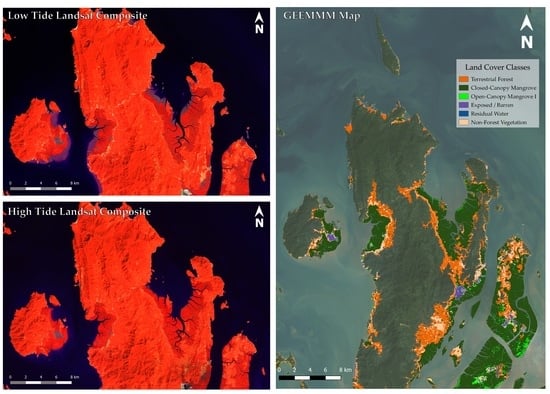
Module 1: Section 3 generates the imagery composites required for multi-date classifications. Given the daily dynamic nature of mangrove ecosystems—wherein tides inundate 2–3 times per day on average—tidal conditions and the associated presence (or lack thereof) of water must be considered—there are a growing number of mangrove detection indices which rely on the isolation of high and low tide imagery [29,92,93]. The GEEMMM uses an image-based approach to calibrate imagery based on high and low tide. For each available image, an MNDWI is generated and the land is masked out using JAXA-ALOS Global PALSAR-2/PALSAR Yearly Mosaic 25 m land-cover data. The MNDWI was selected as the key spectral index because it has been proven to be an improvement over the normalized difference water index (NDWI), and was developed explicitly for detecting water and non-water pixels [87]. The shoreline is buffered to the user-defined tidal zone value and mean MNDWI is used to create a constant value band wherein the greater the MNDWI mean value, the more water present within the tidal zone, corresponding to higher-tidal conditions. A second value band is added to each available image by multiplying mean MNDWI by −1, isolating lower-tide conditions. Clouds, if present and opted to be, are masked prior to the calculation of mean MNDWI using only the pixel quality band or an aggressive approach where the three visible (red, greed, and blue) and thermal bands mask based on digital number reflectance thresholds. Under the aggressive filter, a pixel is considered to be a cloud if its visible spectrum bands digital number reflectance values are greater than or equal to 1850, and the thermal band (brightness temperature, Kelvin) digital number is less than or equal to 2955. For the Myanmar pilot, the aggressive cloud filter option was selected to filter the imagery in an effort to remove low-altitude clouds which were not correctly classified by the Landsat cloud detection algorithm. If/once clouds have been masked, all available images and their corresponding tidal value bands are used to create best available pixel-based highest observable tide (i.e., HOT) and lowest observable tide (i.e., LOT) composites. Composite generation works as if all available images were stacked and organized by desired tidal condition. For example, as the LOT composite is being generated, the imagery with the lowest observed tidal condition is placed on top, and any missing pixels in that image, e.g., clouds masked, would be filled by the next best tidal observation and so on until all the gaps are filled. This process takes place for both the contemporary and historic data sets, resulting in a maximum of four composites (i.e., HOT and LOT contemporary, HOT and LOT historic). Because tides are determined using value bands, it is possible that all of the pixels for HOT and/or LOT composites within a particular area may be from one image (e.g., if no clouds were present and that image represented best available tidal conditions). The GEEMMM employs USGS surface reflectance Landsat products, which are readily available within GEE [35,94].
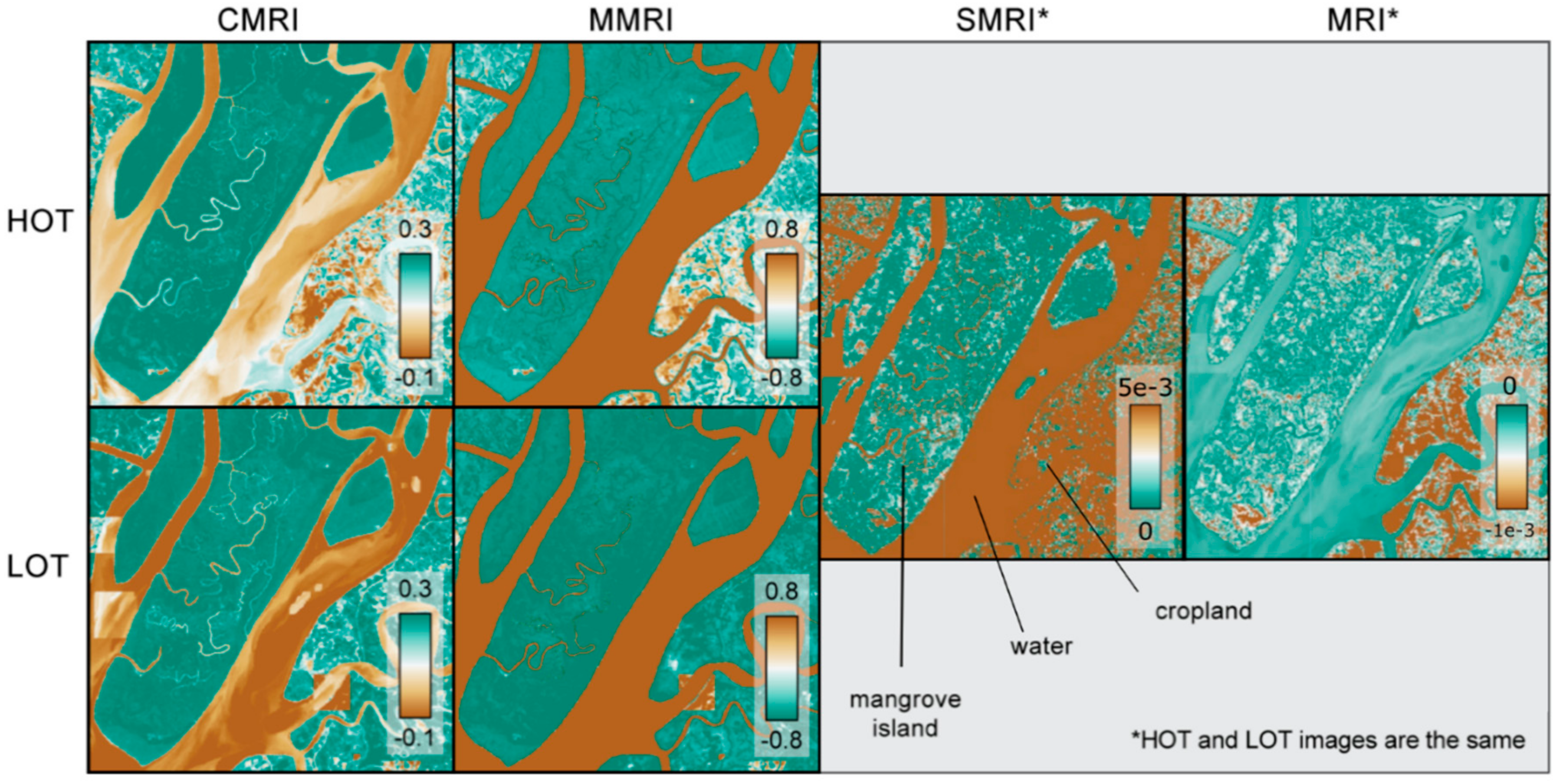
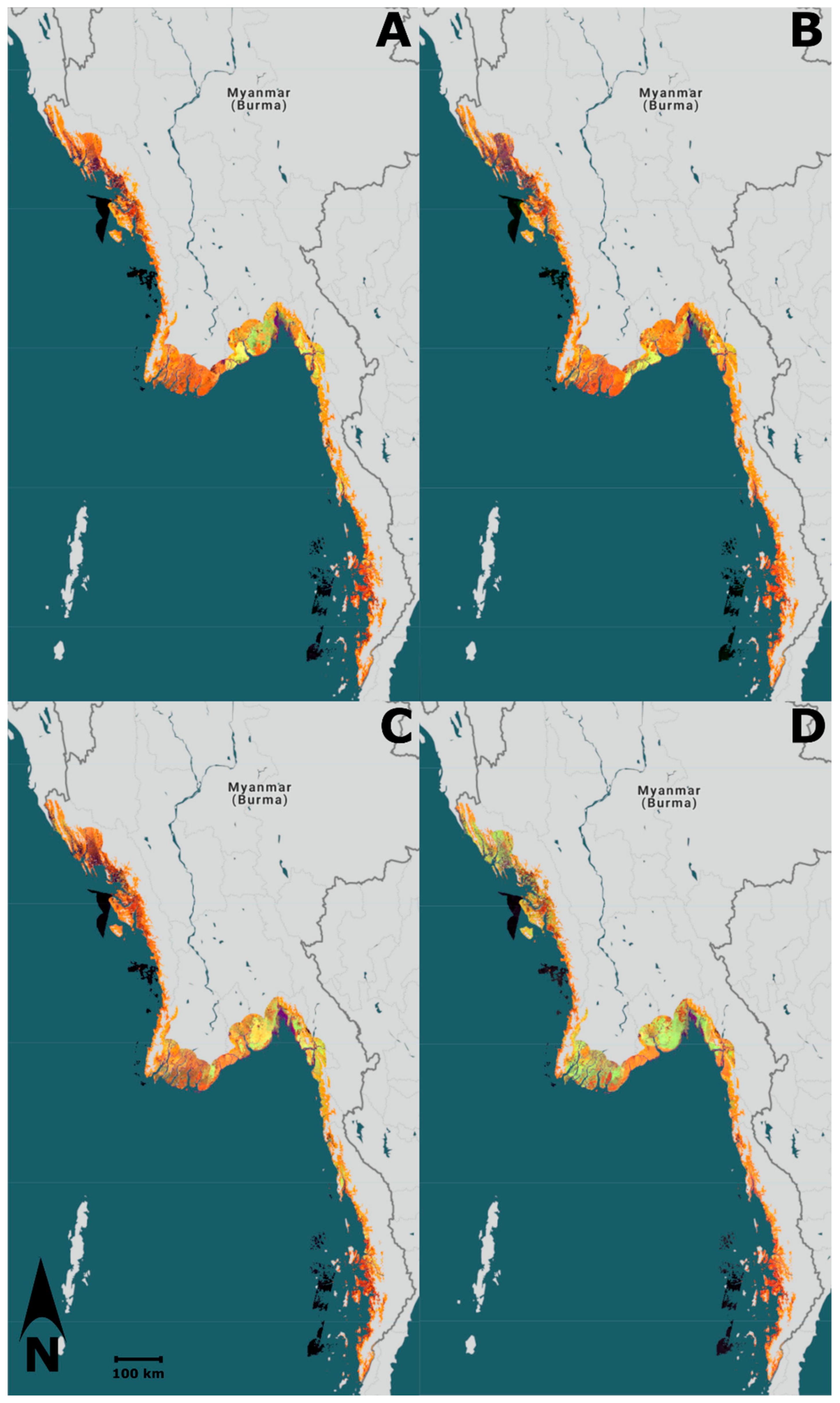
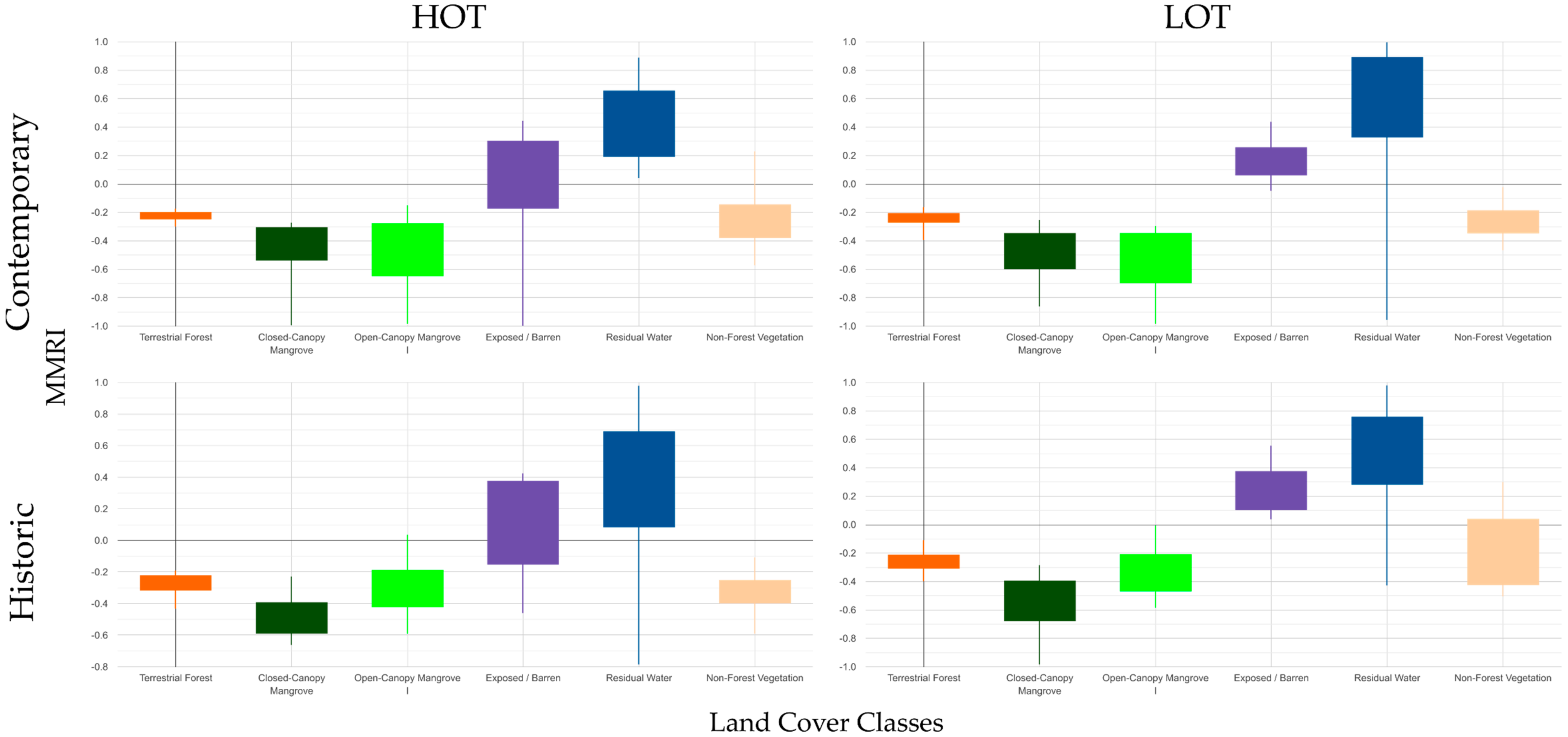
Module 1: Section 4 calculates the user selected indices from Section 1 of Module 1 (Table 3). There are a growing number of Landsat-related spectral indices available, many of which relate directly to mangroves such as the submerged mangrove recognition index (SMRI) and the modular mangrove recognition index (MMRI) [29,43]. The GEEMMM provides the user with the option to select from 14 spectral indices, of which four are mangrove-specific. The selected indices are calculated for both contemporary and historic HOT and LOT composites and added as potential classification inputs. Figure 2 compares the appearance of a typical mangrove-dominated area in Myanmar across all of the available mangrove-specific spectral indices (i.e., combined mangrove recognition index (CMRI), MMRI, SMRI, MRI) in the GEEMMM [29,43,93,98].
In Module 1: Section 5 the classification extent is further reduced through masking. In accordance with numerous mangrove mapping studies (e.g., Jones et al. [91], Thomas et al. [68], and Weber et al. [105]), the GEEMMM incorporates cloud, water, slope, and elevation masks to produce a finalized AOI. The cloud mask is generated and applied before composites are produced. The water mask is calculated for each composite using the methodology established in Xu [87], where the MNDWI layer for historic and contemporary LOT composites are generated and then a threshold is applied. Pixels with a value greater than 0.09 are considered to be water and a binary mask is produced. Depending on user selection, the water mask is finalized by either using just contemporary or combining the historic and contemporary and selecting only pixels determined to be water in both composites. This pilot study used the combined water mask. The two topographic masks are generated through user-defined thresholds or automatically determined using the 99th percentile of elevation and slope for known mangroves. The Myanmar pilot study used the known mangrove extent to generate topographic masks based on elevation values > 39 m and slope values > 16%. Noting how minor elevation is within mangrove ecosystems, the elevation threshold actually represents an approximate combined elevation + canopy height past which mangroves are not found. The generated masks are combined to create a binary, single unified final mask which is applied to all composites within the finalized ROI.
Module outputs include: (1) HOT contemporary composite, (2) LOT contemporary composite, (3) HOT historic composite, (4) LOT historic composite, (5) finalized ROI, and (6) Finalized Mask.

2.2.2. Module 2—Spectral Separability, Classifications and Accuracy Assessment

For Module 2: Section 1, user inputs address classification variables and settings. The user enters the asset path for historic and contemporary classification reference areas (CRAs) (i.e., the user-defined examples of target map classes) and identifies the unique column labels for class names and numeric codes. Next, the user identifies whether CRAs are spatio-temporally invariant (i.e., each CRA represents a class example in both contemporary and historic imagery). If the CRAs are not spatio-temporally invariant, the spectral properties of the contemporary CRAs are extracted and used to define class boundaries in the historic classification(s). For classification algorithm the single option is currently random forest [106]. The user determines how many trees are employed. The final input determines classification outputs. Users have the option to select outputs from either HOT or LOT composites for contemporary and historic inputs (i.e., four possible outputs), and/or a combined classification where HOT and LOT composites are merged to create single outputs (i.e., two more possible outputs), totaling six possible classification outputs. Zhang and Tian [93] demonstrated the utility of using combined HOT and LOT image composites as classification inputs. For the Myanmar pilot, 200 trees were selected with outputs based on combined (i.e., HOT and LOT) historic and contemporary classifications (i.e., two classifications).
In Module 2: Section 2, the user can examine correlation between potential spectral indices and the spectral separability of CRAs across all potential classification inputs. The Pearson’s correlation is calculated for each selected index to all others and these values are used to generate a correlation matrix with values ranging from −1 to 1 [107]. A value of 1 means that the potential inputs have a perfect, positive, linear correlation, and a value of −1 indicates that the indices have a perfect, negative, linear correlation. Users are encouraged to select indices that are not highly correlated indicating that they provide unique information. As a general rule, correlation coefficients with absolute values greater than 0.7 are considered moderately to strongly correlated and thus present similar information [107]. Users are advised to consider that correlation coefficients are also impacted by the amount of variability in the data, the shapes of distributions, and the presence of outliers among other factors [108].
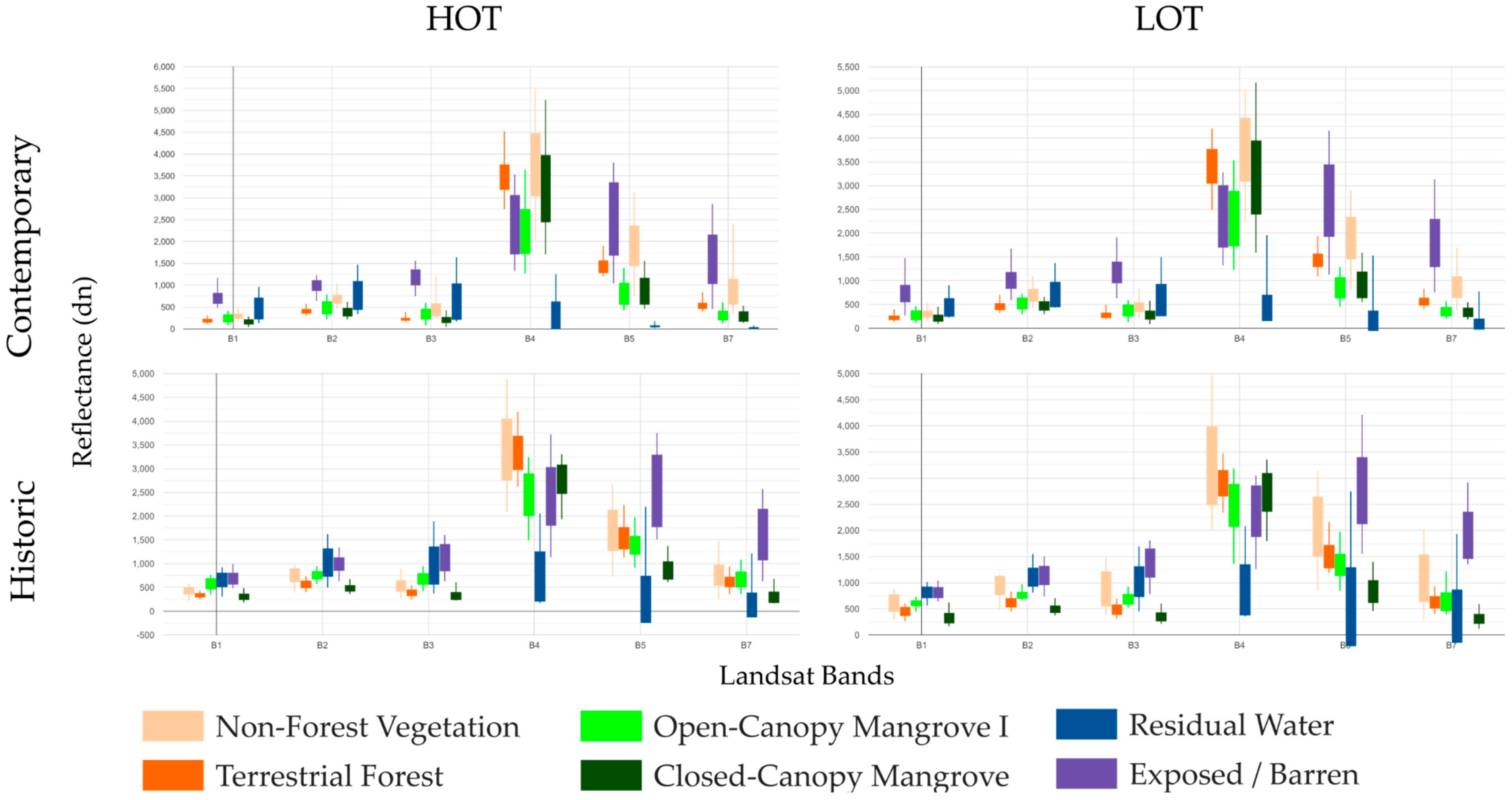
The spectral separability between target map classes as represented by CRAs is explored through the generation of three types of graphs. First, the user can view the spectral separability between each target class and each Landsat band—the user has the option to view this output for each of the four imagery composites. Box-and-whisker plots show the min, max, and inter-quartile range for each band and each map class. The second set of graphs is similar to the first, except that spectral separability is shown for individual indices across all of the target classes, showing only one index at a time. The final graph shows spectral feature space, where the x and y axes are user selected bands or indices. For the pilot study, and based on previously established precedents in Jones et al. [91], we included the visible, NIR and SWIR Landsat bands. Based on the correlation matrices and further the spectral separability they provided, the MNDWI, CMRI, MMRI, enhanced vegetation index (EVI), and Land Surface Water Index (LSWI) indices were selected as additional classification inputs.
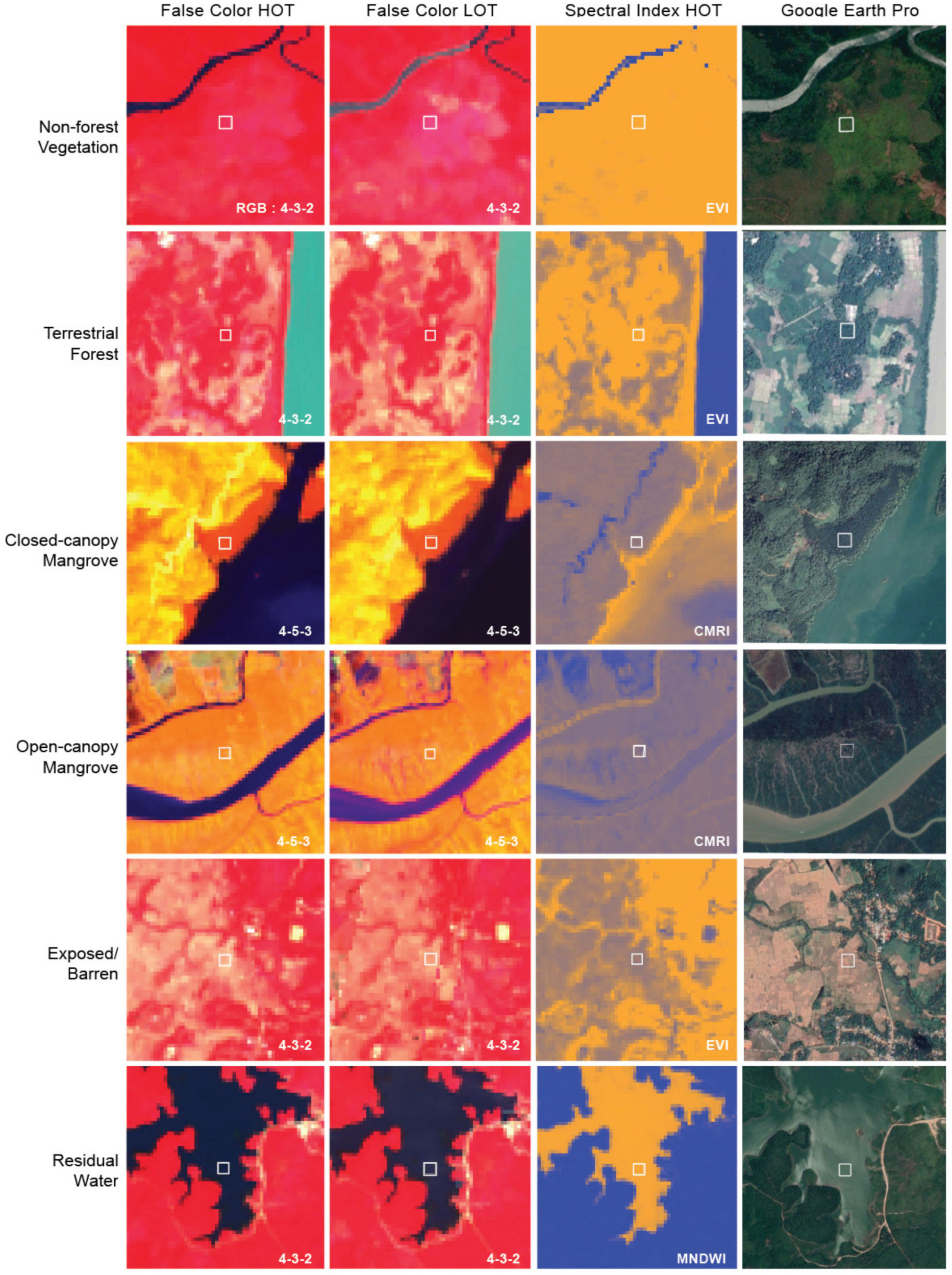
For piloting the GEEMMM in Myanmar, six classes were initially targeted, including, (1) closed-canopy mangrove, (2) open-canopy mangrove, (3) terrestrial forest, (4) non-forest vegetation, (5) exposed/barren, and (6) residual water. Table 4 provides class descriptions and an overview of how many CRAs were digitized per class. CRAs can be derived within the GEE environment or externally. For this pilot, 90 × 90 m (i.e., 3 × 3 Landsat pixels) CRAs were derived externally. To ensure that internal class variability was captured for each class and across the AOI, three sub-national AOIs were used to define CRAs (Figure 1). CRAs were derived referring to finer spatial resolution satellite imagery viewable in Google Earth Pro (Google, Mountain View, CA, USA), existing contemporary land-cover maps for Myanmar (i.e., Giri et al. [44], Saah et al. [73], and De Alban et al. [57]), and expert interpretive knowledge gained with mapping mangroves in other regions of the world. Two mangrove classes were defined to ensure that the internal variability of mangrove forests based on stature, canopy cover and density was captured. Figure 3 shows examples of all targeted classes in HOT, LOT, a key spectral index, and finer spatial resolution imagery viewable in Google Earth Pro (Google, Mountain View, CA, USA) [79].
In Module 2: Section 3: once the user confirms their final choice of classification inputs and target classes, classification—the process by which remotely sensed data is assigned land-cover classes—can occur [109,110]. There are many established algorithms for classifying Landsat data to produce maps of mangrove distribution, including classification and regression trees (CART), support vector machines (SVM), unsupervised k-means, decision trees, and maximum likelihood (ML) [28,29,42,111,112]. Many of these algorithms are available to use within the GEE environment; however, random forests—also available in GEE—is well established and used to map mangroves across the world, with distinct success within the GEE environment [27,41,43,106,113]. The inputs for random forest include an imagery data set (i.e., selected Landsat bands and spectral indices), training data (i.e., randomly selected 70% of CRAs), and a numeric parameter determining the number of ‘trees’ to be employed. For each classification the output is a single band raster with the same spatial resolution as the input data (30 m), with each pixel assigned a map value based on target classes. Following classification, the user can choose to merge map classes—this is particularly advantageous in scenarios where initial map classes were used to capture variability, but for which confidence in class boundaries may be lacking. For example, in the Myanmar pilot, we merged the two mangrove classes (i.e., closed- and open-canopy) post-classification. This ensured capturing mangrove variability while not having to draw a distinct boundary between these potentially overlapping classes in the final map.
Classification accuracy—defined as “a comparison of the derived product to ground condition”—is not reported in numerous studies involving mangrove mapping [114,115]. Following classification and optional class merging, in Module 2: Section 3, the GEEMMM automatically produces resubstitution and error matrices for all output classifications [116]. The resubstitution matrices determine end land-cover class for the CRAs used for training the classifier. The error matrices use 30% of CRAs held back from classification to independently evaluate map accuracies. The overall accuracy is reported using the error matrix ‘accuracy’ tool, found within the GEE library. Overall accuracy is printed below both the error and resubstitution matrices. By reviewing the error matrices and visually inspecting the output maps the user may wish to collapse/further collapse classes (e.g., if two classes are very confused). If the user combines classes, they can opt to re-calculate accuracy, re-generating resubstitution and error matrices. The final step for all users to exporting the classification maps to their assets. Module 2 outputs include, (1) correlation and spectral separability graphs, (2) classified maps, and (3) accuracy assessments.

2.2.3. Module 3—Dynamics and QAA

In Module 3: Section 1, the user indicates which classification(s) will be used to calculate dynamics and/or assess optional QAA. If desired, the user can further clip classifications to a country’s boundary—if pertinent—using the GEE Large Country Boundary Polygons, or by uploading an external dataset. For the Myanmar pilot we further clipped using a uniquely uploaded boundary (GADM) and exclusive economic zone (EEZ) from Marine Regions (v10 World EEZ,) [117]. For the QAA, the user enters CRA information (e.g., asset path, class names, and unique class numbers).
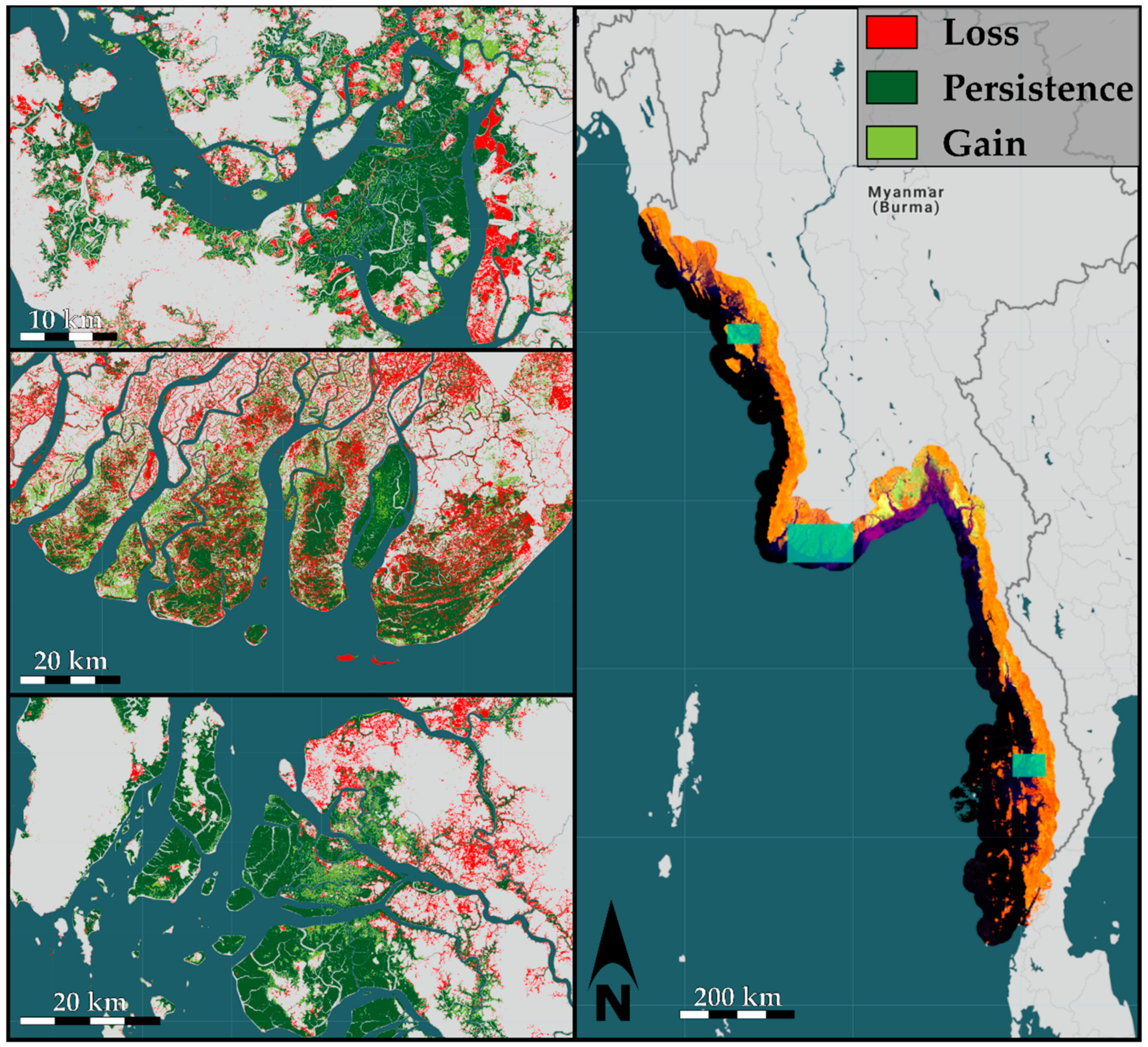
In Module 3: Section 2, multi-date outputs are used to quantify dynamics. This is foundational to understanding long-term trends and the effectiveness of conservation efforts. The user selects which map class they would like to view, and loss, persistence, and gain (i.e., LPG) are calculated. The automatically produced, self-masked layers are added to the GEE-GUI map interface. The resulting area for each dynamic assessment is printed to the console, expressed in hectares. Building on the inventory, description, acquisition and comparison of existing datasets, the dynamics resulting from this GEEMMM pilot were also compared to published values.
Module 3: Section 3—building on the previously referenced methods detailed in Gandhi and Jones [19]—facilitates an optional QAA. For this GEEMMM QAA, an interactive map is divided into three linked maps (Figure 1). In each map, two sets of grids are automatically generated, (1) 100 km by 100 km grids, and (2) within each of those cells, sub-divided 10 km by 10 km grids. The 100 km × 100 km grid cells are randomly selected, retaining 50% of the grid cells that intersect the ROI. In slight contrast to the baseline QAA described in Section 2.1.4, for the QAA tool in the GEEMMM, within each selected grid cell, 20% of the sub-grid cells are selected. The tool works by cycling through the sub grid cells, and giving the user the option to view simultaneously on linked maps showing Landsat composites where the date can be changed at the user’s preference, the classifications produced in Module 2, and the imagery used for the classifications generated in Module 1. The user then has the ability to record in the GUI whether each map class is under-, well-, or over-represented, and record ‘free comments’ for each sub-cell.
Module 3 outputs include: automatically generated LPG as raster and—if performed—QAA grid (for viewing outside of GEE). The user also has the option to export the QAA table (containing the under, over, and well representation statistics, and the free comments) as a CSV (i.e., comma separated values) file at any point during the QAA.

3. Results and Discussion

3.1. Myanmar—Comparison of Existing Datasets

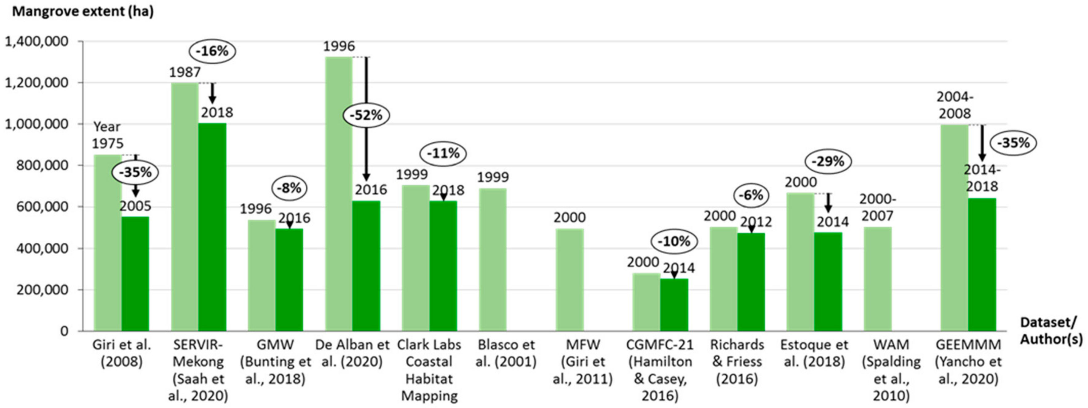
Table 5 provides a comparison of all single- and multi-date datasets based on dataset/authors, year, extent (ha), dynamics (ha and %), whether discrete or continuous, mapped classes, accuracy, and known limitations. Figure 4 provides a comparison of all distributions across time across all datasets. Results show that Myanmar’s mangrove distribution ranged from 851,452–1,323,300 ha circa 1975–1987 (i.e., historic) to 475,637–1,002,098 ha circa 2014–2018 (i.e., contemporary). Of the 11 existing studies, only five provided quantitative accuracy assessments, with overall accuracies ranging from 76% (i.e., Saah et al. [73]) to 97% (i.e., Estoque et al. [56]), mangrove producer’s accuracies ranging from 75% (i.e., De Alban et al. [57]) to 93.1% (i.e., also De Alban et al. [57]), and mangrove user’s accuracies ranging from 92.3% (i.e., De Alban et al. [57]) to 98.1% (i.e., Clark Labs [75]). Of the existing studies, eight provided dynamics, including a loss of 300,091 ha/35.2% from 1975–2005 (Giri et al. [70]), 195,227 ha/16.3% from 1987–2018 (Saah et al. [73]), 43,208 ha/8.0% from 1996–2016 (Bunting et al. [74]), 694,600 ha/52.5% from 1996–2016 (De Alban et al. [57]), 76,465 ha/10.9% from 1999–2018 (Clark Labs [75]), 27,064 ha/9.7% from 2000–2014 (Hamilton and Casey [78]), 27,770 ha/5.5% from 2000–2012 (Richards and Friess [47]), and 191,122 ha/28.7% from 2000–2014 (Estoque et al. [56]). Two reported specifically on sub-national loss hotspots (i.e., De Alban et al. [57] and Estoque et al. [56]). According to De Alban et al. [57], Bago, Mon, Yangon—the three states immediately to the east of the Ayeyarwady delta—suffered greatest proportionate loss from 1996–2016 totaling more than 80% of their extents. In terms of absolute loss, from 2000–2014, Estoque et al. [56] reported Rakhine as the state with the greatest loss (75,494 ha/39.5% of Myanmar’s total loss), followed by Ayeyarwady experiencing 69,431 ha/36.3% of Myanmar’s total loss.
Direct comparisons of existing datasets are challenging due to differences in temporal coverage, methodologies, and imagery sources. Although most studies use optical imagery (typically medium-resolution Landsat), some of the more recent studies combine optical with radar imagery (e.g., Bunting et al. [74]; De Alban et al. [57]). Several different mapping techniques are employed, while two of the datasets (Hamilton and Casey [78]; Richards and Friess [47]) calculate and present continuous measures of mangrove canopy cover, rather than discrete (i.e., presence vs no presence). Interpreting continuous datasets for areal mangrove extent is problematic as pixels containing just 0.01% canopy cover are included as mangrove falling well below commonly used minimum definitions mangrove forest (e.g., 30%) [18,78,91].
Of the five datasets reporting, all achieve overall accuracies of >75%, with four >85% [56,57,74,75]. QAAs further identified Clark Labs [75] as mapping mangroves in Myanmar most consistently. Mangroves were under-represented in the remaining five datasets assessed, particularly in Giri et al. [70] and Saah et al. [73], but also in Bunting et al. [74] (Table 6).
Existing studies clearly establish that Myanmar has experienced consequential mangrove loss; however, baseline distributions and dynamics (when available) are highly variable. These discrepancies are likely attributed to the differences highlighted in Table 5. In addition, the definitions for mangroves and surrounding land-cover classes and the actual examples used for classification (i.e., CRAs) likely further account for differences. Only with agreed upon conventions for defining mangroves and providing examples as CRAs can cross-study comparisons become standardized and optimized. Falling short of this, discrepancies will remain common.

3.2. Results of the Google Earth Engine Mangrove Mapping Methodology (GEEMMM)

3.2.1. Module 1—Defining AOI and Compositing Imagery

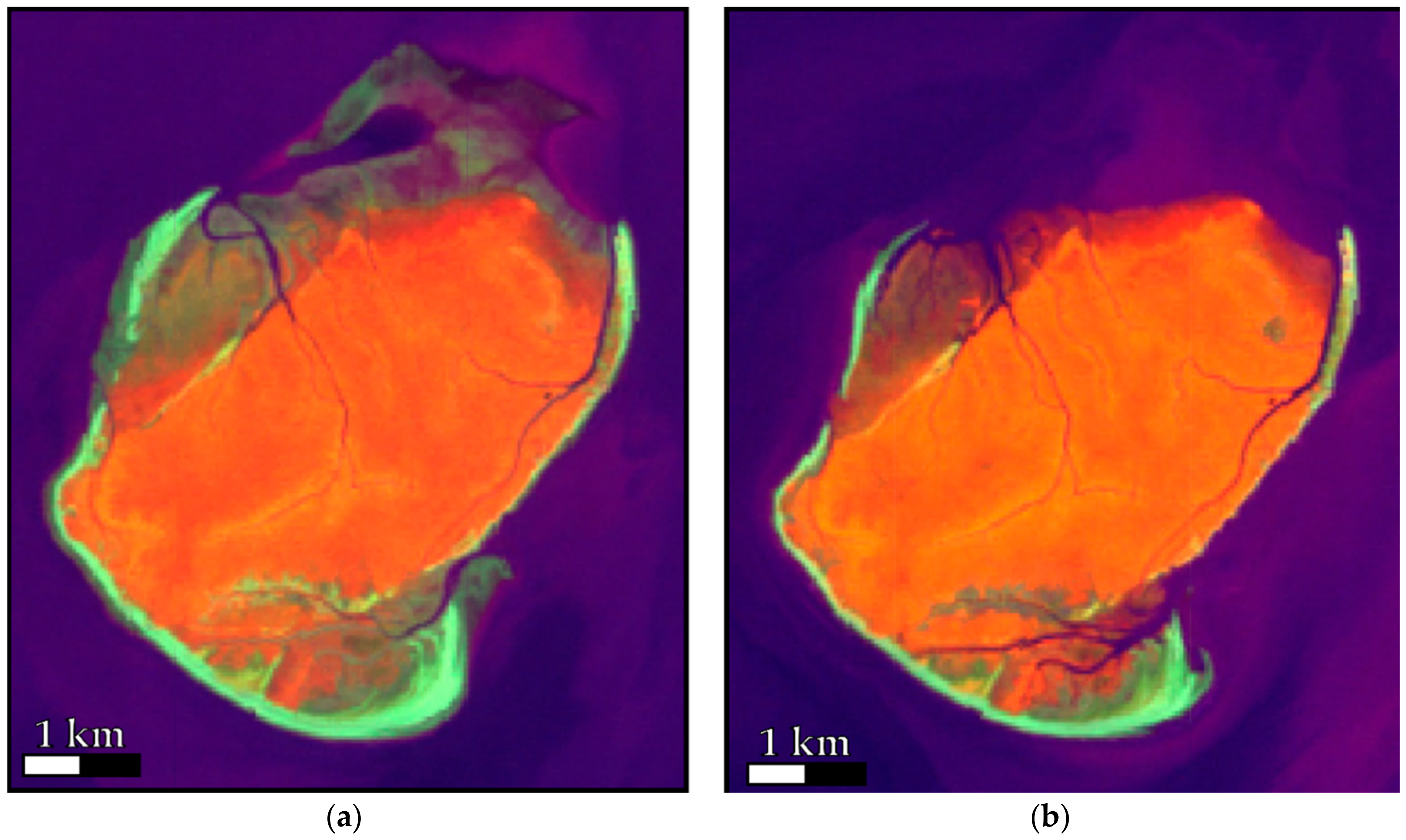
As confirmed through qualitative yet systematic spot-checks, the imagery generated from the Myanmar pilot reflects the selected inputs well—both historic and contemporary composites are mostly cloud- and artifact-free, and clearly represent distinct HOT and LOT conditions (Figure 5). Figure 6 shows a national overview of the AOI including contemporary and historic HOT and LOT composites. The challenges that have been identified can be attributed to the extent of the study area and trying to capture a long, complex coastline in a series of contiguous composites. The most notable challenge relates to seasonal variability observed primarily in areas where large clouds were masked out of one image and the pixels selected to fill captured seasonally different land-cover conditions. Notably, this issue was almost entirely associated with areas which undergo significant changes throughout the year, i.e., agricultural mosaics and non-forest vegetation. Even within the defined seasonal window, variability was observed. Users are advised to select meaningful seasonal windows that restrict such variability while still offering enough imagery to make optimal composites—this is constrained by the size of the AOI.

3.2.2. Module 2—Spectral Separability, Classifications and Accuracy Assessment

Based on correlation analysis of all available spectral indices, five (i.e., MNDWI, CMRI, MMRI, EVI, and LSWI) stood out as not correlated (Appendix A) and were selected as classification inputs. Using the spectral separability tools, all target classes as represented by CRAs were assessed across all non-thermal (red, green, blue, NIR, SWIR1, and SWIR2) Landsat bands (Figure 7), and each selected index was further evaluated to confirm that it provided additional separation for one or more classes (e.g., MMRI: Figure 8). Results indicate that bands SWIR1 and SWIR2 were particularly helpful in separating non-forest vegetation. Non-forest vegetation was most confused with other vegetation classes in the visible spectrum and MNDWI. For terrestrial forest, NIR, MNDWI, and MMRI provided separability. In particular, MNDWI provided good separation from mangroves; whereas within the visible spectrum and CMRI the most confusion was noted, particularly with other vegetation classes. Closed-canopy mangrove was best distinguished by LSWI, MMRI, and to a limited extent bands SWIR1 and SWIR2. In contrast, open-canopy mangrove was best distinguished by CMRI, MNDWI, NIR, SWIR1, and SWIR2. While there are meaningful and distinct differences between the two canopy-based mangrove classes, there is spectral overlap—this speaks to the advantage of capturing the variability within mangrove forests while subsequently merging into a single class post-classification. Field work is required to confidently define the boundaries between these sub-mangrove types to make them final map classes—following classification and prior to validation, mangroves were merged into a single class (i.e., mangrove). Taken together, the combined mangrove class exhibited some confusion with terrestrial forest and non-forest vegetation classes in EVI, the visible bands, and SWIR1 and SWIR2. The exposed/barren class had the most separability in indices CMRI, MMRI, and LSWI, and the most confusion with non-forest vegetation and terrestrial forest notably in MNDWI and residual water in the visible bands. Residual water was easily distinguished with MNDWI, and the non-visible bands, but was confused with exposed/barren in the visible bands, non-forest vegetation within CMRI, and all classes within EVI.
For both historic and contemporary classifications, resubstitution accuracies were 100%, indicating all training data was assigned to the correct land-cover class. Based on accuracy assessments using independent validation data, overall accuracies for historic and contemporary classifications were 97.0 and 98.5%, respectively (Table 7). For the contemporary classification, there was slight confusion between terrestrial forest and mangroves. Additionally, there was a small amount of two-way confusion between non-forest vegetation and terrestrial forest. The greatest source of error for the historic classification was the non-forest vegetation class, which was at-times confused with mangroves and the exposed/barren class.

3.2.3. Module 3—Dynamics and QAA

Classification results indicate that circa 2004–2008, Myanmar contained 995,412 ha of mangroves. In contrast, by 2014–2018, Myanmar contained 642,659 ha of mangroves. These results suggest that from 2004–2008 to 2014–2018 there was 551,570.99 ha of loss and 198,818.42 ha of gain (i.e., net loss 352,752.57 ha or 35.4%) (Figure 4 and Figure 9, Table 5). As compared to Estoque et al. [56] and Giri et al. [70], estimated rates of loss are within reported trends and ranges; however, other studies reported lower rates of loss often coinciding with lower total estimates of mangrove cover (i.e., Bunting et al. [74]; Hamilton and Casey [78]; Richards and Friess [47]; Estoque et al. [56]). Figure 9 shows LPG from GEEMMM results within the loss hotspots identified through existing literature (i.e., Figure 1).
While there was a substantial net loss based on GEEMMM results, the reported gain seems relatively high. Portions of this likely reflect actual natural processes and increases in mangrove extent; however, the overall gain estimate is likely an overestimation. Exaggerated gain likely reflects the desk-based process of deriving CRAs. Clearly any classification is only as good as the examples used to calibrate the algorithm, and a limitation of this pilot was no direct access to field observations or ground truth, and constrained access to historical high spatial resolution satellite imagery. Disproportionate mangrove gain therefore likely reflects an underrepresentation of lower stature, less dense mangroves in the historic classification, which in turn exaggerates the amount of supposed gain (i.e., many of these areas were likely actually mangroves in both dates). Extensive field work and ground verification is required to confirm.
The GEEMMM QAA was conducted for the contemporary map, then repeated for the historic map. As part of the contemporary QAA, spot-checks were conducted over 108 sub-grid cells across Myanmar (Figure 1). The mangrove class was generally well-represented; however, at-times under-represented in favor of classes depicting portions of areas in the variable agricultural mosaic, i.e., non-forest vegetation, and exposed/barren. In both the contemporary, and less so the historic map, the agricultural mosaic was depicted as a patchwork of these two classes, on a pixel-by-pixel basis, given the inherent variability within the seasonal window. This resulted in some confusion between the two classes, and to some extent an under-representation of mangroves. In the contemporary map, sparser mangroves at the ecosystem periphery were at-times misclassified as non-forest vegetation, thereby under-representing mangrove and over-representing non-forest vegetation. Terrestrial forest was also at-times over-represented, occasionally at the expense of actual mangrove areas. Overall, the contemporary classification appeared to best represent Myanmar’s south (i.e., the Tanintharyi coastline). The historic QAA, while not quite as comprehensive as the contemporary QAA (mainly due to the absence of historic imagery in GEE), found the mangrove class to be generally well-represented, though at-times over-represented at the expense of classes depicting the agricultural mosaic—an inverse to the contemporary map. Some portions of the agricultural mosaic were also found to be misclassified as terrestrial forest. As with the contemporary map, Myanmar’s southern Tanintharyi coastline seemed best represented. Notably, most existing studies did not provide standard quantitative accuracy assessments, and no existing studies went beyond these and further qualitatively assessed resulting maps. While quantitative accuracy assessments should be a standard part of reporting, QAAs also help further assess resulting maps and identify areas for improvement. As such, the GEEMMM goes beyond standard accuracy—for which GEEMMM results were very high—and allows users to more closely examine actual distributions and subsequently dynamics.

3.2.4. Dissemination and Improvement

The code is available in a GitHub repository (see Supplementary Materials Section), with a GNU GPLv3 license permitting free use, modification, and sharing, provided that the source is disclosed and not used for commercial purposes. The code runs based on provided links, or is copied-and-pasted into GEE, which remains available for free non-profit and educational use. The tool itself continues to be adjusted and updated, as the GEE library evolves and as new mangrove remote sensing techniques become available.
While the tool performs well there are always potential improvements. Notably, CRAs are a key input for the workflow, and highly influence the outcome of the classifications. Future applications of the GEEMMM would benefit from direct access to field-based ground truth when deriving CRAs, particularly when it comes to confidently using mangrove sub-types as final map classes. While the need for and merit of isolating tidal conditions is proven, which tidal conditions are best requires further exploration—we used combined HOT and LOT in this pilot, whereas HOT or LOT on its own could also be employed. Furthermore, the choice of tidal condition depends on the intended application. For example, mangrove carbon projects may favor using HOT composites on their own for more conservative estimates of mangrove extent and change.
While going beyond standard accuracy metrics, the QAA is a somewhat complex component requiring significant user interaction; however, it too will evolve as the GEEMMM is further tested with other settings and applied to other AOIs. GEE itself also has notable limitations: the AOI can be as large or as small as the user requires but GEE has computational limits. Google shares its cloud processing among all GEE users, which means that if the task requested to process is too large (e.g., a long complex coastline, with collections containing hundreds of images) the user’s allocated capacity may be exceeded and error(s) returned. Additionally, the functioning of this tool requires a relatively stable and reasonably strong internet connection, especially to view images and products within the GUI. If internet connectivity is limited, there may be latency issues loading data or even time-out errors. One of the benefits of working within the GEE environment however is that once a data product export has begun it will be completed on Google’s server side. This means that internet access can be interrupted while using the tool, and it will continue to run. It was this feature of GEE, the server-side image/vector data exporting that drove the current configuration of three modules, where intermediate data products are exported to the user’s assets, effectively saving their progress through the tool.
The GEEMMM is currently designed around the use of Landsat data—this was a conscious choice based around data availability. Sentinel imagery—which is also available through GEE—offers an increased revisit time (i.e., higher temporal resolution) and finer spatial resolution; however, it remains limited by a 2015-present temporal window. In contrast, the Landsat archive in GEE offers >35 years of imagery which facilitates more historically meaningful and robust dynamics assessments while also providing enough imagery to draw from multiple years to produce composites within preferred seasonal windows. Given the added benefits—especially once the archive spans 10+ years—future versions of the GEEMMM should also offer the choice of Sentinel imagery to users as an option.

4. Conclusions

We present a new tool—the GEEMMM—for mapping and monitoring mangrove ecosystems. By leveraging GEE, this new tool circumvents many traditional barriers to conventional methods. In addition, it presents an internal, image-based approach for tidal calibration. The GEEMMM—including the well commented source code—is available online and is ready to be used by practitioners anywhere mangrove ecosystems exist; please see information in Supplementary Material Section on how to access the GEEMMM.
While operational, the GEEMMM is not without its limitations: the larger the area the more complex the mapping task, particularly when it comes to creating optimal imagery composites within defined seasonal windows. In addition, the upper limits of GEE and internet connectivity present a challenge in terms of the time associated with and reliability of running the GEEMMM; however, when compared to the conventional processing times associated with standalone workstations it remains much faster, and once a part of the GEEMMM starts running it will continue to run even if the internet connection is lost. In any application, the resulting maps and dynamics assessments will only ever be as good as the examples of target map classes provided. Coastal managers will normally have such information available to them and GEEMMM provides them with a framework through which to capitalizes on this local knowledge, rather than relying on external datasets, which allow little to no customization, to map and monitor their mangroves.
The GEEMMM makes a significant and ready-to-go contribution toward accessible mangrove mapping and monitoring. It also remains a living tool wherein non-profit users are encouraged by the authors to make useful suggestions for modifications or additions, or modify the tool directly themselves to meet their own customized needs. While piloting the GEEMMM for Myanmar is an important first step, additional applications and tests are required, particularly for smaller areas of interest, wherein the GEEMMM can help fill a critical sub-national mapping gap. The authors welcome the opportunity to receive feedback from and work with users to more comprehensively assess the tool and gauge areas for improvement. A series of in-person and online instructional materials will go a long way toward ensuring the maximum and optimal utility of the GEEMMM. This first iteration of the GEEMMM further sets the stage for a comparatively more automated and even more accessible version to be deployable completely on mobile devices.

Supplementary Materials

The GEEMMM tool is freely available within the GitHub repository: https://github.com/Blue-Ventures-Conservation/GEEMMM.

Author Contributions

The GEEMMM was conceived of by, T.G.J., S.R.G., L.G., C.F., and J.M.M.Y. Contributions to the methodology were made by T.G.J., S.R.G., and C.F., with J.M.M.Y. developing the key tidal detection methods. J.M.M.Y. wrote all of the code in GEE for the GEEMMM tool, with the work reviewed by C.F. The results of this paper were validated by J.M.M.Y., T.G.J., S.R.G., C.F., and A.L. Formal analysis was performed by J.M.M.Y., T.G.J., and S.R.G., using the analysis tools developed by J.M.M.Y. Investigation for this work was conducted by J.M.M.Y., T.G.J., S.R.G., C.F., and A.L., J.M.M.Y. performed all of the data curation for this paper. The original manuscript writing was conducted by T.G.J. and J.M.M.Y.; with T.G.J. writing the introduction, discussion points, and conclusion and J.M.M.Y. writing the bulk of the methods and results. All authors, T.G.J., J.M.M.Y., S.R.G., C.F., A.L., and, L.G. were involved in writing—review and editing. Visualizations were generated by J.M.M.Y., A.L., and S.R.G. The project was administrated and supervised by T.G.J. and L.G. All authors have read and agreed to the published version of the manuscript.

Funding

This research was funded by Blue Ventures Conservation, with support from the UK Government’s International Climate Fund, part of the UK commitment to developing countries to help them address the challenges presented by climate change and benefit from the opportunities.

Acknowledgments

We thank the following authors of studies referenced in this paper: Ake Rosenqvist, of solo Earth Observation (soloEO), for provision of and support regarding GMW data; J. Ronald Eastman and James Toledano, of Clark Labs, for guidance regarding the Clark Labs Aquaculture dataset; Chandra Giri, of United States Environmental Protection Agency, for provision of data and associated guidance; Edward L. Webb, of National University Singapore, for data provision and guidance; and Ate Poortinga, of Spatial Informatics Group, for provision of and guidance regarding SERVIR-Mekong data.

Conflicts of Interest

The authors declare no conflict of interest.

Appendix A

Table A1. Correlation matrices for the calculated spectral indices for both HOT and LOT historic and contemporary imagery extracted from the CRAs.
Contemporary HOT Index Band Correlation
SRNDVINDWIMNDWICMRIMMRISAVIOSAVIEVIMRISMRILSWINDTIEBBI
SR10.654−0.61−0.420.256−0.460.6540.6540.130.018−0.140.4980.719−0.71
NDVI0.6541−0.98−0.850.177−0.70.9990.9990.203−0.11−0.380.1630.755−0.76
NDWI−0.61−0.9810.9070.0050.679−0.98−0.98−0.180.1180.392−0.06−0.690.698
MNDWI−0.42−0.850.90710.2220.475−0.85−0.85−0.140.2220.3420.328−0.430.448
CMRI 0.2560.1770.0050.2221−0.180.1770.1770.1408.709 *0.5620.407−0.4
MMRI −0.46−0.70.6790.475−0.181−0.7−0.7−0.08−0.040.154−0.31−0.720.617
SAVI 0.6540.999−0.98−0.850.177−0.710.9990.203−0.11−0.380.1630.755−0.76
OSAVI0.6540.999−0.98−0.850.177−0.70.99910.203−0.11−0.380.1630.755−0.76
EVI0.130.203−0.18−0.140.14−0.080.2030.2031−0.01−0.090.0320.145−0.15
MRI0.018−0.110.1180.2220−0.04−0.11−0.11−0.0110.0330.2270.0670.085
SMRI−0.14−0.380.3920.3428.709 *0.154−0.38−0.38−0.090.03310.028−0.270.175
LSWI0.4980.163−0.060.3280.562−0.310.1630.1630.0320.2270.02810.566−0.6
NDTI0.7190.755−0.69−0.430.407−0.720.7550.7550.1450.067−0.270.5661−0.79
EBBI−0.71−0.760.6980.448−0.40.617−0.76−0.76−0.150.0850.175−0.6−0.791
*—Denotes an error output from the GEE servers for the index correlations.
Contemporary LOT Index Band Correlation
SRNDVINDWIMNDWICMRIMMRISAVIOSAVIEVIMRISMRILSWINDTIEBBI
SR10.718−0.67−0.440.286−0.470.7180.7180.1580.054−0.140.5090.717−0.76
NDVI0.7181−0.97−0.790.234−0.780.9990.9990.223−0.1−0.250.2670.75−0.79
NDWI−0.67−0.9710.871−0.020.774−0.97−0.97−0.230.1190.236−0.14−0.670.714
MNDWI−0.44−0.790.87110.270.492−0.79−0.79−0.220.2510.2210.337−0.30.374
CMRI0.2860.234−0.020.271−0.130.2340.234−0.030.033−0.10.6120.459−0.46
MMRI−0.47−0.780.7740.492−0.131−0.78−0.78−0.21−0.040.137−0.37−0.690.65
SAVI0.7180.999−0.97−0.790.234−0.7810.9990.223−0.1−0.250.2670.75−0.79
OSAVI0.7180.999−0.97−0.790.234−0.780.99910.223−0.1−0.250.2670.75−0.79
EVI0.1580.223−0.23−0.22−0.03−0.210.2230.2231−0.02−0.040.0060.126−0.17
MRI0.054−0.10.1190.2510.033−0.04−0.1−0.1−0.0210.0330.2530.081−0.02
SMRI−0.14−0.250.2360.221−0.10.137−0.25−0.25−0.040.0331−0.01−0.140.134
LSWI0.5090.267−0.140.3370.612−0.370.2670.2670.0060.253−0.0110.716−0.67
NDTI0.7170.75−0.67−0.30.459−0.690.750.750.1260.081−0.140.7161−0.89
EBBI 0.76−0.790.7140.374−0.460.65−0.79−0.79−0.17−0.020.134−0.67−0.891
Historic HOT Index Band Correlation
SRNDVINDWIMNDWICMRIMMRISAVIOSAVIEVIMRISMRILSWINDTIEBBI
SR10.844−0.78−0.560.603−0.740.8440.8440.406−0.17−0.260.1230.373−0.83
NDVI 0.8441−0.98−0.830.418−0.820.9990.9990.38−0.25−0.45−0.260.248−0.69
NDWI −0.78−0.9810.894−0.260.773−0.98−0.98−0.340.2320.490.38−0.20.595
MNDWI−0.56−0.830.89410.0270.618−0.83−0.83−0.260.2390.4350.718−0.060.244
CMRI0.6030.418−0.260.0271−0.540.4180.4180.341−0.210.030.560.341−0.77
MMRI−0.74−0.820.7730.618−0.541−0.82−0.82−0.450.1840.2790.031−0.330.719
SAVI0.8440.999−0.98−0.830.418−0.8210.9990.38−0.25−0.45−0.260.248−0.69
OSAVI0.8440.999−0.98−0.830.418−0.820.99910.38−0.25−0.45−0.260.248−0.69
EVI0.4060.38−0.34−0.260.341−0.450.380.381−0.09−0.020.0640.151−0.38
MRI−0.17−0.250.2320.239−0.210.184−0.25−0.25−0.091−0.160.104−0.020.231
SMRI−0.26−0.450.490.4350.030.279−0.45−0.45−0.02−0.1610.2670.0890.16
LSWI0.123−0.260.380.7180.560.031−0.26−0.260.0640.1040.26710.23−0.45
NDTI0.3730.248−0.2−0.060.341−0.330.2480.2480.151−0.020.0890.231−0.38
EBBI−0.83−0.690.5950.244−0.770.719−0.69−0.69−0.380.2310.16−0.45−0.381
Historic LOT Index Band Correlation
SRNDVINDWIMNDWICMRIMMRISAVIOSAVIEVIMRISMRILSWINDTIEBBI
SR10.852−0.77−0.420.529−0.770.8520.8520.1350.158−0.30.4120.714−0.82
NDVI0.8521−0.97−0.740.325−0.860.9990.9990.1830.037−0.390.0840.705−0.69
NDWI−0.77−0.9710.842−0.110.824−0.97−0.97−0.180.0560.3980.072−0.630.574
MNDWI−0.42−0.740.84210.280.539−0.74−0.74−0.140.270.240.586−0.280.086
CMRI0.5290.325−0.110.281−0.380.3250.3250.0410.429−0.080.7240.485−0.71
MMRI−0.77−0.860.8240.539−0.381−0.86−0.86−0.14−0.150.341−0.25−0.670.728
SAVI0.8520.999−0.97−0.740.325−0.8610.9990.1830.037−0.390.0840.705−0.69
OSAVI0.8520.999−0.97−0.740.325−0.860.99910.1830.037−0.390.0840.705−0.69
EVI0.1350.183−0.18−0.140.041−0.140.1830.18310.004−0.010.0080−0.11
MRI0.1580.0370.0560.270.429−0.150.0370.0370.0041−0.160.4140.167−0.32
SMRI−0.3−0.390.3980.24−0.080.341−0.39−0.39−0.01−0.161−0.11−0.250.322
LSWI0.4120.0840.0720.5860.724−0.250.0840.0840.0080.414−0.1110.405−0.71
NDTI0.7140.705−0.63−0.280.485−0.670.7050.70500.167−0.250.4051−0.72
EBBI−0.82−0.690.5740.086−0.710.728−0.69−0.69−0.11−0.320.322−0.71−0.721

References

  1. Saenger, P. Mangrove Ecology, Silviculture and Conservation; Springer Science & Business Media: Berlin, Germany, 2002; Volume 3, ISBN 9789048160501. [Google Scholar]
  2. Food and Agriculture Organization of the United Nations; Forestry Department (Rome). Global Forest Resources Assessment 2000: Main Report; Food and Agriculture Organization of the United Nations: Rome, Italy, 2001. [Google Scholar]
  3. Xia, Q.; Qin, C.Z.; Li, H.; Huang, C.; Su, F.Z.; Jia, M.M. Evaluation of submerged mangrove recognition index using multi-tidal remote sensing data. Ecol. Indic. 2020, 113. [Google Scholar] [CrossRef]
  4. Lugo, A.E. Mangrove Ecosystems: Successional or Steady State? Biotropica 1980, 12, 65–72. [Google Scholar] [CrossRef]
  5. Spalding, M.; Kainuma, M.; Collins, L. World Atlas of Mangroves; Earthscan: New York, NY, USA, 2010; ISBN 978-1-84407-657-4. [Google Scholar]
  6. Duke, N.; Nagelkerken, I.; Agardy, T.; Wells, S.; van Lavieren, H. The Importance of Mangroves to People: A Call to Action; van Bochove, J.-W., Sullivan, E., Nakamura, T., Eds.; United Nations Environment Programme World Conservation Monitoring Centre: Cambridge, UK, 2014; ISBN 9789280733976. [Google Scholar]
  7. Scales, I.R.; Friess, D.A.; Glass, L.; Ravaoarinorotsihoarana, L. Rural livelihoods and mangrove degradation in south-west Madagascar: Lime production as an emerging threat. Oryx 2018, 52, 641–645. [Google Scholar] [CrossRef] [Green Version]
  8. Blue Ventures Conservation. Value Chain Analysis: The wild capture mud crab fishery of Madagascar’s Menabe region. Available online: https://blueventures.org/publication/value-chain-analysis-the-wild-capture-mud-crab-fishery-of-madagascars-menabe-region/ (accessed on 1 October 2020).
  9. Aye, W.N.; Wen, Y.; Marin, K.; Thapa, S.; Tun, A.W. Contribution of mangrove forest to the livelihood of local communities in Ayeyarwaddy Region, Myanmar. Forests 2019, 10, 414. [Google Scholar] [CrossRef] [Green Version]
  10. Nagelkerken, I.; Blaber, S.J.M.; Bouillon, S.; Green, P.; Haywood, M.; Kirton, L.G.; Meynecke, J.O.; Pawlik, J.; Penrose, H.M.; Sasekumar, A.; et al. The habitat function of mangroves for terrestrial and marine fauna: A review. Aquat. Bot. 2008, 89, 155–185. [Google Scholar] [CrossRef] [Green Version]
  11. Gopal, B.; Chauhan, M. Biodiversity and its conservation in the Sundarban mangrove ecosystem. Aquat. Sci. 2006, 68, 338–354. [Google Scholar] [CrossRef]
  12. Gardner, C.J. Use of Mangroves by Lemurs. Int. J. Primatol. 2016, 37, 317–332. [Google Scholar] [CrossRef] [Green Version]
  13. Alongi, D.M. Carbon cycling and storage in mangrove forests. Annu. Rev. Mar. Sci. 2014, 6, 195–219. [Google Scholar] [CrossRef]
  14. Donato, D.C.; Kauffman, J.B.; Murdiyarso, D.; Kurnianto, S.; Stidham, M.; Kanninen, M. Mangroves among the most carbon-rich forests in the tropics. Nat. Geosci. 2011, 4, 293–297. [Google Scholar] [CrossRef]
  15. Sanderman, J.; Hengl, T.; Fiske, G.; Solvik, K.; Adame, M.F.; Benson, L.; Bukoski, J.J.; Carnell, P.; Cifuentes-Jara, M.; Donato, D.; et al. A global map of mangrove forest soil carbon at 30 m spatial resolution. Environ. Res. Lett. 2018, 13. [Google Scholar] [CrossRef]
  16. Rakotomahazo, C.; Ravaoarinorotsihoarana, L.A.; Randrianandrasaziky, D.; Glass, L.; Gough, C.; Boleslas Todinanahary, G.G.; Gardner, C.J. Participatory planning of a community-based payments for ecosystem services initiative in Madagascar’s mangroves. Ocean Coast. Manag. 2019, 175, 43–52. [Google Scholar] [CrossRef]
  17. Ahmed, N.; Glaser, M. Coastal aquaculture, mangrove deforestation and blue carbon emissions: Is REDD+ a solution? Mar. Policy 2016, 66, 58–66. [Google Scholar] [CrossRef]
  18. Valiela, I.; Bowen, J.L.; York, J.K. Mangrove forests: One of the world’s threatened major tropical environments. BioScience 2001, 51, 807–815. [Google Scholar] [CrossRef] [Green Version]
  19. Gandhi, S.; Jones, T.G. Identifying mangrove deforestation hotspots in South Asia, Southeast Asia and Asia-Pacific. Remote Sens. 2019, 11, 728. [Google Scholar] [CrossRef] [Green Version]
  20. Richards, D.R.; Thompson, B.S.; Wijedasa, L. Quantifying net loss of global mangrove carbon stocks from 20 years of land cover change. Nat. Commun. 2020, 11, 4260. [Google Scholar] [CrossRef]
  21. Global Mangrove Watch Mangrove Atlas. Available online: https://www.globalmangrovewatch.org/ (accessed on 8 September 2020).
  22. Friess, D.A.; Rogers, K.; Lovelock, C.E.; Krauss, K.W.; Hamilton, S.E.; Lee, S.Y.; Lucas, R.; Primavera, J.; Rajkaran, A.; Shi, S. The State of the World’s Mangrove Forests: Past, Present, and Future. Ann. Rev. Environ. Resour. 2019, 44, 89–115. [Google Scholar] [CrossRef] [Green Version]
  23. Kuenzer, C.; Bluemel, A.; Gebhardt, S.; Quoc, T.V.; Dech, S. Remote sensing of mangrove ecosystems: A review. Remote Sens. 2011, 3, 878–928. [Google Scholar] [CrossRef] [Green Version]
  24. UN Millennium Project. Investing in Development: A Practical Plan to Achieve the Millennium Development Goals. Overview; United Nations Development Programme: Washington, DC, USA, 2005; ISBN 1844072177. [Google Scholar]
  25. Ramsar Convention Secretariat. The Fourth RAMSAR Strategic Plan 2016–2024. Available online: https://www.ramsar.org/the-ramsar-strategic-plan-2016–24 (accessed on 1 October 2020).
  26. Wang, L.; Jia, M.; Yin, D.; Tian, J. A review of remote sensing for mangrove forests: 1956–2018. Remote Sens. Environ. 2019, 231. [Google Scholar] [CrossRef]
  27. Rogers, K.; Lymburner, L.; Salum, R.; Brooke, B.P.; Woodroffe, C.D. Mapping of mangrove extent and zonation using high and low tide composites of Landsat data. Hydrobiologia 2017, 803, 49–68. [Google Scholar] [CrossRef]
  28. Zhang, X.; Treitz, P.M.; Chen, D.; Quan, C.; Shi, L.; Li, X. Mapping mangrove forests using multi-tidal remotely-sensed data and a decision-tree-based procedure. Int. J. Appl. Earth Obs. Geoinf. 2017, 62, 201–214. [Google Scholar] [CrossRef]
  29. Xia, Q.; Qin, C.Z.; Li, H.; Huang, C.; Su, F.Z. Mapping mangrove forests based on multi-tidal high-resolution satellite imagery. Remote Sens. 2018, 10, 1343. [Google Scholar] [CrossRef] [Green Version]
  30. Sagar, S.; Roberts, D.; Bala, B.; Lymburner, L. Extracting the intertidal extent and topography of the Australian coastline from a 28 year time series of Landsat observations. Remote Sens. Environ. 2017, 195, 153–169. [Google Scholar] [CrossRef]
  31. Bishop-Taylor, R.; Sagar, S.; Lymburner, L.; Beaman, R.J. Between the tides: Modelling the elevation of Australia’s exposed intertidal zone at continental scale. Estuar. Coast. Shelf Sci. 2019, 223, 115–128. [Google Scholar] [CrossRef]
  32. Murray, N.J.; Phinn, S.R.; DeWitt, M.; Ferrari, R.; Johnston, R.; Lyons, M.B.; Clinton, N.; Thau, D.; Fuller, R.A. The global distribution and trajectory of tidal flats. Nature 2019, 565, 222–225. [Google Scholar] [CrossRef]
  33. Martin, P.J.; Smith, S.R.; Posey, P.G.; Dawson, G.M.; Riedlinger, S.H. Use of the Oregon State University Tidal Inversion Software (OTIS) to Generate Improved Tidal Prediction in the East-Asian Seas; Stennis Space Center: Hancock, MS, USA, 2009. [Google Scholar]
  34. Gorelick, N.; Hancher, M.; Dixon, M.; Ilyushchenko, S.; Thau, D.; Moore, R. Google Earth Engine: Planetary-scale geospatial analysis for everyone. Remote Sens. Environ. 2017, 202, 18–27. [Google Scholar] [CrossRef]
  35. U.S. Geological Survey. Landsat 8 Collection 1 (C1) Land Surface Reflectance Code (LaSRC) Product Guide; LSDS-1368; U.S. Geological Survey, Dempartment of the Interior: Sioux Falls, SD, USA, 2020.
  36. Wulder, M.A.; Coops, N.C.; Roy, D.P.; White, J.C.; Hermosilla, T. Land cover 2.0. Int. J. Remote Sens. 2018, 39, 4254–4284. [Google Scholar] [CrossRef] [Green Version]
  37. Hansen, M.C.; Potapov, P.V.; Moore, R.; Hancher, M.; Turubanova, S.A.; Tyukavina, A.; Thau, D.; Stehman, S.V.; Goetz, S.J.; Loveland, T.R.; et al. High-Resolution Global Maps of 21st-Century Forest Cover Change. Science 2013, 342, 850–853. [Google Scholar] [CrossRef] [Green Version]
  38. Vos, K.; Splinter, K.D.; Harley, M.D.; Simmons, J.A.; Turner, I.L. CoastSat: A Google Earth Engine-enabled Python toolkit to extract shorelines from publicly available satellite imagery. Environ. Model. Softw. 2019, 122, 104528. [Google Scholar] [CrossRef]
  39. Chen, B.; Xiao, X.; Li, X.; Pan, L.; Doughty, R.; Ma, J.; Dong, J.; Qin, Y.; Zhao, B.; Wu, Z.; et al. A mangrove forest map of China in 2015: Analysis of time series Landsat 7/8 and Sentinel-1A imagery in Google Earth Engine cloud computing platform. ISPRS J. Photogramm. Remote Sens. 2017, 131, 104–120. [Google Scholar] [CrossRef]
  40. Pimple, U.; Simonetti, D.; Sitthi, A.; Pungkul, S.; Leadprathom, K.; Skupek, H.; Som-ard, J.; Gond, V.; Towprayoon, S. Google Earth Engine Based Three Decadal Landsat Imagery Analysis for Mapping of Mangrove Forests and Its Surroundings in the Trat Province of Thailand. J. Comput. Commun. 2018, 6, 247–264. [Google Scholar] [CrossRef] [Green Version]
  41. Tieng, T.; Sharma, S.; Mackenzie, R.A.; Venkattappa, M.; Sasaki, N.K.; Collin, A. Mapping mangrove forest cover using Landsat-8 imagery, Sentinel-2, Very High Resolution Images and Google Earth Engine algorithm for entire Cambodia. In Proceedings of the IOP Conference Series: Earth and Environmental Science, 4th International Forum on Sustainable Future in Asia/4th NIES International Forum, Pan Pacific Hanoi, Vietnam, 23–24 January 2019; IOP Publishing: Bristol, UK, 2019; Volume 266. [Google Scholar]
  42. Mondal, P.; Trzaska, S.; de Sherbinin, A. Landsat-derived estimates of mangrove extents in the Sierra Leone coastal landscape complex during 1990–2016. Sensors 2018, 18, 12. [Google Scholar] [CrossRef] [PubMed] [Green Version]
  43. Diniz, C.; Cortinhas, L.; Nerino, G.; Rodrigues, J.; Sadeck, L.; Adami, M.; Souza-Filho, P.W.M. Brazilian mangrove status: Three decades of satellite data analysis. Remote Sens. 2019, 11, 808. [Google Scholar] [CrossRef] [Green Version]
  44. Giri, C.; Ochieng, E.; Tieszen, L.L.; Zhu, Z.; Singh, A.; Loveland, T.; Masek, J.; Duke, N. Status and distribution of mangrove forests of the world using earth observation satellite data. Glob. Ecol. Biogeogr. 2011, 20, 154–159. [Google Scholar] [CrossRef]
  45. Ellison, A.M.; Farnsworthf, E.J.; Merkt, R.E. Origins of Mangrove Ecosystems and the Mangrove Biodiversity Anomaly. Glob. Ecol. Biogeogr. 1999, 8, 95–115. [Google Scholar]
  46. Food and Agricultural Organization (FAO). Loss of Mangroves Alarming. Available online: http://www.fao.org/newsroom/en/news/2008/1000776/index.html (accessed on 30 August 2020).
  47. Richards, D.R.; Friess, D.A. Rates and drivers of mangrove deforestation in Southeast Asia, 2000–2012. Proc. Natl. Acad. Sci. USA 2016, 113, 344–349. [Google Scholar] [CrossRef] [Green Version]
  48. Farnsworth, E.J.; Ellison, A.M. The global conservation status of mangroves. AMBIO 1997, 26, 328–334. [Google Scholar] [CrossRef]
  49. Primavera, J.H. Development and conservation of Philippine mangroves: Institutional issues. Ecol. Econ. 2000, 35, 91–106. [Google Scholar] [CrossRef]
  50. Dahdouh-Guebas, F. The use of remote sensing and GIS in the sustainable management of tropical coastal ecosystems. Environ. Dev. Sustain. 2002, 4, 93–112. [Google Scholar] [CrossRef] [Green Version]
  51. Primavera, J.H. Mangroves, Fishponds, and the Quest for Sustainability. Science 2005, 310, 57–59. [Google Scholar] [CrossRef] [Green Version]
  52. Primavera, J.H. Overcoming the impacts of aquaculture on the coastal zone. Ocean Coast. Manag. 2006, 49, 531–545. [Google Scholar] [CrossRef]
  53. Gilman, E.L.; Ellison, J.; Duke, N.C.; Field, C. Threats to mangroves from climate change and adaptation options: A review. Aquat. Bot. 2008, 89, 237–250. [Google Scholar] [CrossRef]
  54. Walters, B.B.; Rönnbäck, P.; Kovacs, J.M.; Crona, B.; Hussain, S.A.; Badola, R.; Primavera, J.H.; Barbier, E.; Dahdouh-Guebas, F. Ethnobiology, socio-economics and management of mangrove forests: A review. Aquat. Bot. 2008, 89, 220–236. [Google Scholar] [CrossRef] [Green Version]
  55. Webb, E.L.; Jachowski, N.R.A.; Phelps, J.; Friess, D.A.; Than, M.M.; Ziegler, A.D. Deforestation in the Ayeyarwady Delta and the conservation implications of an internationally-engaged Myanmar. Glob. Environ. Chang. 2014, 24, 321–333. [Google Scholar] [CrossRef]
  56. Estoque, R.C.; Myint, S.W.; Wang, C.; Ishtiaque, A.; Aung, T.T.; Emerton, L.; Ooba, M.; Hijioka, Y.; Mon, M.S.; Wang, Z.; et al. Assessing environmental impacts and change in Myanmar’s mangrove ecosystem service value due to deforestation (2000–2014). Glob. Chang. Biol. 2018, 24, 5391–5410. [Google Scholar] [CrossRef]
  57. De Alban, J.D.T.; Jamaludin, J.; Wong De Wen, D.; Than, M.M.; Webb, E.L. Improved estimates of mangrove cover and change reveal catastrophic deforestation in Myanmar. Environ. Res. Lett. 2020, 15, 034034. [Google Scholar] [CrossRef]
  58. Alongi, D.M. Present state and future of the world’s mangrove forests. Environ. Conserv. 2002, 29, 331–349. [Google Scholar] [CrossRef] [Green Version]
  59. Alongi, D.M. Mangrove forests: Resilience, protection from tsunamis, and responses to global climate change. Estuar. Coast. Shelf Sci. 2008, 76, 1–13. [Google Scholar] [CrossRef]
  60. Alongi, D.M. The Impact of Climate Change on Mangrove Forests. Curr. Clim. Chang. Rep. 2015, 1, 30–39. [Google Scholar] [CrossRef]
  61. Sitoe, A.A.; Mandlate, L.J.C.; Guedes, B.S. Biomass and carbon stocks of Sofala Bay mangrove forests. Forests 2014, 5, 1967–1981. [Google Scholar] [CrossRef]
  62. Field, C.D. Impact of expected climate change on mangroves. Hydrobiologia 1995, 295, 75–81. [Google Scholar] [CrossRef]
  63. Krauss, K.W.; Lovelock, C.E.; McKee, K.L.; López-Hoffman, L.; Ewe, S.M.L.; Sousa, W.P. Environmental drivers in mangrove establishment and early development: A review. Aquat. Bot. 2008, 89, 105–127. [Google Scholar] [CrossRef]
  64. Chan, H.T.; Baba, S. Manual on Guidlines for Rehabilitation of Coastal Forests Damaged by Natural Hazards in the Asia-Pacific Region; International Society for Mangrove Ecosystems and International Tropical Timber Organization: Okinawa, Japan, 2009; ISBN 9784906584130. [Google Scholar]
  65. Suzuki, T.; Zijlema, M.; Burger, B.; Meijer, M.C.; Narayan, S. Wave dissipation by vegetation with layer schematization in SWAN. Coast. Eng. 2012, 59, 64–71. [Google Scholar] [CrossRef]
  66. Di Nitto, D.; Neukermans, G.; Koedam, N.; Defever, H.; Pattyn, F.; Kairo, J.G.; Dahdouh-Guebas, F. Mangroves facing climate change: Landward migration potential in response to projected scenarios of sea level rise. Biogeosciences 2014, 11, 857–871. [Google Scholar] [CrossRef] [Green Version]
  67. Giesen, W.; Wulffraat, S.; Zieren, M.; Scholten, L. Mangrove guidebook for Southeast Asia; Food and Agriculture Organization of the United Nations, Regional Office for Asia and the Pacific: Bangkok, Thailand, 2006. [Google Scholar]
  68. Thomas, N.; Bunting, P.; Lucas, R.; Hardy, A.; Rosenqvist, A.; Fatoyinbo, T. Mapping mangrove extent and change: A globally applicable approach. Remote Sens. 2018, 10, 1466. [Google Scholar] [CrossRef] [Green Version]
  69. Romañach, S.S.; DeAngelis, D.L.; Koh, H.L.; Li, Y.; Teh, S.Y.; Raja Barizan, R.S.; Zhai, L. Conservation and restoration of mangroves: Global status, perspectives, and prognosis. Ocean Coast. Manag. 2018, 154, 72–82. [Google Scholar] [CrossRef]
  70. Giri, C.; Zhu, Z.; Tieszen, L.L.; Singh, A.; Gillette, S.; Kelmelis, J.A. Mangrove Forest Distributions and Dynamics (1975-2005) of the Tsunami-Affected Region of Asia. J. Biogeogr. 2008, 35, 519–528. [Google Scholar] [CrossRef]
  71. Giri, C.; Long, J.; Abbas, S.; Murali, R.M.; Qamer, F.M.; Pengra, B.; Thau, D. Distribution and dynamics of mangrove forests of South Asia. J. Environ. Manag. 2015, 148, 101–111. [Google Scholar] [CrossRef]
  72. Bhattarai, B. Assessment of mangrove forests in the Pacific region using Landsat imagery. J. Appl. Remote Sens. 2011, 5, 053509. [Google Scholar] [CrossRef]
  73. Saah, D.; Tenneson, K.; Poortinga, A.; Nguyen, Q.; Chishtie, F.; Aung, K.S.; Markert, K.N.; Clinton, N.; Anderson, E.R.; Cutter, P.; et al. Primitives as building blocks for constructing land cover maps. Int. J. Appl. Earth Obs. Geoinf. 2020, 85, 101979. [Google Scholar] [CrossRef]
  74. Bunting, P.; Rosenqvist, A.; Lucas, R.M.; Rebelo, L.M.; Hilarides, L.; Thomas, N.; Hardy, A.; Itoh, T.; Shimada, M.; Finlayson, C.M. The global mangrove watch—A new 2010 global baseline of mangrove extent. Remote Sens. 2018, 10, 1669. [Google Scholar] [CrossRef] [Green Version]
  75. Clark Labs. Coastal Habitat Mapping: Mangrove and Pond Aquaculture Conversion. Available online: https://clarklabs.org/aquaculture/ (accessed on 30 August 2020).
  76. Stibig, H.-J.; Belward, A.S.; Roy, P.S.; Rosalina-Wasrin, U.; Agrawal, S.; Joshi, P.K.; Hildanus; Beuchle, R.; Fritz, S.; Mubareka, S.; et al. A Land-Cover Map for South and Southeast Asia Derived from SPOT-VEGETATION Data. J. Biogeogr. 2007, 34, 625–637. [Google Scholar] [CrossRef]
  77. Blasco, F.; Aizpuru, M.; Gers, C. Depletion of the mangroves of Continental Asia. Wetl. Ecol. Manag. 2001, 9, 245–256. [Google Scholar] [CrossRef]
  78. Hamilton, S.E.; Casey, D. Creation of a high spatio-temporal resolution global database of continuous mangrove forest cover for the 21st century (CGMFC-21). Glob. Ecol. Biogeogr. 2016, 25, 729–738. [Google Scholar] [CrossRef]
  79. Google Earth Pro; Google LLC: Mountain View, CA, USA, 2020.
  80. Global LSIB Polygons Detailed 2017. Available online: https://catalog.data.gov/dataset/global-lsib-polygons-detailed-2017dec29 (accessed on 22 September 2020).
  81. Tadono, T.; Ishida, H.; Oda, F.; Naito, S.; Minakawa, K.; Iwamoto, H. Precise Global DEM Generation by ALOS PRISM. ISPRS Ann. Photogramm. Remote Sens. Spat. Inf. Sci. 2014, II-4, 71–76. [Google Scholar] [CrossRef] [Green Version]
  82. GADM Maps and Data. Available online: https://www.gadm.org/ (accessed on 22 September 2020).
  83. Li, P.; Feng, Z.; Jiang, L.; Liao, C.; Zhang, J. A review of swidden agriculture in Southeast Asia. Remote Sens. 2014, 6, 1654–1683. [Google Scholar] [CrossRef] [Green Version]
  84. Streets, D.G.; Yarber, K.F.; Woo, J.-H.; Carmichael, G.R. Biomass burning in Asia: Annual and seasonal estimates and atmospheric emissions. Glob. Biogeochem. Cycles 2003, 17. [Google Scholar] [CrossRef] [Green Version]
  85. Davis, J.H. The Forests of Burma; New York Botanical Garden: New York, NY, USA, 1964. [Google Scholar]
  86. U.S. Geological Survey. Landsat 8 (L8) Data Users Handbook; LSDS-1574; U.S. Geological Survey, Department of the Interior: Sioux Falls, SD, USA, 2019.
  87. Xu, H. Modification of normalised difference water index (NDWI) to enhance open water features in remotely sensed imagery. Int. J. Remote Sens. 2006, 27, 3025–3033. [Google Scholar] [CrossRef]
  88. Hogarth, P.J. Mangrove Ecosystems. In Encyclopedia of Biodiversity, 2nd ed.; Elsevier: Amsterdam, The Netherlands, 2013; pp. 10–22. ISBN 9780123847195. [Google Scholar]
  89. Eastman, J.R.; Crema, S.C.; Sangermano, F.; Cunningham, S.; Xiao, X.; Zhou, Z.; Hu, P.; Johnson, C.; Arakwiye, B.; Crone, N. A Baseline Mapping of Aquaculture and Coastal Habitats in Thailand, Cambodia and Vietnam; Aquaculture and Coastal Habitats Report No. 1; Clark Labs: Worcester, MA, USA, 2015. [Google Scholar]
  90. Htway, O.; Matsumoto, J. Climatological onset dates of summer monsoon over Myanmar. Int. J. Climatol. 2011, 31, 382–393. [Google Scholar] [CrossRef]
  91. Jones, T.G.; Glass, L.; Gandhi, S.; Ravaoarinorotsihoarana, L.; Carro, A.; Benson, L.; Ratsimba, H.R.; Giri, C.; Randriamanatena, D.; Cripps, G. Madagascar’s mangroves: Quantifying nation-wide and ecosystem specific dynamics, and detailed contemporary mapping of distinct ecosystems. Remote Sens. 2016, 8, 106. [Google Scholar] [CrossRef] [Green Version]
  92. Younes Cárdenas, N.; Joyce, K.E.; Maier, S.W. Monitoring mangrove forests: Are we taking full advantage of technology? Int. J. Appl. Earth Obs. Geoinf. 2017, 63, 1–14. [Google Scholar] [CrossRef] [Green Version]
  93. Zhang, X.; Tian, Q. A mangrove recognition index for remote sensing of mangrove forest from space. Curr. Sci. 2013, 105, 1149–1154. [Google Scholar]
  94. U.S. Geological Survey. Landsat 4-7 Collection 1 (C1) Surface Reflectance (LEDAPS) Product Guide; LSDS-1370; U.S. Geological Survey, Department of the Interior: Sioux Falls, SD, USA, 2020.
  95. Jordan, C.F. Derivation of Leaf-Area Index from Quality of Light on the Forest Floor. Ecology 1969, 50, 663–666. [Google Scholar] [CrossRef]
  96. Tarpley, J.D.; Schneider, S.R.; Money, R.L. Global Vegetation Indices from the NOAA-7 Meteorological Satellite. J. Appl. Meteorol. Climatol. 1984, 23, 491–494. [Google Scholar] [CrossRef]
  97. Gao, B.-C. NDWI A Normalized Difference Water Index for Remote Sensing of Vegetation Liquid Water from Space. Remote Sens. Envrion. 1996, 58, 257–266. [Google Scholar] [CrossRef]
  98. Gupta, K.; Mukhopadhyay, A.; Giri, S.; Chanda, A.; Datta Majumdar, S.; Samanta, S.; Mitra, D.; Samal, R.N.; Pattnaik, A.K.; Hazra, S. An index for discrimination of mangroves from non-mangroves using LANDSAT 8 OLI imagery. MethodsX 2018, 5, 1129–1139. [Google Scholar] [CrossRef]
  99. Huete, A.R. A Soil-Adjusted Vegetation Index (SAVI). Remote Sens. Environ. 1988, 25, 295–309. [Google Scholar] [CrossRef]
  100. Rondeaux, G.; Steven, M.; Baret, F. Optimization of soil-adjusted vegetation indices. Remote Sens. Environ. 1996, 55, 95–107. [Google Scholar] [CrossRef]
  101. Huete, A.R.; Didan, K.; van Leeuwen, W. Modis Vegetation Index (MOD 13) Algorithm Theoretical Basis Document; University of Arizona: Tucson, AZ, USA, 1999; Version 3. [Google Scholar]
  102. Chandrasekar, K.; Sesha Sai, M.V.R.; Roy, P.S.; Dwevedi, R.S. Land Surface Water Index (LSWI) response to rainfall and NDVI using the MODIS vegetation index product. Int. J. Remote Sens. 2010, 31, 3987–4005. [Google Scholar] [CrossRef]
  103. Van Deventer, A.P.; Ward, A.D.; Gowda, P.M.; Lyon, J.G. Using thematic mapper data to identify contrasting soil plains and tillage practices. Photogramm. Eng. Remote Sens. 1997, 63, 87–93. [Google Scholar]
  104. As-syakur, A.R.; Adnyana, I.W.S.; Arthana, I.W.; Nuarsa, I.W. Enhanced built-UP and bareness index (EBBI) for mapping built-UP and bare land in an urban area. Remote Sens. 2012, 4, 2957–2970. [Google Scholar] [CrossRef] [Green Version]
  105. Weber, S.J.; Keddell, L.; Kemal, M. Myanmar Ecological Forecasting: Utilizing NASA Earth Observations to Monitor, Map, and Analyze Mangrove Forests in Myanmar for Enhanced Conservation. Available online: https://ntrs.nasa.gov/citations/20140006912 (accessed on 1 October 2020).
  106. Breiman, L. Random forests. Mach. Learn. 2001, 45, 5–32. [Google Scholar] [CrossRef] [Green Version]
  107. Akoglu, H. User’s guide to correlation coefficients. Turk. J. Emerg. Med. 2018, 18, 91–93. [Google Scholar] [CrossRef] [PubMed]
  108. Goodwin, L.D.; Leech, N.L. Understanding correlation: Factors that affect the size of r. J. Exp. Educ. 2006, 74, 249–266. [Google Scholar] [CrossRef]
  109. Xie, Y.; Sha, Z.; Yu, M. Remote sensing imagery in vegetation mapping: A review. J. Plant Ecol. 2008, 1, 9–23. [Google Scholar] [CrossRef]
  110. Giri, C.P. Remote Sensing of Land Use and Land Cover: Principles and Applications; CRC Press: Boca Raton, FL, USA, 2016; ISBN 9781420070750. [Google Scholar]
  111. Li, W.; El-Askary, H.; Qurban, M.A.; Li, J.; ManiKandan, K.P.; Piechota, T. Using multi-indices approach to quantify mangrove changes over the Western Arabian Gulf along Saudi Arabia coast. Ecol. Indic. 2019, 102, 734–745. [Google Scholar] [CrossRef]
  112. Jones, T.G.; Ratsimba, H.R.; Ravaoarinorotsihoarana, L.; Glass, L.; Benson, L.; Teoh, M.; Carro, A.; Cripps, G.; Giri, C.; Gandhi, S.; et al. The dynamics, ecological variability and estimated carbon stocks of mangroves in Mahajamba Bay, Madagascar. J. Mar. Sci. Eng. 2015, 3, 793–820. [Google Scholar] [CrossRef] [Green Version]
  113. Chen, N. Mapping mangrove in Dongzhaigang, China using Sentinel-2 imagery. J. Appl. Remote Sens. 2020, 14, 1. [Google Scholar] [CrossRef]
  114. Stehman, S.V.; Foody, G.M. Accuracy Assessment. In The SAGE Handbook of Remote Sensing; Warner, T.A., Nellis, M.D., Foody, G.M., Eds.; SAGE Publications Ltd.: London, UK, 2009; pp. 297–314. ISBN 9780857021052. [Google Scholar]
  115. Heumann, B.W. Satellite remote sensing of mangrove forests: Recent advances and future opportunities. Prog. Phys. Geogr. 2011, 35, 87–108. [Google Scholar] [CrossRef]
  116. Rosenfield, G.H. Analysis of thematic map classification error matrices. Photogramm. Eng. Remote Sens. 1986, 52, 681–686. [Google Scholar]
  117. Lonneville, B.; Schepers, L.; Fernández Bejarano, S.; Vanhoorne, B.; Tyberghein, L. Marine Regions. Available online: https://www.marineregions.org/ (accessed on 22 September 2020).
  118. Jones, T.G.; Ratsimba, H.R.; Carro, A.; Ravaoarinorotsihoarana, L.; Glass, L.; Teoh, M.; Benson, L.; Cripps, G.; Giri, C.; Zafindrasilivonona, B.; et al. The Mangroves of Ambanja and Ambaro Bays, Northwest Madagascar: Historical Dynamics, Current Status and Deforestation Mitigation Strategy. In Estuaries of the World; Diop, S., Scheren, P., Ferdinand Machiwa, J., Eds.; Springer: Cham, Switzerland, 2016; pp. 67–85. [Google Scholar]
  119. Jones, T.G.; Ratsimba, H.R.; Ravaoarinorotsihoarana, L.; Cripps, G.; Bey, A. Ecological Variability and Carbon Stock Estimates of Mangrove Ecosystems in Northwestern Madagascar. Forests 2014, 5, 177–205. [Google Scholar] [CrossRef] [Green Version]
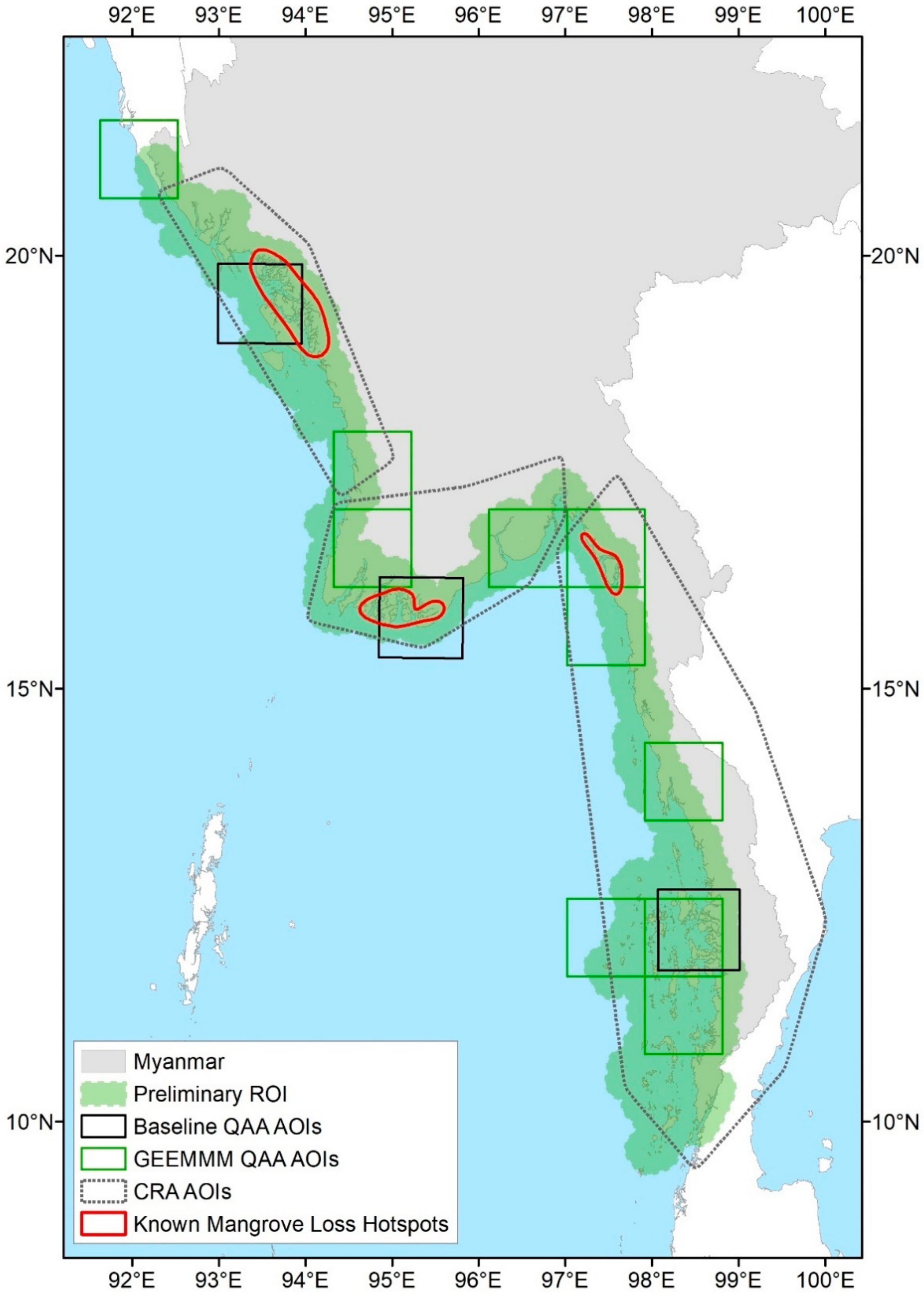
Figure 1. The preliminary region of interest (ROI) for the GEEMMM pilot representing coastal Myanmar; sub-national AOIs wherein qualitative accuracy assessments (QAAs) were untaken for existing maps (i.e., Baseline QAA AOIs); sub-national AOIs wherein GEEMMM QAAs were undertaken (i.e., GEEMMM QAA AOIs). Also shown are sub-national AOIs wherein classification reference areas (CRAs) were derived (i.e., CRA AOIs) and the location of known mangrove loss hotspots based on existing studies (i.e., Giri et al. [70], Saah et al. [73], GMW (Bunting et al. [74]), De Alban et al. [57], Clark Labs [75].
Remotesensing 12 03758 g001
Figure 2. The appearance of a typical mangrove-dominated area in Myanmar across all of the available mangrove-specific spectral indices (i.e., CMRI, MMRI, SMRI, MRI) in the GEEMMM [91].
Remotesensing 12 03758 g002
Figure 3. The appearance of all targeted classes in highest observable tide (HOT), lowest observable tide (LOT), key spectral indices, and fine spatial resolution satellite imagery viewable in Google Earth Pro (Google, Mountain View, CA, USA) [79]. The HOT and LOT composites represent 432 (R: NIR, G: red, B: green) or 453 (R: NIR, G: SWIR, B: red) false color. The spectral indices include enhanced vegetation index (EVI—[101]), combined mangrove recognition index (CMRI—[98]) and modified normalized difference water index (MNDWI—[87]).
Remotesensing 12 03758 g003
Figure 4. Comparison of distribution for all existing single- and multi-date mangrove distribution maps for Myanmar, including results of GEEEMMM pilot.
Remotesensing 12 03758 g004
Figure 5. Examples of image composite outputs from the GEEMMM showing lowest observable tide (LOT), panel (a) and highest observable tide (HOT), panel (b). The north oriented, false colour (R: NIR G: SWIR B: Red) Landsat image is over Kaingthaung Island, Ayeyarwady Region, Myanmar.
Remotesensing 12 03758 g005
Figure 6. National overview of image composite outputs from the GEEMMM showing highest observable tide (HOT) and lowest observable tide (LOT) (false color composites, R: NIR, G: SWIR, B: Red). The composites were further reduced in area using topographic and combined water masks. (A) Contemporary HOT; (B) Contemporary LOT; (C) Historic HOT; (D) Historic LOT.
Remotesensing 12 03758 g006
Figure 7. The spectral separability of all target classes as represented by CRAs across Landsat red (B1), green (B2), blue (B3), NIR (B4), SWIR1 (B5), and SWIR2 (B7) bands. The set of bar and whisker plots shows the min, max, and interquartile range.
Remotesensing 12 03758 g007
Figure 8. Example of index-specific overview of spectral values by land-cover class as represented by CRAs. MMRI is shown for each the historic and contemporary HOT and LOT datasets. The bar-whisker plots represent the min, max, and interquartile range (IQR) for each class.
Remotesensing 12 03758 g008
Figure 9. (Left) panels: Known mangrove loss hotspots (Figure 1). (Top left) shows loss, persistence, and gain (LPG) from 2004–2008 to 2014–2018 in Rakhine State; (middle left) panel shows the Ayeyarwady Region; (bottom left) shows Tanintharyi Region. (Right) Panel: contemporary high tide (HOT) image composite, false colour (R: NIR G: SWIR B: Red) with boundaries of left panels highlighted in cyan.
Remotesensing 12 03758 g009
Table 1. Inventory and summary of existing national-level mangrove datasets for Myanmar—July 2020.
Author(s)Year(s)Spatial Extent/ResolutionAvailabilityImagery Source(s)MethodsDiscrete/Continuous
Giri et al. [70]1975, 1990, 2000, 20056 tsunami-affected countries/30 mAvailable from authorsLandsatHybrid supervised/unsupervised classification (ISODATA† clustering)Discrete
SERVIR-Mekong Regional Land-Cover Monitoring System—Saah et al. [73]1987–2018 (V3)Greater Mekong region/30 mDownloadable from SERVIR-Mekong website (at c. 120 m resolution; available from authors at 30 m)Landsat, MODISSupervised classification (Support Vector Machine; Random Forest)Discrete
Global Mangrove Watch—Bunting et al. [74]1996, 2007–2010, 2015–2016Global/25 mDownloadable from Ocean Data ViewerJers-1, ALOS, ALOS-2, LandsatSupervised classification (Random Forest); histogram thresholding [57]Discrete
de Alban et al. [57]1996, 2007, 2016National/30 mAvailable from authorsLandsat, JERS-1, ALOS, ALOS-2Supervised classification (Random Forest)Discrete
Stibig et al. [76]1998–2000S and SE Asia/1 kmDownloadable from JRCSPOT-4Unsupervised maximum likelihood classificationDiscrete
Blasco et al. [77]1999Bangladesh and Myanmar/20 mNot availableSPOT 1, 2, 3Visual interpretation and supervised classificationDiscrete
Clark Labs [75]1999, 2014, 2018Multi-national/30 mDownloadable from Clark Labs websiteLandsatMahalanobis classifier; hybrid supervised/ISOCLUST clusteringDiscrete
World Atlas of Mangroves (WAM)—Spalding et al. * [5]2000–2007Global/30 mDownloadable from Ocean Data ViewerLandsatNot disclosedDiscrete
Mangrove Forests of the World (MFW)—Giri et al. [44]2000Global/30 mDownloadable from Ocean Data ViewerLandsatHybrid supervised/unsupervised classification (ISODATA clustering)Discrete
CGMFC-21—Hamilton and Casey [78]2000–2014Global/30 m2000–2012 data downloaded from CGMFC-21, 2013–2014 data available from authorsLandsatMasked Global Forest Change (GFC) [47] maps using MFW [47]) to calculate dynamicsContinuous
Richards and Friess [47]2000, 2012SE Asia/30 mNot availableLandsatMasked GFC maps using MFW [56] to calculate lossContinuous
Estoque et al. [56]2000, 2014National/30 mNot availableLandsatUnsupervised classification (ISODATA clustering)Discrete
* WAM data over Myanmar from Ministry of Forestry’s Remote Sensing and GIS Section, derived from Landsat imagery 2000–2007. Iterative Self-Organizing Data Analysis Techniques. Iterative Self-Organizing Clustering.
Table 2. Summary of GEEMMM user inputs and selected variables used in the Myanmar pilot.
GEEMM User Inputs.
ModuleInputTypeSelected Variables
Module 1Preliminary ROIDataset (vector)GUI Generated
Known Mangrove ExtentDataset (raster)Giri et al. [44]
Coast LineDataset (vector)GADM—Myanmar [82]
Digital Surface ModelDataset (raster)JAXA-ALOS DSM (30 m) [81]
Contemporary Year(s)Date range (YYYY)2014–2018
Historic Year(s)Date range (YYYY)2004–2008
Month(s)Date range (MM)06–12
Cloud Cover LimitInteger (%)30%
Cloud Cover MaskVariableAggressive
Tidal ZoneNumeric (m)1500 m
Water MaskVariableCombined
Fringe MangrovesBooleanFalse (not included)
Topographic MaskVariableUses Known Mangrove Extent [44]
Module 2Classification Reference Areas (CRAs)Dataset (vector)See Table 4
Class NamesVariableSee Table 4
Class NumbersIntegerDefined by Authors
Classification Algorithm Random ForestRandom Forest [82]
Number of TreesInteger200
Output Classification MapsVariableHist. and Cont. Combined
Module 3Classification Reference Areas (CRAs)Dataset (vector)See Table 4
Class NamesVariableSee Table 4
Class NumbersIntegerDefined by Authors
Classification ViewVariableSee Figure 7
Mangrove Class Number(s)IntegerDefined by Authors
Table 3. List of all spectral indices available in the GEEMMM including mangrove-specific.
IndexAbbreviationCalculationCitation
Simple RatioSRNIR/RedJordan [95]
Normalized Difference Vegetation IndexNDVI(NIR − Red)/(NIR + Red)Tarpley et al. [96]
Normalized Difference Water IndexNDWI(Green − NIR)/(Green + NIR)Gao [97]
Modified Normalized Difference Water IndexMNDWI(Green − SWIR1)/(Green + SWIR1)Xu [87]
Combined Mangrove Recognition IndexCMRI *NDVI − NDWIGupta et al. [98]
Modular Mangrove Recognition IndexMMRI *(|MNDWI| − |NDVI|)/(|MNDWI| + |NDVI|)Diniz et al. [43]
Soil-Adjusted Vegetation IndexSAVI1.5*(NIR − Red)/(NIR + Red + 0.5)Huete [99]
Optimized Soil-Adjusted Vegetation IndexOSAVI(NIR − Red)/(NIR + Red + 0.16)Rondeaux et al. [100]
Enhanced Vegetation IndexEVI2.5*((NIR − red)/NIR + 6*Red − 7.5*Blue + 1))Huete et al. [101]
Mangrove Recognition IndexMRI *|GVI(l) − GVI(h)|*GVI(l)* (WI(l) + WI(h))Zhang and Tian [93]
Submerged Mangrove Recognition IndexSMRI *(NDVI(l) − NDVI(h))* ((NIR(l) − NIR(h))/(NIR(h))Xia et al. [29]
Land Surface Water IndexLSWI(NIR − SWIR1)/(NIR + SWIR1)Chandrasekar et al. [102]
Normalized Difference Tillage IndexNDTI(MIR − SWIR2)/(MIR + SWIR2)Van Deventer et al. [103]
Enhanced Built-up and Bareness IndexEBBI(SWIR1 − NIR)/(10*√(SWIR1 + LWIR))As-syakur et al. [104]
* denotes mangrove-specific spectral index.
Table 4. Names and description of classes and numbers of classification reference areas (CRAs). Also shown is how many CRAs were derived within each sub-national CRA AOI (Figure 1).
ClassClass DescriptionContemporaryHistoric
AOI 1AOI 2AOI 3TotalAOI 1AOI 2AOI 3Total
Non-Forest VegetationGrass and/or shrubs dominate; some exposed soil + scattered trees; canopy < 30% closed; active cropland, vegetation appears green10872537010
Terrestrial ForestForested areas; canopy > 30% closed (includes plantations (e.g., palm))10872519010
Closed-Canopy MangroveTall, mature stands; canopy > 60% closed121693791010
Open-Canopy MangroveShort-medium stands; canopy 30–60% closed63211010010
Exposed/BarrenSoil/sediment/sand dominates; includes senesced/unhealthy (i.e., inactive) crops, mudflats, recently deforested areas4441224410
Residual WaterWater areas missed from masking4331034411
120 61
Table 5. Comparison of single- and multi-date datasets based on mapped classes, accuracy, mangrove distribution (ha), dynamics, and known limitations. Accuracy: OA = overall accuracy; UA = user’s accuracy; PA = producer’s accuracy.
Dataset/Author(s)YearExtent (ha)Dynamics (ha, %)Discrete/ContinuousMapped ClassesAccuracyKnown Limitations
Giri et al. [70]1975851,452−300,091
−35.2%
Discrete4 classes including MangrovePositional root mean square error of ± 1/2 pixelSemantic differences in class definitions, positional, and classification errors. Mangrove patches smaller than 1 ha not mapped likely reducing distribution figures.
2005551,361
SERVIR-Mekong (Saah et al. [73])19871,197,325−195,227
−16.3%
Discrete21 classes including MangroveOA 76% (2016 map)Gap in 2012 data due to removal of ETM+ imagery following Landsat 7 Scan Line Corrector failure. 2012 primitives interpolated using Whittaker smoothing algorithm. Bias in reference data toward more recent past, due to availability of high-resolution imagery.
20181,002,098
GMW (Bunting et al. [74])1996537,428−43,208
−8.0%
DiscreteMangrove presence vs no presenceOA 95.3% (2010 baseline map)Fine-scale features commonly misclassified, e.g., aquaculture features, riverine environments, and coastal fringes. Minimum mapping unit of 1 ha suggested for end user mapping.
2016494,220
De Alban et al. [57]19961,323,300−694,600
−52.5%
Discrete10 classes including Mangrove1996: OA 85.6%
Mangrove UA 92.3%
Mangrove PA 93.1%
2016: OA 89.2%
Mangrove UA 97.5%
Mangrove PA 75.0%
No significant limitations disclosed.
2016628,700
Clark Labs [75]1999703,945−76,465
−10.9%
Discrete7 classes including MangroveOA 96.9%
Mangrove UA 98.11%
Mangrove PA 93.04%
No significant limitations disclosed.
2018627,48033 classes including Mangrove2014: OA 93.7%
Mangrove UA 94%
Mangrove PA 92%
Blasco et al. [77] 1999690,000n/aDiscrete8, including 6 mangrove classesNot disclosedLimitations with use of ‘quick look’ data due to modest technical performance. The authors state that classification accuracy could be improved by 10% if NDVI and empirical thresholds were included.
MFW (Giri et al. [44])2000494,584n/aDiscreteMangrove presence vs no presencePositional root mean square error of ±1/2 pixelSmall patches of mangrove (<0.09–0.27 ha) not well captured.
CGMFC-21 (Hamilton and Casey [78])2000279,260−27,064
−9.7%
ContinuousMangrove canopy coverPositional root mean square error of ±1/2 pixelPixels containing just 0.01% forest canopy cover are included as mangrove falling well below commonly used minimum canopy cover definitions (e.g., [78,118,119]).
2014252,196
Richards and Friess [47]2000502,466−27,770
−5.5%
ContinuousMangrove deforestationPositional root mean square error of ±1/2 pixelReported figures reflect rates of mangrove loss rather than net mangrove change, likely reducing areal figures.
2012474,696
Estoque et al. [56]2000666,759−191,122
−28.7%
DiscreteMangrove presence vs no presence2000: OA 91%
2014: OA 97%
No significant limitations disclosed.
2014475,637
WAM (Spalding et al. [5] *)2004502,911n/aDiscreteNot disclosedNot disclosedNo significant limitations disclosed.
GEEMMM (Yancho et al., 2020)2004–2008995,411−352,752
−35.4%
Discrete6 classes including combined Mangrove.2004–2008: OA 97.01%
2014–2018: OA 96.08%
Refer to Results and Discussion; Conclusion.
2014–2018642,659
* WAM data over Myanmar from Ministry of Forestry’s Remote Sensing and GIS Section, derived from Landsat imagery 2000–2007.
Table 6. Results of QAA for available/acquired datasets (1 = best).
RankDatasetAOI 1—RakhineAOI 2—AyeyarwadyAOI 3—TanintharyiOverall RepresentationComments
1Clark Labs [75]Well-representedWell-representedWell-representedWell-representedMangrove very well-represented
2De Alban et al. [57]Under-representedUnder-representedWell-representedUnder-representedMangrove slightly under-represented; some confusion between cropland and mangrove
3MFW
(Giri et al. [44])
Well-representedUnder-representedUnder-representedUnder-representedMangrove under-represented
4GMW (Bunting et al. [74])Under-representedUnder-representedWell-representedUnder-representedMangrove under-represented
5Giri et al. [70]Under-representedUnder-representedUnder-representedUnder-representedMangrove under-represented, considerably in places
6SERVIR-Mekong (Saah et al. [73])Under-representedUnder-representedUnder-representedUnder-representedMangrove under-represented, considerably in places
Table 7. Final Historic and Contemporary Validation Error Matrices, using validation CRAs pixels.
Historic Classification Validation Error Matrix
Terrestrial ForestMangroveExposed/BarrenResidual WaterNon-Forest VegetationTotalUser’s Accuracy
Terrestrial Forest24000024100.0
Mangrove05400054100.0
Exposed/Barren00250025100.0
Residual Water00033033100.0
Non-Forest Vegetation0410263183.9
Total2458263326167
Producer’s Accuracy100.093.196.2100.0100.0
Overall Accuracy 162/16797.0
Contemporary Classification Validation Error Matrix
Terrestrial ForestMangroveExposed/BarrenResidual WaterNon-Forest VegetationTotalUser’s Accuracy
Terrestrial Forest7700027997.5
Mangrove112200012399.2
Exposed/Barren00330033100.0
Residual Water00024024100.0
Non-Forest Vegetation2000717397.3
Total80122332473327
Producer’s Accuracy96.3100.0100.0100.097.3
Overall Accuracy 327/33298.5
Publisher’s Note: MDPI stays neutral with regard to jurisdictional claims in published maps and institutional affiliations.