The Ultra-Short-Term Forecasting of Global Horizonal Irradiance Based on Total Sky Images

Abstract

Solar photovoltaics (PV) has advanced at an unprecedented rate and the global cumulative installed PV capacity is growing exponentially. However, the ability to forecast PV power remains a key technical challenge due to the variability and uncertainty of solar irradiance resulting from the changes of clouds. Ground-based remote sensing with high temporal and spatial resolution may have potential for solar irradiation forecasting, especially under cloudy conditions. To this end, we established two ultra-short-term forecasting models of global horizonal irradiance (GHI) using Ternary Linear Regression (TLR) and Back Propagation Neural Network (BPN), respectively, based on the observation of a ground-based sky imager (TSI-880, Total Sky Imager) and a radiometer at a PV plant in Dunhuang, China. Sky images taken every 1 min (minute) were processed to determine the distribution of clouds with different optical depths (thick, thin) for generating a two-dimensional cloud map. To obtain the forecasted cloud map, the Particle Image Velocity (PIV) method was applied to the two consecutive images and the cloud map was advected to the future. Further, different types of cloud fraction combined with clear sky index derived from the GHI of clear sky conditions were used as the inputs of the two forecasting models. Limited validation on 4 partly cloudy days showed that the average relative root mean square error (rRMSE) of the 4 days ranged from 5% to 36% based on the TLR model and ranged from 12% to 32% based on the BPN model. The forecasting performance of the BPN model was better than the TLR model and the forecasting errors increased with the increase in lead time.

1. Introduction

Solar photovoltaics (PV) is developing at an unprecedented speed, which is attributed to dramatic cost reductions, technology advancements and government policy support [1,2,3]. According to the IEA (International Renewable Energy Agency) report, global solar PV power generation increased by 22% to 720 TWh in 2019 [4]. However, the ability to forecast PV power remains a key technical challenge for the integration of large-scale PV into the electrical grid due to the variability and uncertainty of solar irradiance, which affects PV power most directly [5,6,7,8,9]. Moreover, accurate forecasting of solar irradiance is crucial to the dispatch and management of power systems [5]. Further ultra-short-term systems for forecasting highly spatially and temporally resolved solar irradiance in a timeframe of 15 min have been put forward to optimize the operation of solar power plants [10,11,12]. In fact, the amount of GHI (global horizontal irradiance) is closely related to atmospheric conditions including cloud, transparency, aerosol concentration and water content [13], in which cloud is the most dominant factor [14,15], and rapid fluctuations of GHI are generally caused by large changes in cloud conditions [16]. At present, the forecasting of cloud fraction and location is very difficult according to physical and dynamics principles, although it is vital to the ultra-short-term forecasting of solar irradiance [17].

Although well-established methods have been developed for operational solar irradiance forecasting, in the previous studies, part of solar irradiance forecasting applications based on statistical models or artificial neural networks do not directly use characteristic information of cloud, resulting in significant biases [18,19,20,21,22], and the numerical weather prediction (NWP) models that can infer local cloud cover information through the dynamic modeling of atmosphere are widely used for solar irradiance forecasting of several hours to a few days ahead [23,24], whereas they are unlikely to capture real-time temporal relationships between solar irradiance and meteorological factors and simulate cloud with severe convection or short life cycle, due to the coarse spatial resolutions and uncertain initial conditions of NWP models and complicated microscopic physical characteristics of cloud particles [10,25], eventually leading to random errors in short-term solar irradiance prediction [26,27,28]. Satellite-based solar irradiation forecasting of 1–6 h ahead does not have adequate fine temporal and spatial resolutions to extract information of small-scale and low-altitude cloud [29]. Hence, ground based remote sensing with high temporal and spatial resolution was developed for solar irradiation forecasting to fill the gap of NWP and satellite-based models in nowcasting applications [30,31].

In recent years, sky imagers that rely on ground measurements combined with irradiance sensors have been widely used for nowcasting systems. For Total Sky Imager (TSI), cloud indices derived from images were used for nowcasting of GHI and were reported to have potential for solar irradiance forecasting of 15–20 min ahead [30]. Furthermore, the intra hour forecasting applications for direct normal irradiance (DNI) or GHI of 20 min ahead were performed and the results showed better performance than the persistence model; these studies generally combined the TSI images and the cloud base height for cloud tracking [32,33,34]. Other studies, in which predictive cloud indices inferred from the ground-based measurements were applied to artificial neural network (ANN) or multilayer-perceptron-network (MLP) models, improved intra hour irradiance forecasting results [35,36]. The radiative transfer model was combined with predicted sky images to forecast GHI and DNI for time horizons of 1–10 min ahead [37]. Recently, minutely solar irradiance was forecasted though the mapping relationship between sky images and irradiance [38]. Moreover, raindrop detection for sky images was proposed to improve the accuracy of short-term solar irradiance [39]. It is obvious that various technologies can be applied to sky images for short-term solar irradiance.

The goal of this paper is to establish two ultra-short-term rolling forecasting models of GHI based on Ternary Linear Regression (TLR) and Back Propagation Neural Network (BPN) using the observation of a sky imager (TSI-880) and GHI in Dunhuang, China. The TLR model was used to establish the real-time temporal linear relationship between three different sky types (thick cloud, thin cloud and clear sky) derived from images and the clear sky index derived from clear sky model, to determine the attenuation proportion of the three sky types to the clear sky index, while the BPN model was used for constructing the nonlinear relation between cloud and clear sky index to forecast GHI.

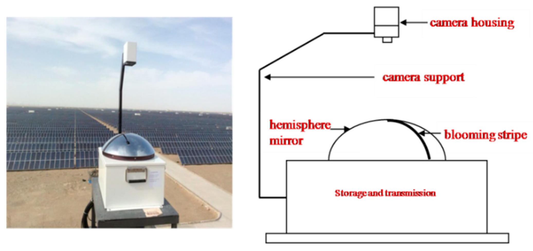
2. Instruments and Data

The Total Sky Imager of TSI-880 deployed on the rooftop of a solar plant in Dunhuang (set up at 94.478°E, 40.078°N, 1221 m MSL (mean sea level)) was mainly used for ultra-short-term forecasting of the power generation of photovoltaics. The appearance and composition of TSI-880 are shown in Figure 1, consisting of a sun tracking and blocking device, imaging device, and a built-in micro-computer used for the storage and transfer of data. The dome of mirror rotates at a certain speed to ensure that the shadow band blocks strong direct sunlight and prevents the lens from being damaged, and captures the sky scene reflected on the hemisphere mirror with a downward charge coupled device (CCD) camera.

A solar shortwave radiation meter of TBQ-2 was used to measure the instantaneous GHI accurately. The images with a resolution of 352 × 288 pixels and a 24-bit color JPEG format and GHI data were sampled synchronously with the frequency of 1 min, and simultaneously stored locally and remotely to guarantee the timeliness, integrity and reliability of the data.

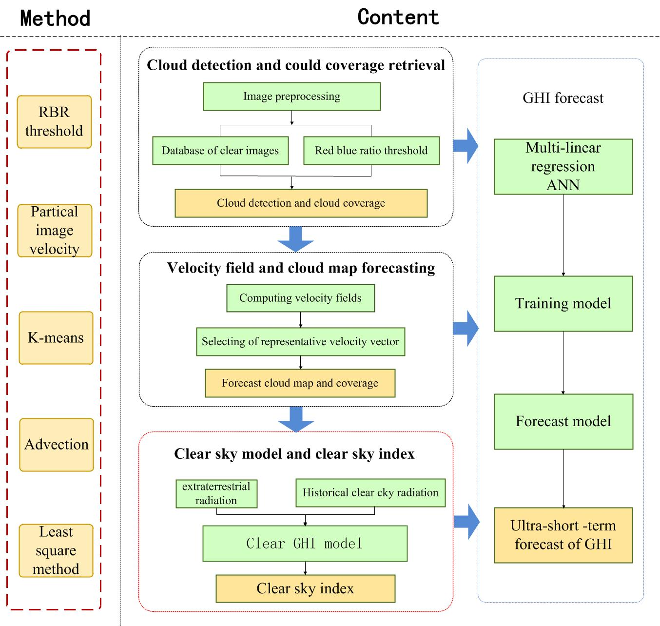
3. Methods and Results

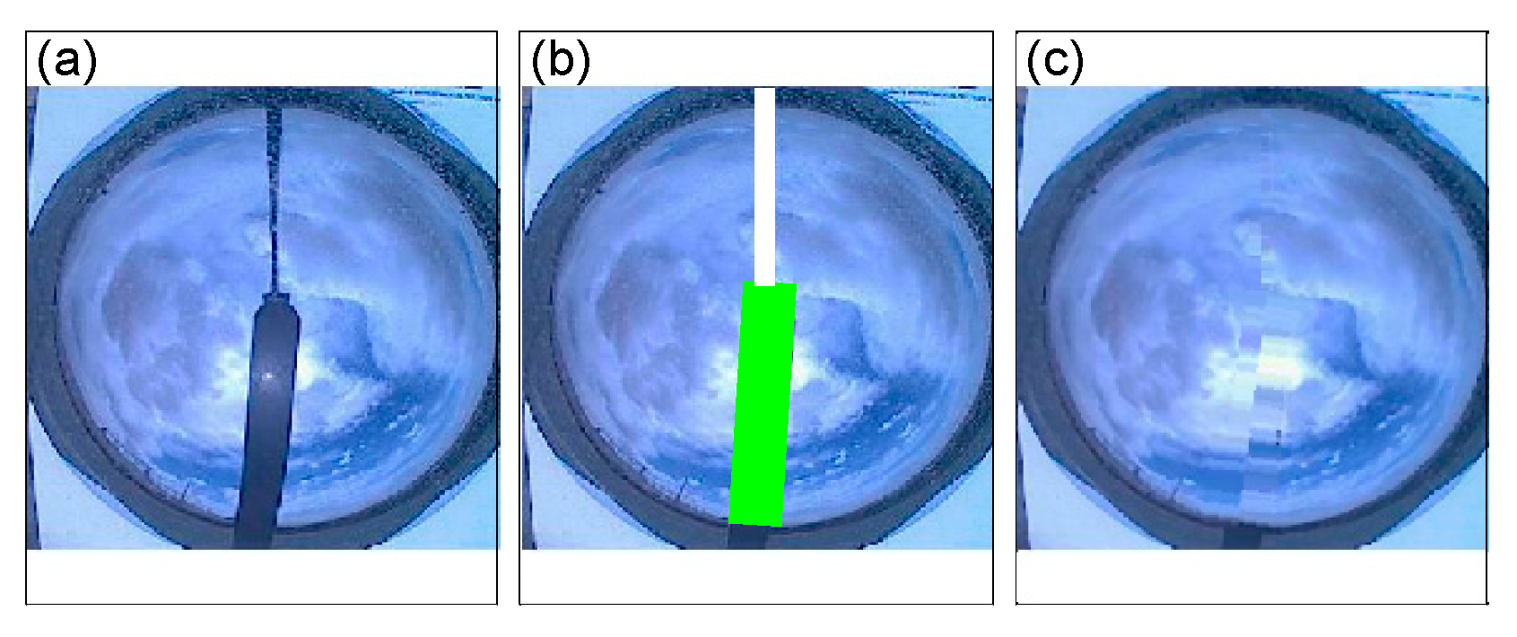
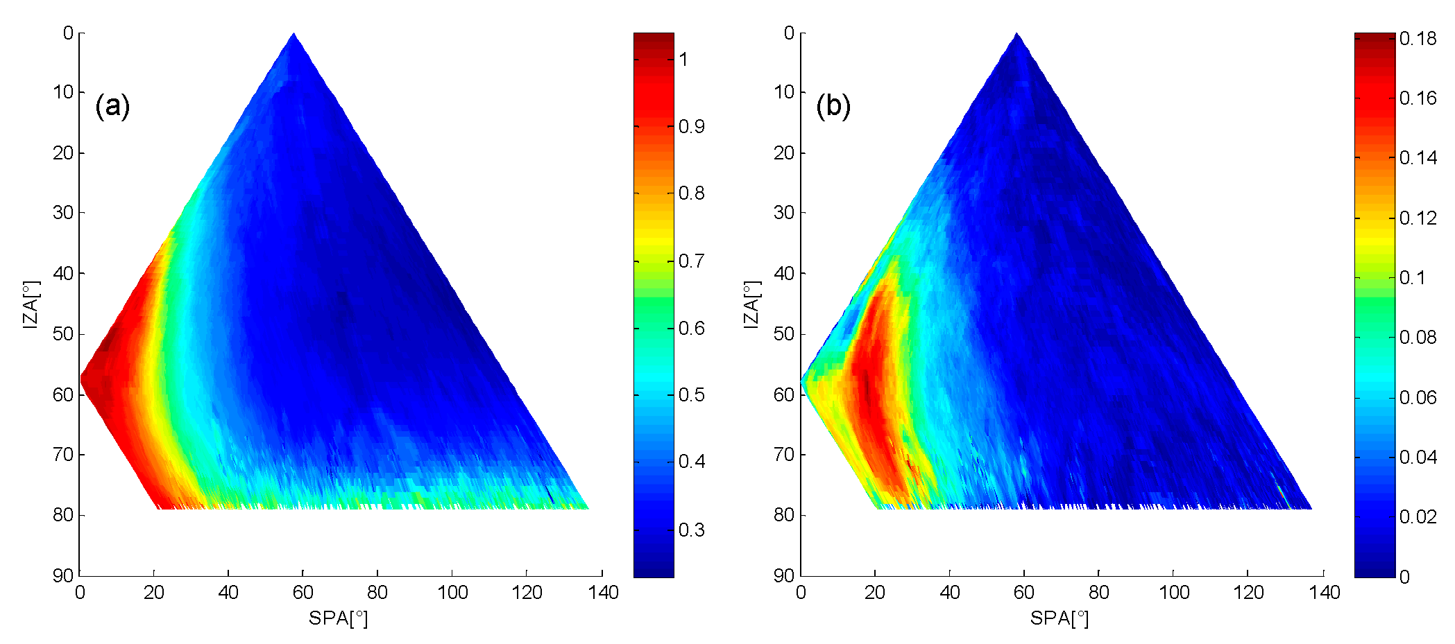
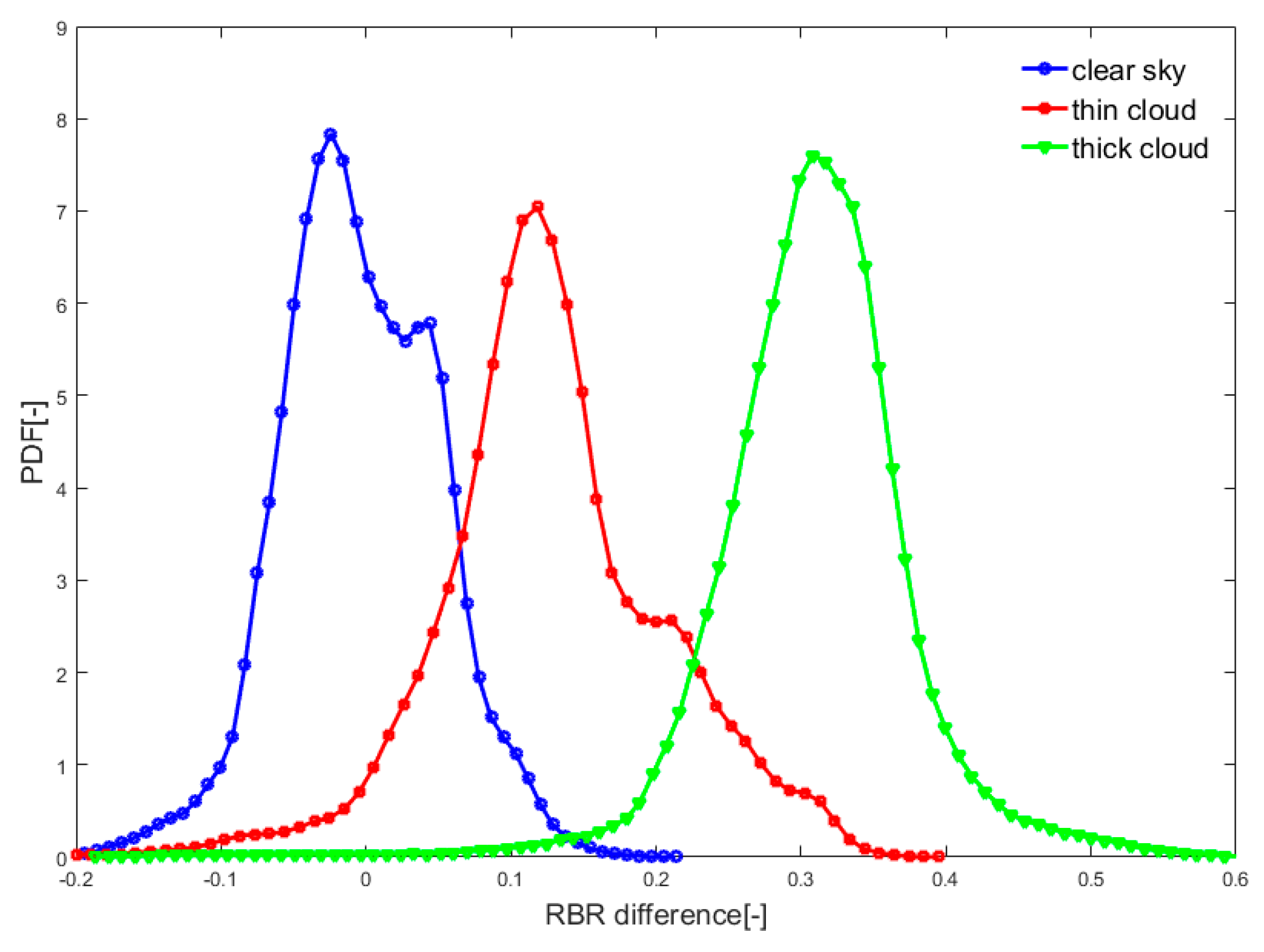
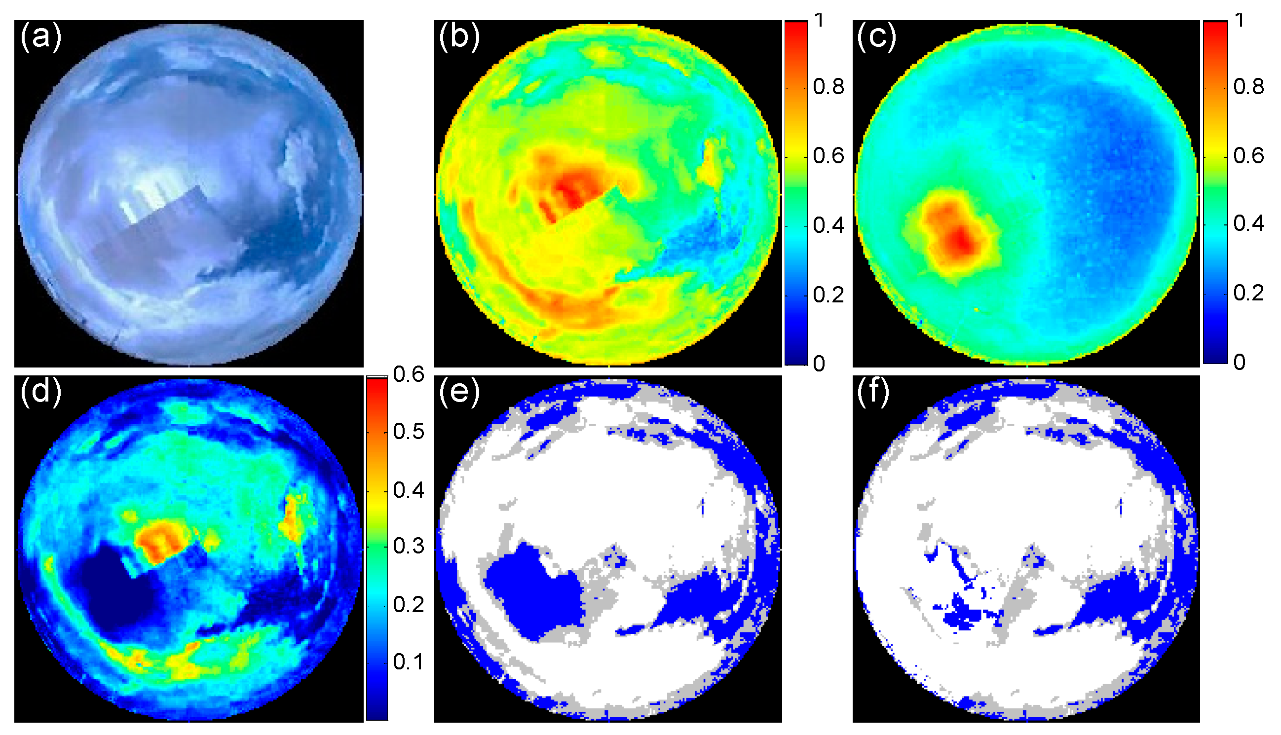
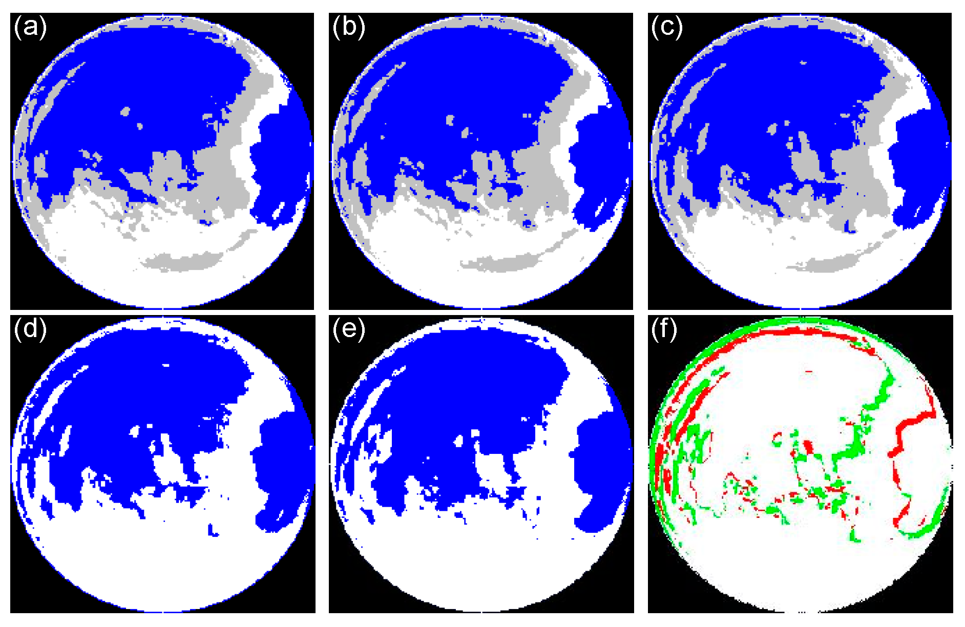
3.1. Cloud Detection and Retrieve

Feature extraction from cloud images is a key component in the application of the Total Sky Imager [12]. Although TSI-880 provides cloud detection according to the built-in algorithm, the single fixed red-blue-Ratio (RBR) threshold for all images and untreated shielding caused significant error in the results. To be specific, on the one hand, the cloud information near the sun shielded by the shadow band is vital for ultra-short-term irradiance forecasting [34]. On the other hand, the image RBR is greatly affected by atmospheric conditions including transparency, aerosol content and sand dust, even though for the same clear sky image, the RBR values around the sun and near the horizon are larger due to aerosol forward scatter and long optical path [40,41]. Given this, we performed cloud detection based on the RBR threshold to determine the cloud fraction.

The first step of cloud detection is recovering the shielding areas that result from the support arm and shadow band, as shown in Figure 2a. The angle of the shadow band deviates from the true north on the image, which is equal to the solar azimuth (SAA), because projection of the sky on the image is isometric [42], and the area of shadow band is shown in the green area of Figure 2b and interpolated according to the pixels on both sides. The projection of the support arm with a fixed position is shown in the white area of Figure 2b and is restored by horizontal bidirectional interpolation. The restored image is shown in Figure 2c. Additionally, the sky, effectively occupying 260 × 260 pixels, is cropped from the original image and distortion is corrected by the spherical distortion correction model [43].

In the TSI spherical coordinate system, the relationship of the zenith angle, azimuth and scattering angle (marked with $\Theta$) is shown in Figure 3. The small black square indicates a point on the spherical mirror, ${\theta }^{\prime }$ and ${\varphi }^{\prime }$ are the zenith angle (IZA) and the azimuth angle of the point, respectively; $\theta$ and $\varphi$ are the solar zenith angle (SZA) and SAA, respectively. The IZA is used to represent the zenith angle of the pixel on the image, and the SPA (Sun-Pixel Angle) is the angle between the sun and the pixel, representing the positional relationship between the pixel and the sun on the image. The SPA is approximately equal to $\Theta$ due to the long distance between the sun and the earth. From Figure 3, we have:

$$\sin (IZA)=\sin {\theta }^{\prime }=\frac{r}{R}$$

(1)

$$\cos (SPA)=\cos \Theta =\cos \theta \cos {\theta }^{\prime }+\sin \theta \sin {\theta }^{\prime }\cos \left(\varphi -{\varphi }^{\prime }\right)$$

(2)

where r is the distance between pixel and image center on the image, and R is the radius of the image.

The images with the SZA of 58° under clear-sky conditions were selected for representing the relationship of the RBR, IZA and SPA, as shown in Figure 4a. It is obvious that the RBR values decrease with the increase in SPA, while they increase with the increase in IZA. The areas of near horizon (IZA > 75°) and around the sun (SPA < 35°) have larger values of RBR in relation to other areas. Hence, the Clear Sky Library (CSL) was applied to eliminate the dependence of RBR on the areas around the sun and horizon [45]. To be specific, the historical clear images were selected as background images to provide RBR reference for images to be detected, and SZA, IZA, SPA, R, G, and B brightness values of historical clear images were saved as the data fields of the CSL. Additionally, we calculated the standard deviation distribution of the RBR of different clear sky images (Figure 4b) and found that the RBR variation had a large range from 0.1 to 0.18 in the area around the sun (SPA < 35°). Given this, the closest image in the CSL was selected for the images to be detected, to reduce the impact of aerosols concentration and sun position projection on the RBR.

As for the thresholds of different sky types, a certain number of images taken on different dates during the observation were selected as training samples. The thresholds shown in Figure 5 were derived from the PDF (probability distribution function) of RBR differences of pixels between the selected images of CSL and the sample images, and the thresholds of clear sky (T_clear) and thick cloud (T_thick) were 0.067 and 0.225, respectively.

A pixel was identified as thick cloud if the difference of RBR between the pixel and the corresponding pixel in the background image ($\Delta \mathrm{RBR}$) was larger than 0.225; if the $\Delta \mathrm{RBR}$ was smaller than 0.067, the pixel was identified as clear sky, otherwise the pixel was identified as thin cloud. An instance of cloud detection is shown in Figure 6e. Moreover, the sun parameter (SP) proposed by Pfiste et al. [16] was introduced to correct the type of the pixels around the sun. SP is a dynamic single threshold defined as the RBR average of the pixels around the sun (Figure 4a, −35° < SPA <35°). If the sun is obscured by thick cloud (Figure 6a), RBR of the pixels around the sun are usually smaller than that of the clear day, leading to misidentification as clear sky (Figure 6e). Consequently, when the RBR of the pixel around the sun was larger than the SP, the pixel was re-recognized as thick cloud (Figure 6f). Finally, the cloud fraction of thick cloud ($f_{\mathrm{thick}}$) and thin cloud ($f_{\mathrm{thin}}$) are the ratios of the numbers of thick cloud and thin cloud to total pixels, respectively.

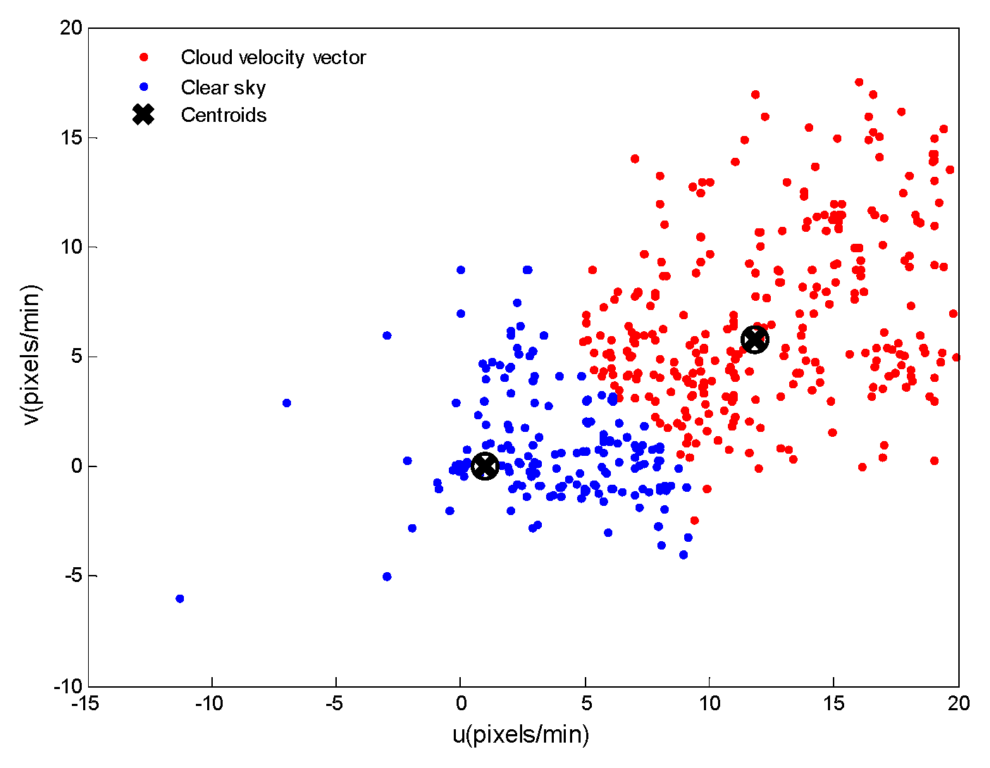
3.2. Cloud Velocity and Cloud Map Forecasting

Forecasting of the cloud map is a prerequisite for estimating solar irradiance with total sky images. The MATLAB-based algorithm “mpiv (particle image velocimetry)” developed by Mori and Chang was applied to the two consecutive images for estimating the translational speed of the cloud [46]. The algorithm has been successfully applied to cloud velocity estimation in solar irradiance forecasting with all-sky images, infrared images and satellite images [32,47,48]. To avoid errors caused by cloud detection, the red channel of the raw images was extracted to calculate cloud speed because “mpiv” can only be used for two-dimensional images, and the red channel of the image has higher contrast to clear sky and cloud than the blue and green channels. The interval of the two consecutive images was 1 min, and the search sub-window was defined as an area of 32 × 32 pixels. Two iterative recursive checks were performed using the MQD (Minimum Quadric Differences) algorithm to calculate the velocity vector field. Median filtering was used to remove discrete error vectors, and finally linear interpolation was used to correct the error vectors.

The cloud velocities were assumed to have the same direction and magnitude due to the limited sight of the TSI. For the clear sky area, the calculated velocities are usually zero or close to zero. Therefore, the calculated velocity vector fields were divided into two categories with the K-means algorithm and the larger value of cluster centers was selected as the representative velocity vector of the cloud. The red and blue scatters represent the velocity fields of the cloud and clear sky, respectively, and the black cross indicates the cluster center in Figure 7. The velocity vector of the cloud was u = 10.3, v = 7.9 (pixels/min); u and v represent the velocity of the horizontal and vertical direction, respectively.

To obtain the forecasted cloud map, the retrieved cloud map was advected to the future with the representative velocity vector. However, the information at the boundary of images is likely to be unpredictable due to the limited observation view of TSI. Here, the boundary of the forecasted cloud map was filled with the boundary information of the image 1 min ago. From Figure 8, we found that the pixels at the edge were more error-forecasted because these areas use the boundary information of the previous moment, and the pixels of thin clouds are also more error-forecasted because the thin clouds are difficult to be accurately detected in the raw image, especially in the area around the sun. The pixels of clear sky are likely to be detected as thin clouds due to the forward scattering of aerosols and haze. Therefore, the accuracy of cloud forecasting is limited by the TSI observation view and cloud detection errors.

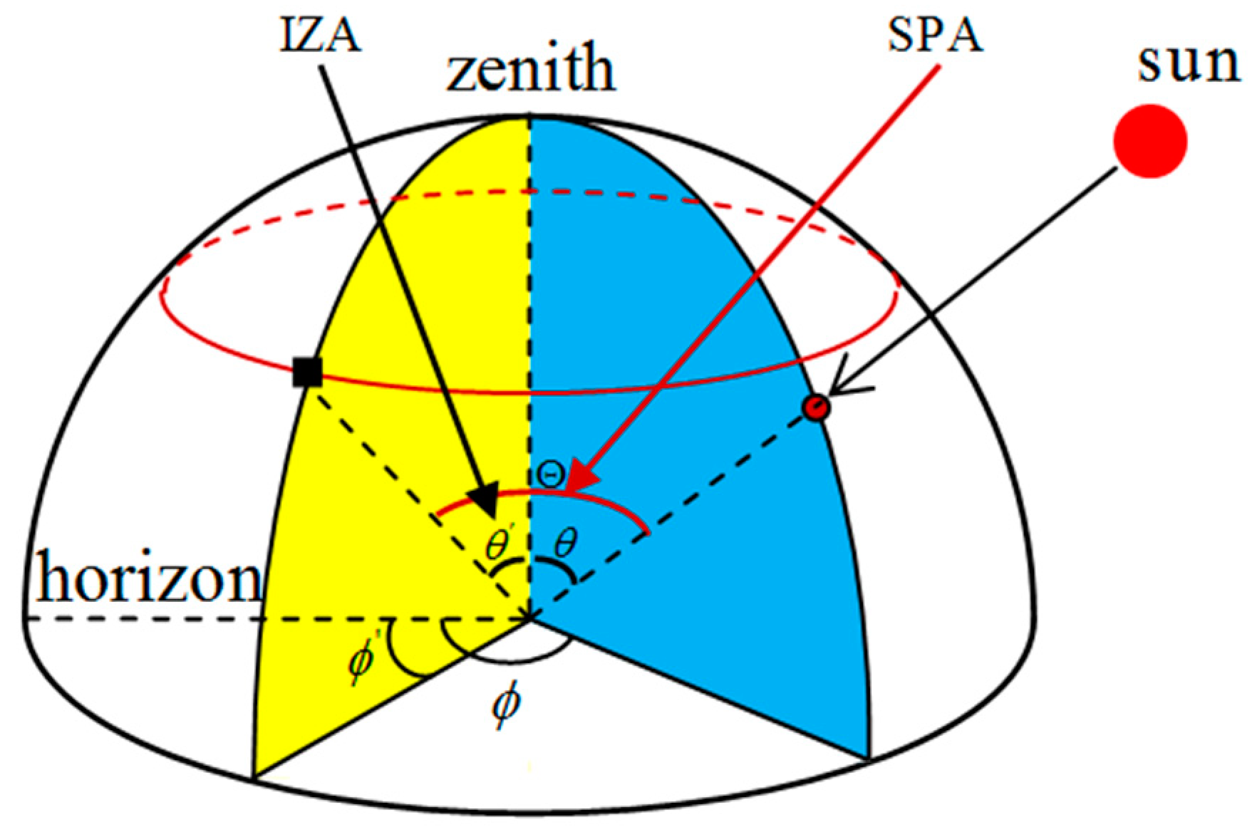
3.3. The Clear Sky Model and Clear Sky Index

Extraterrestrial solar radiation received by the upper boundary of the atmospheric layer changes with the Earth–Sun distance. For the observation site located at latitude φ and longitude λ, the extraterrestrial irradiance ($I_{\mathrm{ets}}$) at a certain moment can be calculated by the solar constant and the position of the sun at the moment:

$$I_{\mathrm{ets}}=S_c(1+0.033\times \cos (\frac{360}{365}\times d))\cos \theta$$

(3)

S_c is the solar constant (1367 W/m²) [49], d is the DOY (day of year) of the year, 1 January is 1 and 31 December is 365.

Diurnal variation of $I_{\mathrm{ets}}$ is a cosine function of the zenithal angle [50]. The GHI exhibits uniform attenuation of $I_{\mathrm{ets}}$ under conditions of clear sky, while it shows random and irregular fluctuations under conditions of broken sky with active clouds. Consequently, many irradiance forecasting models were developed from clear-sky radiation models. The existing clear-sky models such as Solis, Kasten and Ineichen typically developed from atmospheric radiative transfer models can simulate the GHI well, but usually require additional meteorological factors such as aerosol optical depth, ozone content, water vapor content and turbidity [51]. In this study, the clear-sky model was established between the $I_{\mathrm{ets}}$ and the GHI of clear days during the observation though the least square method.

$$I_{\mathrm{clk}}={\displaystyle \sum }_{n=0}^2{a}_n{\left(I_{\mathrm{ets}}\right)}^n, a_n=\left\{-0.00000476,0.8123113,-35.9099519\right\}$$

(4)

where $I_{\mathrm{clk}}$ is the GHI under clear sky, $a_n$ are fitting coefficients.

The three-dimensional radiation transmission process in the clouds and the cloud radiative effect of clouds are very complicated; it is difficult to quantify the forcing effect of clouds on radiation. The variation of GHI is assumed to be caused by changes in cloud fraction and type (thick cloud and thin cloud) due to the small observation scope. The clear sky index, defined as the ratio of GHI to $I_{\mathrm{ets}}$, is used to reflect the attenuation degree of entire atmosphere to $I_{\mathrm{ets}}$. Whereas in the studies of radiation forecasting, the clear sky index ($k_{\mathrm{t}}$) is usually defined as the ratio of GHI to clear sky GHI [31], meaning that only the effect of the cloud is considered while the influence of other radiative forcing factors, including atmospheric molecules and aerosols, is excluded. Additionally, the attenuation degree of radiation by clouds with different optical thicknesses varies considerably. Thick clouds with low-altitude can reduce DNI to almost zero in a few seconds [33], while thin clouds with high-altitude may reduce GHI by 10% [14,52]. Hence, we established GHI estimation models based on the principle of the attenuation degree of cloud to irradiance varying with the distribution proportions of the different types of sky (thick cloud, thin cloud, and clear).

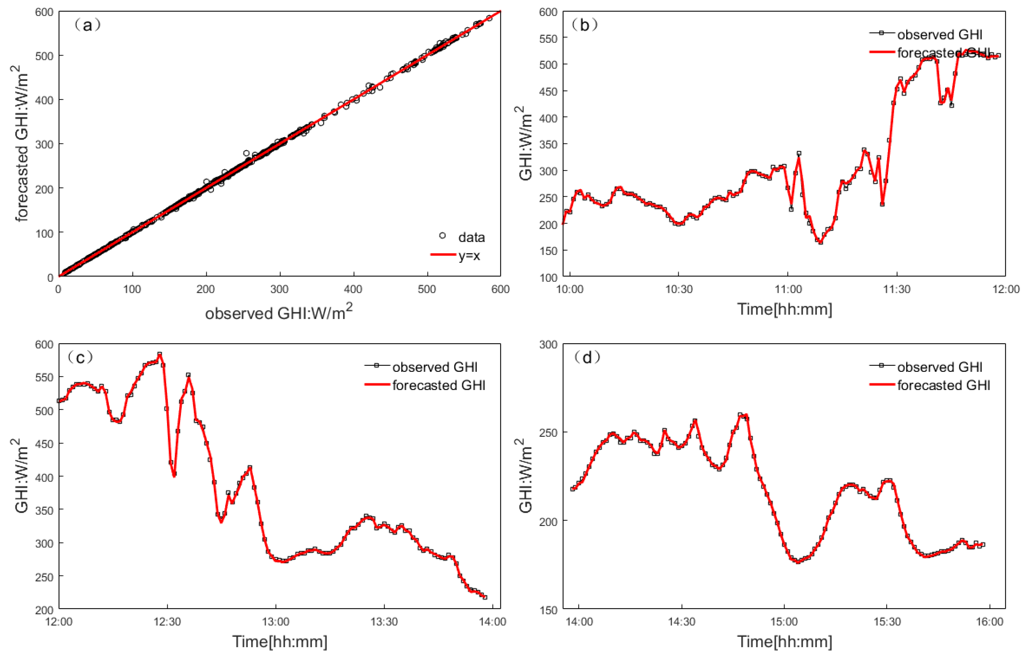
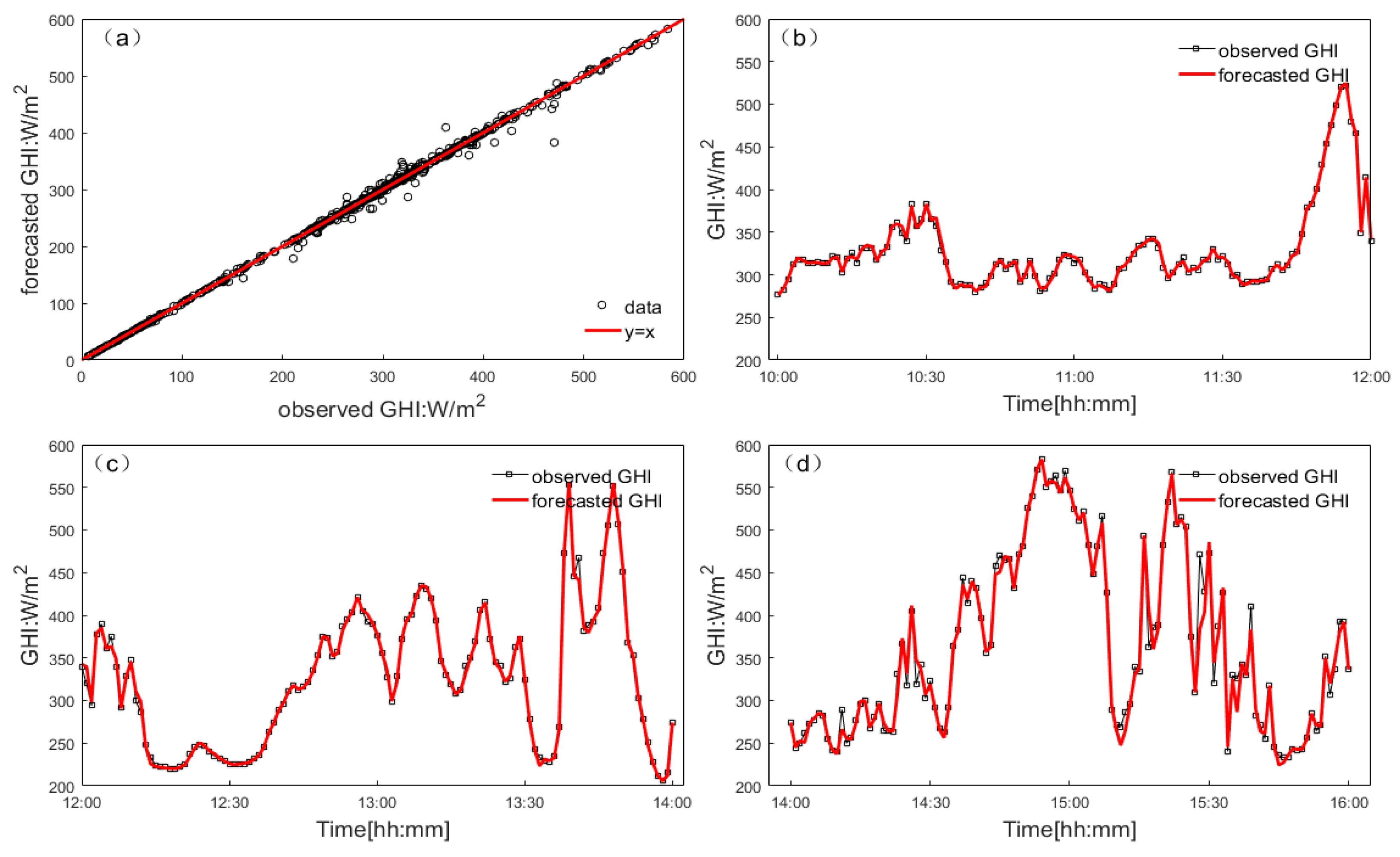
3.4. Forecasting of GHI

3.4.1. Two Forecast Models of GHI

Based on the retrieved and forecasted cloud fraction and clear sky index, the two rolling forecasting models of GHI using ternary linear regression (TLR) and BP neural network were established. Rolling forecasting refers to training the previous model with n values observed from time t-n to t, and the model is used for the forecasting of future time.

The TLR model constructed the relationships of $k_{\mathrm{t}}$ and cloud fraction as shown in Formula (5), describing the attenuation proportion of three sky types (thick cloud, thin cloud and clear sky) 5 min before forecast time, for correcting the clear sky index dynamically.

$$k_{\mathrm{t}\left(t-5\_t\right)}={\mathrm{a}}_{\left(t-5\_t\right)}+b_{1\left(t-5\_t\right)}{f}_{\mathrm{thick}\left(t-5\_t\right)}+b_{2\left(t-5\_t\right)}{f}_{\mathrm{thin}\left(t-5\_t\right)}+b_{3\left(t-5\_t\right)}{f}_{\mathrm{clear}\left(t-5\_t\right)}$$

(5)

where $f_{\mathrm{thick}}$, $f_{\mathrm{thin}}$, $f_{\mathrm{clear}}$ are the fractions of thick cloud, thin cloud and clear sky. The subscript $t-5\_t$ indicates 5 min from t − 5 to t.

The regression coefficients obtained by formula 5 combined with forecasted cloud fraction were applied to estimate the $k_{\mathrm{t}}$ and GHI of the short-term future.

$$k_{\mathrm{t}\left(t+\Delta t\right)}={\mathrm{a}}_{\left(t-5\_t\right)}+b_{1\left(t-5\_t\right)}{f}_{\mathrm{thick}\left(t+\Delta t\right)}+b_{2\left(t-5\_t\right)}{f}_{\mathrm{thin}\left(t+\Delta t\right)}+b_{3\left(t-5\_t\right)}{f}_{\mathrm{clear}\left(t+\Delta t\right)}$$

(6)

$$I_{t+\Delta t}=I_{\mathrm{clk}\left(t+\Delta t\right)}\times k_{\mathrm{t}\left(t+\Delta t\right)}$$

(7)

where, $\Delta t$ represents the forecasting time scale (taken as 0~5 min in this paper). The subscript $t+\Delta t$ represents the forecasting time.

The BP (Back Propagation) neural network is a multi-layer feed-forward neural network trained by an error back-propagation algorithm which can obtain complex non-linear processing capability through complex mapping of simple non-linear processing elements. Its basic principle is to use the gradient descent method to minimize the mean square error between the actual output and the expected output of the network. It consists of the input layer, the hidden layer, and the output layer. The hidden layer consists of several neural units and each neural unit has a randomly assigned threshold and assigns a weight to the input layer and output layer. The calculation process includes the forward propagation of the signal and the backward propagation of the error. The error output is calculated in the direction from input to output, and the weight and threshold are adjusted in the direction from output to input. In this paper, a BP neural network is used to establish a ultra-short-term GHI forecast model. The training process of the prediction model is simply expressed as Equation (10):

$$(AN{N}_u\left(L,N\right),I,T)\stackrel{\mathrm{training}}{\to }AN{N}_B$$

(8)

$AN{N}_u$ is an untrained BP neural network, $L$ is the number of hidden layers, $N$ is the number of neurons in each hidden layer. $I$ represents inputs including $f_{\mathrm{thick}\left(\mathrm{t}-10\_\mathrm{t}\right)}$, $f_{\mathrm{thin}\left(\mathrm{t}-10\_\mathrm{t}\right)}$, $I_{\mathrm{ets}}$, and $I_{\mathrm{clk}}$, and $T$ represents the target. $AN{N}_B$ is the trained BP neural network. The forecasting model is given by:

$$\widehat{I}\left(t+\Delta t\right)=AN{N}_B\left(I_n\left(t\right)\right)$$

(9)

where $I_n$ represents new inputs that do not contain the samples involved in training.

Forecasting accuracy and operating efficiency are important indicators for evaluating the performance of the ultra-short-term forecasting model due to the demand of online rolling learning. This paper selected 3, 20, and 10 for L, N and the number of samples, respectively, by training the N, L, the number of iterations and sample error and considering the accuracy of forecasting results and the efficiency of running time.

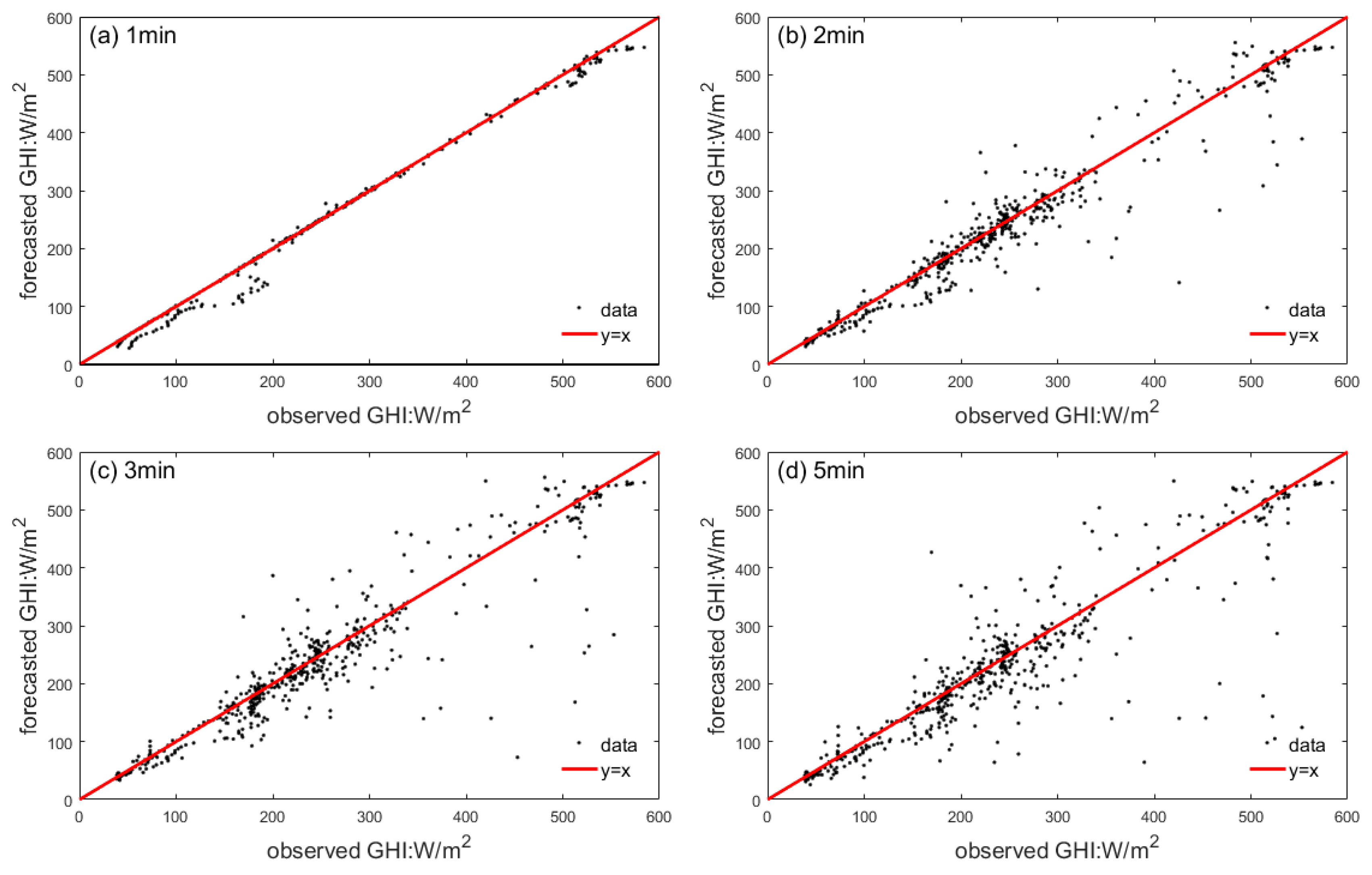
3.4.2. Evaluation of Forecast Models

Pearson correlation coefficient (R) given by formula 10 is used to evaluate the correlation between the forecasted and measured GHI:

$$R=\frac{{\sum }_{n=1}^N\left(I_{\mathrm{fh}}-\overline{I_{\mathrm{fh}}}\right)\left(I_{\mathrm{obs}}-\overline{I_{\mathrm{obs}}}\right)}{\sqrt{{\sum }_{n=1}^N{\left(I_{\mathrm{fh}}-\overline{I_{\mathrm{fh}}}\right)}^2}\sqrt{{\sum }_{n=1}^N{\left(I_{\mathrm{obs}}-\overline{I_{\mathrm{obs}}}\right)}^2}}$$

(10)

RMSE (Root Mean Square Error) and rRMSE (relative RMSE) are used to indicate the deviation degree of the predicted and measured irradiance, and smaller values for RMSE and rRMSE indicate higher forecasting accuracy and smaller deviation between the forecasted and observed GHI.

$$RMSE=\sqrt{\frac{1}{N}{\displaystyle \sum }_{n=1}^N{\left(I_{\mathrm{fh}}-I_{\mathrm{obs}}\right)}^2}$$

(11)

$$rRMSE=\sqrt{\frac{1}{N}{\displaystyle \sum }_{n=1}^N{\left(I_{\mathrm{fh}}-I_{\mathrm{obs}}\right)}^2}\times \frac{100}{\overline{I_{\mathrm{obs}}}}$$

(12)

MAE (Mean Absolute Error) is the average of absolute error of the predicted and measured GHI, which can better reflect the prediction error. MAE and rMAE (relative Mean Absolute Error) can be defined by:

$$MAE=\frac{1}{N}{\displaystyle \sum }_{n=1}^N\left(\left|I_{\mathrm{fh}}-I_{\mathrm{obs}}\right|\right)$$

(13)

$$rMAE=\frac{1}{N}{\displaystyle \sum }_{n=1}^N\left(\left|I_{\mathrm{fh}}-I_{\mathrm{obs}}\right|\right)\times \frac{100}{\overline{I_{\mathrm{obs}}}}$$

(14)

MBE (Mean Bias Error) is the average value of the predicted and measured GHI errors; MBE and rMBE (relative Mean Bias Error) are given by:

$$MBE=\frac{1}{N}{\displaystyle \sum }_{n=1}^N\left(I_{\mathrm{fh}}-I_{\mathrm{obs}}\right)$$

(15)

$$rMBE=\frac{1}{N}{\displaystyle \sum }_{n=1}^N\left(I_{\mathrm{fh}}-I_{\mathrm{obs}}\right)\times \frac{100}{\overline{I_{\mathrm{obs}}}}$$

(16)

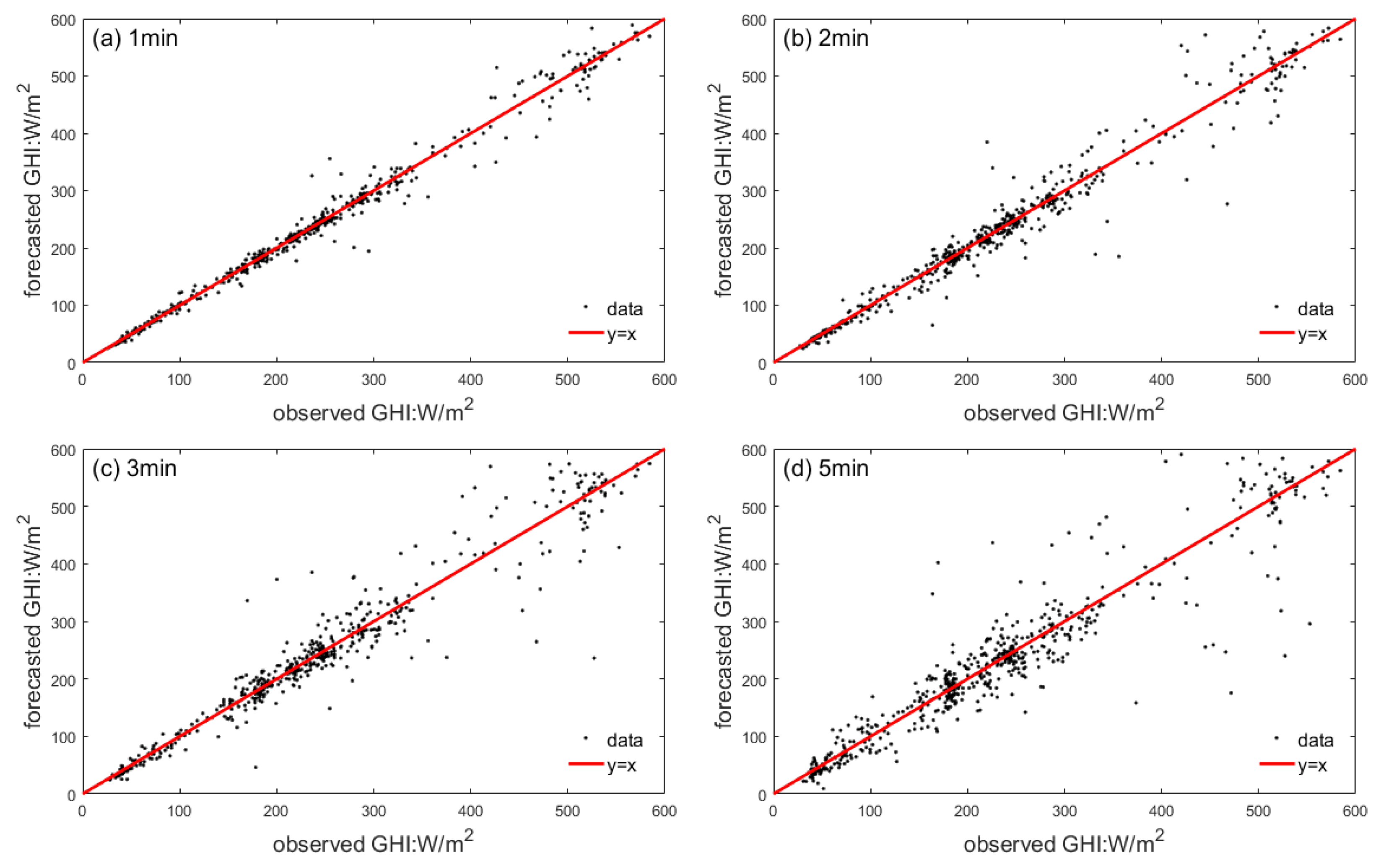
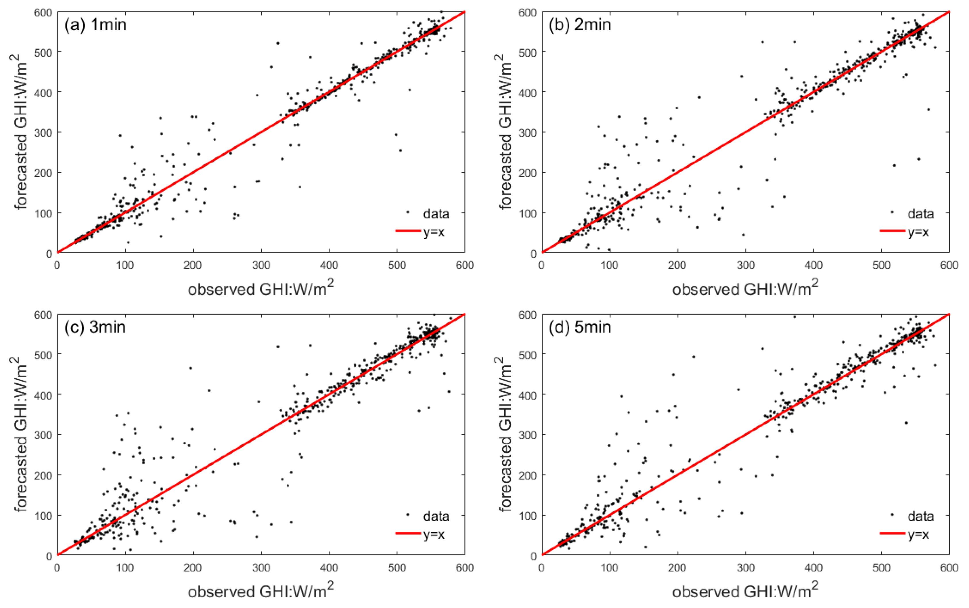
3.4.3. Results of GHI Forecasting

Clear or overcast days will always result in perfect forecasting, making them unsuitable for reflecting the ground irradiance response to changes in cloud fraction and evaluating the performance of forecasting models with the sky imager; hence, these days are eliminated. The 4 representative days with partial clouds were selected from November 2017, including 5th November, 7th November, 8th November, and 11th November.

Although nowcasting of GHI is not affected by the cloud motion, it can be used as a verification method for the accuracy of the cloud detection and the significance of the ternary linear regression equation. Hence, the nowcasting of GHI obtained from formula 5 was used for verifying the rationality of the TLR model in this paper. The results of GHI nowcasting for 5 November 2017 and 7 November 2017 are shown in Figure 9a, and Figure 10a showed that the correlation between forecasted GHI and observed GHI is almost 1, indicating that all the nowcasting GHI can match the observed GHI. Additionally, from Figure 9 and Figure 10b,c, we also found that the forecasted GHI could adequately match the randomness and uncertainty of the observed GHI. In other words, the ternary linear regression equation based on the three different sky types has a significant regression effect, and can consequently be applied for further forecasting.

The scatter diagrams shown in Figure 11 are the result of GHI forecasting ranging from 1 to 5 min on 5 November 2017 and the various errors are given in

Table 1. Forecasting error comparison between the ternary linear regression (TRL) model and the back propagation neural network (BPN) model on 5 November 2017, RMSE: root mean square error, MAE: mean absolute error, MBE: mean bias error; rRMSE: relative root mean square error, rMAE: relative mean absolute error, rMBE: relative mean bias error.

Model	Time Scale	RMSE	MAE	MBE	rRMSE	rMAE	rMBE	R
TLR	0 min	8.593	4.460	0.370	0.038	0.020	0.002	0.998
	1 min	46.732	26.479	0.279	0.203	0.115	0.001	0.95
	2 min	64.119	38.595	−1.107	0.278	0.167	−0.005	0.91
	3 min	83.427	49.840	−4.934	0.347	0.208	−0.021	0.86
	5 min	117.063	71.094	−7.650	0.502	0.305	−0.033	0.83
BPN	1 min	16.070	8.649	−0.971	0.069	0.037	−0.004	0.993
	2 min	27.431	14.760	−1.206	0.118	0.064	−0.005	0.980
	3 min	37.219	21.471	0.017	0.152	0.088	0.000	0.966
	5 min	49.500	28.701	−1.932	0.212	0.123	−0.008	0.936
	10 min	73.136	46.970	−4.762	0.311	0.200	−0.020	0.864

. The points dispersion increases with the increase in time scale, with a validation of r = 0.999, 0.983, 0.967, 0.948 for 1 min, 2 min, 3 min, 5 min, respectively. From Table 1, we also found that the forecasting errors increase with the increase in the forecast time. The various errors during the 4 days were given by Table 1,

Table 2. Forecasting error comparison between the linear regression model and the neural network model on 7 November 2017.

Model	Time Scale	RMSE	MAE	MBE	rRMSE	rMAE	rMBE	R
TLR	0 min	33.320	15.906	2.411	0.117	0.056	0.008	0.996
	1 min	48.784	30.077	1.221	0.169	0.104	0.004	0.931
	2 min	65.655	44.577	0.628	0.227	0.154	0.002	0.882
	3 min	102.039	68.285	−1.546	0.352	0.236	−0.005	0.757
	5 min	124.722	85.332	−3.327	0.429	0.294	−0.011	0.672
BPN	1 min	43.307	26.267	−0.065	0.151	0.092	0.000	0.937
	2 min	56.867	36.142	−2.368	0.198	0.126	−0.008	0.893
	3 min	81.953	54.740	−0.672	0.286	0.191	−0.002	0.801
	5 min	97.350	63.719	4.313	0.338	0.221	0.015	0.742
	10 min	124.594	89.594	2.770	0.430	0.309	0.010	0.555

,

Table 3. Forecasting error comparison between the linear regression model and the neural network model on 8 November 2017.

Model	Time Scale	RMSE	MAE	MBE	rRMSE	rMAE	rMBE	R
TLR	0 min	6.562	1.885	−0.076	0.020	0.006	0.000	0.996
	1 min	32.690	14.152	0.958	0.096	0.042	0.003	0.931
	2 min	54.270	24.522	2.736	0.164	0.074	0.008	0.882
	3 min	49.692	24.503	−4.380	0.149	0.074	−0.013	0.757
	5 min	58.799	30.687	−6.170	0.176	0.092	−0.018	0.672
BPN	1 min	47.604	27.184	0.368	0.173	0.099	0.001	0.944
	2 min	66.083	40.428	−5.953	0.240	0.147	−0.022	0.889
	3 min	81.247	52.912	−4.567	0.294	0.192	−0.017	0.841
	5 min	98.843	65.099	−2.602	0.357	0.235	−0.009	0.773
	10 min	109.479	74.403	−5.503	0.452	0.307	−0.023	0.727

and

Table 4. Forecasting error comparison between the linear regression model and the neural network model on 11 November 2017.

Model	Time Scale	RMSE	MAE	MBE	rRMSE	rMAE	rMBE	R
TLR	0 min	8.579	2.973	−1.494	0.026	0.009	−0.005	0.999
	1 min	31.334	13.912	−4.006	0.092	0.041	−0.012	0.988
	2 min	52.052	22.725	−7.152	0.157	0.068	−0.022	0.967
	3 min	71.395	31.077	−10.971	0.215	0.093	−0.033	0.941
	5 min	111.740	45.512	−21.055	0.335	0.136	−0.063	0.875
BPN	1 min	38.779	18.536	1.195	0.116	0.055	0.004	0.980
	2 min	53.112	26.449	0.922	0.158	0.079	0.003	0.963
	3 min	55.241	27.653	2.119	0.165	0.083	0.006	0.961
	5 min	57.718	30.609	0.817	0.172	0.091	0.002	0.956
	10 min	81.365	50.763	1.780	0.321	0.401	0.010	0.895

. As expected from the previous studies, higher lead times resulted in higher errors. The average RMSE of the 4 selected days for 1 min, 2 min, 3 min, and 5 min forecasting are 39.89 W/m², 59.02 W/m², 76.64 W/m² and 103.08 W/m²; the average rRMSE are 14%, 21%, 27%, 36%, respectively. Bias values (MBE and rMBE) showed negative values, indicating that more sky clear pixels were incorrectly assigned as cloud.

By taking the neural network dynamic rolling learning method, the comparisons between the forecasted and measured GHI on 5 November and 11 November 2017 are given by Figure 12 and Figure 13. The points with larger deviation correspond to the moment when the radiation changes sharply. Bias values (MBE and rMBE) also showing negative values may be related to excessive boundary clouds.

The comparisons of forecasting errors for the 4 days are shown in Table 1, Table 2, Table 3 and Table 4. The 4-day average error is shown in

Table 5. The average forecasting error of 4 days comparison between the linear regression model and the neural network model.

Model	Time Scale	RMSE	MAE	MBE	rRMSE	rMAE	rMBE
TLR	0 min	14.26	6.31	0.30	0.05	0.023	0.001
	1 min	39.89	21.16	−0.39	0.14	0.076	−0.001
	2 min	59.02	32.60	−1.22	0.21	0.116	−0.004
	3 min	76.64	43.43	−5.46	0.27	0.15	−0.018
	5 min	103.08	58.16	−9.55	0.36	0.21	−0.031
BPN	1 min	38.78	18.54	1.20	0.12	0.055	0.004
	2 min	53.11	26.45	0.92	0.16	0.079	0.003
	3 min	55.24	27.65	2.20	0.17	0.083	0.006
	5 min	57.72	30.61	0.82	0.17	0.091	0.002
	10 min	81.37	50.76	1.78	0.32	0.401	0.010

. It is obvious that the errors of RMSE, MAE and MBE of the two kinds of forecasting all increase with the increase in lead time, and the correlation coefficient decreases with the increase in lead time.

Although the cloud fraction and clear sky index satisfy the multiple linear regression relation in a short time (several minutes), when using this linear relation to statistically extrapolate the future irradiance, the forecast performance is not as good as the neural network forecast model and the error is larger. The reason for this is that, under broken sky conditions with rapid changes of cloud fraction and speed, the nonlinear BPN-based model can reflect these changes more effectively. This is because neural networks have the ability to learn and can handle complex non-linear problems.

4. Discussion

The two GHI forecasting models developed in this paper are mainly based on the ground observational characteristics of clouds from the Dunhuang region of China, considering the attenuation effect of clouds with different thickness and proportion on GHI. To apply them to other areas, cloud detection and forecasting technologies are universal and necessary adjustment based on observations for the clear sky model are needed. Meanwhile, the radiation transmission in cloudy atmosphere is an extremely complicated process and the interaction mechanism between radiation and clouds remains poorly understood. In fact, clouds with different heights have diverse attenuation effects on radiation. However, cloud base height is not available for a single TSI site. Unified processing of clouds of different heights is likely to increase the error of forecasting.

Moreover, in this study, the temporal–spatial range is limited by the observation range of the ground sky imager. The boundary information of forecasted cloud images comes from the original images and cannot represent the sky situation in the future. When the clouds move fast, the forecasting error of the cloud image increases and the forecasting time scale reduces.

Overall, the average rRMSE of the 4 selected days ranged from 5% to 36% based on the TLR model and ranged from 12% to 32% based on the BPN model. In the previous study, the forecasting with four all-sky cameras, which were claimed to be state of the art, reduced the rRMSE of GHI from 30.9% to 23.5% [11]; however, the computational efficiency and cost were also much higher.

Dunhuang is located in northwestern China; the weather in winter is usually dry. There is almost no typical synoptic process during the observation period, broken days are few and the optical thickness of cloud is small. On the one hand, thin high-altitude cloud is hard to be accurately detected in the sky images, and the error of cloud detection and retrieval limited the accuracy of irradiance forecasting. On the other hand, thin clouds are prone to move and dissipate quickly, making forecasting more difficult and the time scale smaller.

In view of the shortcomings in the current work, the prospects for future work are proposed: The localized network of TSI observation will be deployed to retrieve the cloud base height and extract the cloud information and join the multiple images from different sites at the same time, achieving the monitoring of cloud motion in a larger area and improving spatial-temporal scale and accuracy of refined forecasting of solar radiation.

5. Conclusions

Two rolling forecasting models of GHI were established in this study based on the observation of a TSI and radiometer at a PV plant in Dunhuang, China. The main technical work included cloud detection and forecasting. To our knowledge, this is first time that such models have been developed and compared. Although the complicated effect of clouds on radiation is simplified in the models, especially in the TLR model, by including the objective observational characteristics of clouds into the surface radiation based on clear sky radiation, we simulated the GHI under the partly cloudy sky conditions. The two models allow us to effectively model the decreasing or increasing trend and degree of local GHI from the deployment of the ground observation of clouds; this is of significant relevance to the scheduling, dispatching and regulation of PV plants’ power.

For cloud detection, the area around the sun and near-horizontal area are difficult to distinguish accurately; the error of thin cloud, especially in the areas around the sun and the shading areas, is greater than thick cloud. The threshold of clear sky and thick cloud is 0.067 and 0.225, respectively, in this study.

The accuracy of cloud map prediction is limited by the accuracy of cloud recognition. Because of the limited view of TSI, there will be clouds moving outside of the image, causing errors in the forecasted cloud map, through advection transport, to increase with the increase in lead time, and causing the average rRMSE of the 4 selected days to range from 5% to 36% based on the TLR model and from 12% to 32% based on the BPN model.

References

1. Haegel, N.M.; Margolis, R.; Buonassisi, T.; Feldman, D.; Froitzheim, A.; Garabedian, R.; Green, M.; Glunz, S.; Henning, H.-M.; Holder, B.; et al. Terawatt-scale photovoltaics: Trajectories and challenges. Science 2017, 356, 141–143. [Google Scholar] [CrossRef] [PubMed]
2. Breyer, C.; Bogdanov, D.; Gulagi, A.; Aghahosseini, A.; Barbosa, L.S.; Koskinen, O.; Barasa, M.; Caldera, U.; Afanasyeva, S.; Child, M.; et al. On the role of solar photovoltaics in global energy transition scenarios. Prog. Photovolt. Res. Appl. 2017, 25, 727–745. [Google Scholar] [CrossRef]
3. Wilson, G.M.; Al-Jassim, M.; Metzger, W.K.; Glunz, S.W.; Verlinden, P.; Xiong, G.; Mansfield, L.M.; Stanbery, B.J.; Zhu, K.; Yan, Y.; et al. The 2020 photovoltaic technologies roadmap. J. Phys. D Appl. Phys. 2020, 53, 493001. [Google Scholar] [CrossRef]
4. IEA. 2020. Available online: https://www.iea.org/reports/solar-pv (accessed on 1 October 2020).
5. Lave, M.; Kleissl, J. Solar variability of four sites across the state of Colorado. Renew. Energy 2010, 35, 2867–2873. [Google Scholar] [CrossRef] [Green Version]
6. Li, F.; Chen, Z.; Cheng, C.; Duan, S. Review on Forecast Methods for Photovoltaic Power Generation. Adv. Clim. Chang. Res. 2011, 7, 136–142. [Google Scholar]
7. Li, W.H.; He, X.N. Review of Nonisolated High-Step-Up DC/DC Converters in Photovoltaic Grid-Connected Applications. IEEE Trans. Ind. Electron. 2011, 58, 1239–1250. [Google Scholar] [CrossRef]
8. Marchesoni-Acland, F.; Alonso-Suarez, R. Intra-day solar irradiation forecast using RLS filters and satellite images. Renew. Energy 2020, 161, 1140–1154. [Google Scholar] [CrossRef]
9. Haupt, S.E.; Dettling, S.; Williams, J.K.; Pearson, J.; Jensen, T.; Brummet, T.; Kosovic, B.; Wiener, G.; McCandless, T.; Burghardt, C. Blending distributed photovoltaic and demand load forecasts. Sol. Energy 2017, 157, 542–551. [Google Scholar] [CrossRef]
10. Zang, H.; Liu, L.; Sun, L.; Cheng, L.; Wei, Z.; Sun, G. Short-term global horizontal irradiance forecasting based on a hybrid CNN-LSTM model with spatiotemporal correlations. Renew. Energy 2020, 160, 26–41. [Google Scholar] [CrossRef]
11. Kuhn, P.; Nouri, B.; Wilbert, S.; Prahl, C.; Kozonek, N.; Schmidt, T.; Yasser, Z.; Ramirez, L.; Zarzalejo, L.; Meyer, A.; et al. Validation of an all-sky imager-based nowcasting system for industrial PV plants. Prog. Photovolt. Res. Appl. 2017, 26, 608–621. [Google Scholar] [CrossRef]
12. Hasenbalg, M.; Kuhn, P.; Wilbert, S.; Nouri, B.; Kazantzidis, A. Benchmarking of six cloud segmentation algorithms for ground-based all-sky imagers. Sol. Energy 2020, 201, 596–614. [Google Scholar] [CrossRef]
13. Yanbo, S.; Zongci, Z.; Guangyu, S. The Progress in Variation of Surface Solar Radiation, Factors and Probable Climatic Effects. Adv. Earth Sci. 2008, 23, 915–923. [Google Scholar]
14. Matuszko, D. Influence of the extent and genera of cloud cover on solar radiation intensity. Int. J. Clim. 2012, 32, 2403–2414. [Google Scholar] [CrossRef]
15. Antonanzas, J.; Osorio, N.; Escobar, R.; Urraca, R.; Martinez-de-Pison, F.J.; Antonanzas-Torres, F. Review of photovoltaic power forecasting. Sol. Energy 2016, 136, 78–111. [Google Scholar] [CrossRef]
16. Pfister, G.; McKenzie, R.L.; Liley, J.B.; Thomas, A.; Forgan, B.W.; Long, C.N. Cloud coverage based on all-sky imaging and its impact on surface solar irradiance. J. Appl. Meteorol. 2003, 42, 1421–1434. [Google Scholar] [CrossRef]
17. Liou, K.-N. Introduction to Atmospheric Radiation; China Meteorological Press: Beijing, China, 2004; p. 494. [Google Scholar]
18. Martin, L.; Zarzalejo, L.F.; Polo, J.; Navarro, A.; Marchante, R.; Cony, M. Prediction of global solar irradiance based on time series analysis: Application to solar thermal power plants energy production planning. Sol. Energy 2010, 84, 1772–1781. [Google Scholar] [CrossRef]
19. Mellit, A.; Eleuch, H.; Benghanem, M.; Elaoun, C.; Pavan, A.M. An adaptive model for predicting of global, direct and diffuse hourly solar irradiance. Energy Conv. Manag. 2010, 51, 771–782. [Google Scholar] [CrossRef]
20. Paoli, C.; Voyant, C.; Muselli, M.; Nivet, M.L. Forecasting of preprocessed daily solar radiation time series using neural networks. Sol. Energy 2010, 84, 2146–2160. [Google Scholar] [CrossRef] [Green Version]
21. Voyant, C.; Muselli, M.; Paoli, C.; Nivet, M.L. Optimization of an artificial neural network dedicated to the multivariate forecasting of daily global radiation. Energy 2011, 36, 348–359. [Google Scholar] [CrossRef] [Green Version]
22. Voyant, C.; Muselli, M.; Paoli, C.; Nivet, M.L. Numerical weather prediction (NWP) and hybrid ARMA/ANN model to predict global radiation. Energy 2012, 39, 341–355. [Google Scholar] [CrossRef] [Green Version]
23. Perez, R.; Lorenz, E.; Pelland, S.; Beauharnois, M.; Van Knowe, G.; Hemker, K.; Heinemann, D.; Remund, J.; Müller, S.C.; Traunmüller, W.; et al. Comparison of numerical weather prediction solar irradiance forecasts in the US, Canada and Europe. Sol. Energy 2013, 94, 305–326. [Google Scholar] [CrossRef]
24. Yagli, G.M.; Yang, D.; Srinivasan, D. Automatic hourly solar forecasting using machine learning models. Renew. Sustain. Energy Rev. 2019, 105, 487–498. [Google Scholar] [CrossRef]
25. Chen, Y.; Zhang, S.; Zhang, W.; Peng, J.; Cai, Y. Multifactor spatio-temporal correlation model based on a combination of convolutional neural network and long short-term memory neural network for wind speed forecasting. Energy Convers. Manag. 2019, 185, 783–799. [Google Scholar] [CrossRef]
26. Lorenz, E.; Hurka, J.; Heinemann, D.; Beyer, H.G. Irradiance Forecasting for the Power Prediction of Grid-Connected Photovoltaic Systems. IEEE J. Sel. Top. Appl. Earth Obs. Remote Sens. 2009, 2, 2–10. [Google Scholar] [CrossRef]
27. Perez, R.; Kivalov, S.; Schlemmer, J.; Hemker, K.; Renne, D.; Hoff, T.E. Validation of short and medium term operational solar radiation forecasts in the US. Sol. Energy 2010, 84, 2161–2172. [Google Scholar] [CrossRef]
28. Mathiesen, P.; Kleissl, J. Evaluation of numerical weather prediction for intra-day solar forecasting in the continental United States. Sol. Energy 2011, 85, 967–977. [Google Scholar] [CrossRef] [Green Version]
29. Calbo, J.; Sabburg, J. Feature extraction from whole-sky ground-based images for cloud-type recognition. J. Atmos. Ocean. Technol. 2008, 25, 3–14. [Google Scholar] [CrossRef] [Green Version]
30. Chow, C.W.; Urquhart, B.; Lave, M.; Dominguez, A.; Kleissl, J.; Shields, J.; Washom, B. Intra-hour forecasting with a total sky imager at the UC San Diego solar energy testbed. Sol. Energy 2011, 85, 2881–2893. [Google Scholar] [CrossRef] [Green Version]
31. Inman, R.H.; Pedro, H.T.C.; Coimbra, C.F.M. Solar forecasting methods for renewable energy integration. Prog. Energy Combust. Sci. 2013, 39, 535–576. [Google Scholar] [CrossRef]
32. Marquez, R.; Coimbra, C.F.M. Intra-hour DNI forecasting based on cloud tracking image analysis. Sol. Energy 2013, 91, 327–336. [Google Scholar] [CrossRef]
33. Quesada-Ruiz, S.; Chu, Y.; Tovar-Pescador, J.; Pedro, H.T.C.; Coimbra, C.F.M. Cloud-tracking methodology for intra-hour DNI forecasting. Sol. Energy 2014, 102, 267–275. [Google Scholar] [CrossRef]
34. Yang, H.D.; Kurtz, B.; Nguyen, D.; Urquhart, B.; Chow, C.W.; Ghonima, M.; Kleissl, J. Solar irradiance forecasting using a ground-based sky imager developed at UC San Diego. Sol. Energy 2014, 103, 502–524. [Google Scholar] [CrossRef]
35. Marquez, R.; Gueorguiev, V.G.; Coimbra, C.F.M. Forecasting of Global Horizontal Irradiance Using Sky Cover Indices. J. Sol. Energy Eng. Trans.-ASME 2013, 135, 5. [Google Scholar] [CrossRef] [Green Version]
36. Chu, Y.H.; Li, M.Y.; Coimbra, C.F.M. Sun-tracking imaging system for intra-hour DNI forecasts. Renew. Energy 2016, 96, 792–799. [Google Scholar] [CrossRef]
37. Du, J.; Min, Q.; Zhang, P.; Guo, J.; Yang, J.; Yin, B. Short-Term Solar Irradiance Forecasts Using Sky Images and Radiative Transfer Model. Energies 2018, 11, 1107. [Google Scholar] [CrossRef] [Green Version]
38. Wang, F.; Xuan, Z.; Zhen, Z.; Li, Y.; Li, K.; Zhao, L.; Shafie-Khah, M.; Catalão, J.P. A minutely solar irradiance forecasting method based on real-time sky image-irradiance mapping model. Energy Convers. Manag. 2020, 220, 113075. [Google Scholar] [CrossRef]
39. Voronych, O.; Höller, R.; Beck, G.L.; Traunmüller, W. Solar PV nowcasting based on skycamera observations. Adv. Sci. Res. 2019, 16, 7–10. [Google Scholar] [CrossRef] [Green Version]
40. Cantor, A. Optics of the atmosphere--Scattering by molecules and particles. IEEE J. Quantum Electron. 1978, 14, 698–699. [Google Scholar] [CrossRef]
41. Schade, N.H.; Macke, A.; Sandmann, H.; Stick, C. Enhanced solar global irradiance during cloudy sky conditions. Meteorol. Z. 2007, 16, 295–303. [Google Scholar] [CrossRef]
42. Huo, J.; Lv, D. A method to retrieve the radiance from all-sky visible images. Acta Meteorol. Sin. 2010, 68, 800–807. [Google Scholar]
43. Han, Y.; Song, J. An equivalent surface model of image distortion and the correction algorithm. Opt. Technol. 2005, 31, 122–124. [Google Scholar]
44. Liou, K.-N. An Introduction to Atmospheric Radiation, 2nd ed.; Academic Press: San Diego, CA, USA, 2004; p. 259. [Google Scholar]
45. Shields, J.E.; Johnson, R.W.; Koehler, T.L. Automated Whole Sky Imaging Systems for Cloud Field Assessment; Fourth Symposium on Global Change Studies: Boston, MA, USA; American Meteorological Society: Boston, MA, USA, 1993; pp. 228–231. [Google Scholar]
46. Mori, N.; Chang, K.A. Introduction to MPIV. Available online: http://www.oceanwave.jp/softwares/mpiv (accessed on 8 October 2020).
47. Chu, Y.H.; Pedro, H.T.C.; Coimbra, C.F.M. Hybrid intra-hour DNI forecasts with sky image processing enhanced by stochastic learning. Sol. Energy 2013, 98, 592–603. [Google Scholar] [CrossRef]
48. Marquez, R.; Pedro, H.T.C.; Coimbra, C.F.M. Hybrid solar forecasting method uses satellite imaging and ground telemetry as inputs to ANNs. Sol. Energy 2013, 92, 176–188. [Google Scholar] [CrossRef]
49. Sheng, P.; Mao, J.; Li, J.; Sang, J.; Pan, N. Atmospheric Physics; China Meteorological Press: Beijing, China, 2006; pp. 84–98. [Google Scholar]
50. Cionco, R.G.; Soon, W.W.-H. Short-term orbital forcing: A quasi-review and a reappraisal of realistic boundary conditions for climate modeling. Earth-Sci. Rev. 2017, 166, 206–222. [Google Scholar] [CrossRef] [Green Version]
51. Ineichen, P. Comparison of eight clear sky broadband models against 16 independent data banks. Sol. Energy 2006, 80, 468–478. [Google Scholar] [CrossRef] [Green Version]
52. Kasten, F.; Czeplak, G. Solar and terrestrial radiation dependent on the amount and type of cloud. Sol. Energy 1980, 24, 177–189. [Google Scholar] [CrossRef]
Figure 1. Appearance and composition of total sky imager (TSI-880).
Remotesensing 12 03671 g001
Figure 2. TSI image: (a) Raw image, (b) occlusion location, (c) occlusion recovery.
Remotesensing 12 03671 g002
Figure 3. Relationship of the scattering angle, zenith angle and azimuthal angle in spherical coordinates (from ref. [44]).
Remotesensing 12 03671 g003
Figure 4. Distribution of RBR (red-blue-ratio) with SPA (Sun-Pixel Angle) and IZA (image zenith angle) in clear sky condition: (a) RBR distribution on 11 August 2015 at SZA = 58° (solar zenith angle); (b) standard deviation of RBR on 4 May, 10 June, 11 August and 24 November 2015 at SZA = 58°.
Remotesensing 12 03671 g004
Figure 5. Probability distribution of three types of pixel RBR difference on sample images.
Remotesensing 12 03671 g005
Figure 6. Process of cloud detection (a) image at 15:10 on 7 May 2015 at SZA = 58°, SAA = 239° (solar azimuth). (b) RBR image. (c) The background RBR image at 15:13 on 7 May 7 at SZA = 58°, SAA = 239°. (d) RBR difference of (b,c). (e) Output of cloud detection. (f) Cloud map corrected by SP (sun parameter) (SP = 0.78), white: thick cloud, gray: thin cloud, blue: clear sky.
Remotesensing 12 03671 g006
Figure 7. Determination of representative velocity vector.
Remotesensing 12 03671 g007
Figure 8. Cloud map forecast and matching error: the forecast cloud map at T + t (c) is produced by advecting the cloud map at time T (b) in the direction of the motion vector computed from (a) (T − 1) and (b) (T). To determine the forecast error (f), the future binary cloud map at time T + t (e) is compared to the forecast binary cloud map (d). Red and green colors in (f) show forecast errors (red: pixel forecast cloudy but actually clear; green: pixel forecast clear but actually cloudy) and white indicates accurate forecasts.
Remotesensing 12 03671 g008
Figure 9. Nowcasting irradiance scatter plots on (a) 5 November 2017, (b) 10:00—12:00 on 5 November 2017, (c) 12:00—14:00 on 5 November 2017, (d) 14:00–16:00 on 5 November 2017.
Remotesensing 12 03671 g009
Figure 10. Nowcasting irradiance scatter plots on (a) 7 November 2017, (b) 10:00—12:00 on 7 November 2017, (c) 12:00—14:00 on 7 November 2017, (d) 14:00—16:00 on 7 November 2017.
Remotesensing 12 03671 g010
Figure 11. Scatter plots of global horizonal irradiance (GHI) forecasting based on ternary linear regression (TRL) model for 1 min (a), 2 min (b), 3 min (c), 5 min (d) on 5 November 2017.
Remotesensing 12 03671 g011
Figure 12. Scatter plots of GHI forecasting based on the BPN model for 1 min (a), 2 min (b), 3 min (c), 5 min (d) on 5 November 2017.
Remotesensing 12 03671 g012
Figure 13. Scatter plots of GHI forecasting based on the BPN model for 1 min (a), 2 min (b), 3 min (c), 5 min (d) on 11 November 2017.
Remotesensing 12 03671 g013