Determination of Cloud Motion Applying the Lucas-Kanade Method to Sky Cam Imagery

Abstract

The atmospheric conditions existing where concentrated solar power plants (CSP) are installed need to be carefully studied. A very important reason for this is because the presence of clouds causes drops in electricity generated from solar energy. Therefore, forecasting the cloud displacement trajectory in real time is one of the functions and tools that CSP operators must develop for plant optimization, and to anticipate drops in solar irradiance. For short forecast of cloud movement (10 min) is enough with describe the cloud advection while for longer forecast (over 15 min), it is necessary to predict both advection and cloud changes. In this paper, we present a model that predict only the cloud advection displacement trajectory for different sky conditions and cloud types at the pixel level, using images obtained from a sky camera, as well as mathematical methods and the Lucas-Kanade method to measure optical flow. In the short term, up to 10 min the future position of the cloud front is predicted with 92% certainty while for 25–30 min, the best predicted precision was 82%.

1. Introduction

The climate of Mexico City is tropical even though the city lies at an altitude of 2250 m above mean sea level [1]. Its geographical location, along with its typical meteorological characteristics, means that convective clouds can develop with warm bases and cold tops, where ice particles form and develop during the early stages of precipitation [2].

Solar energy currently plays an important role in the renewable energy market due to its high conversion into electrical energy through CSP (concentrated solar power) and PV (photovoltaic) plants. The increasing use of solar energy as a source of electricity has led to increased interest in forecasting radiation over short time horizons [3]. In places where it is planned to convert solar energy into electrical energy, it is necessary to forecast the solar irradiance resource for operational optimization. Short-term forecasting is needed for operational planning, switching sources, programming back up and short-term power purchase, as well as planning for reserve usage and peak machine load [3].

CSP plants constantly experience changes in the radiation intensity received because there is a direct relationship between the solar radiation reaching the Earth’s surface and the percentage of cloudiness in the sky (the solar irradiance received is maximum for cloudless skies). In this regard, cloud displacement trajectory forecasting (among other atmospheric conditions) is required in the short to medium term to attenuate the solar radiation intensity, which affects electricity generated from cylindrical-parabolic collectors, central tower plants and other CSP technologies.

When the clouds that cover the sun clear away and this is directly above the CSP, the event can cause receiver instability due to thermal stress; therefore, it is essential to develop a cloud motion detection system to preserve the integrity of the central solar receiver [4].

Furthermore, it is fundamentally important that plant operators can anticipate the amount of solar energy that will be generated in plants so that they can react in advance to future fluctuations in electricity generation. The successful integration of solar electricity from CSP plants into the existing electricity supply requires electricity production forecasting of between 24–48 h to cover the current day and the day ahead [5,6]. Cloud cover has been widely studied in different places around the world, above all to examine the role of clouds in solar radiation measurements [7,8,9,10]. Research studies have applied digitized image analysis to satellite images and sky cameras to study solar radiation estimation and solar radiation attenuation caused by the aerosol column and clouds; this has resulted in estimates with 82% certainty for all sky types [10,11,12,13].

Cloud motion can be determined from sequential pictures obtained from sky cameras and satellite images [14]. Experiments have been conducted using techniques for computing the cloud motion over the time interval between the digitized images. Different techniques have been employed such as directly applying cross-correlation, cross-correlation using the fast Fourier Transform, a relatively simple matching technique used in the computer to recognize binary cloud-field images from each of a pair of images, and optical flow estimation [14,15].

Short and medium-term remote sensing techniques have been used to forecast cloudiness up to 180 min ahead of overcast skies. The methodology is based on determining cloud motion in the images. The short-term forecast (less than 1 h) and the medium-term forecast (up to 3 h) have a success rate of 80% [16]. R. Chauvin and J. Nou have also presented a cloud detection methodology based on a sky-imaging system with RMSE up to 10% [17].

Pekko and Minttu have studied cloud movement by extracting information on cloud cover and cloud movement from ground-based camera images using neural networks and the Lucas-Kanade method. However, thin and transparent clouds were not detected [18]. Similarly, Philip Wood et al. have managed to estimate cloud movement for up to 40 s, segmenting the cloud images according to the difference between the blue and red channels, producing a binary detection image [19]. Regarding cloud movement detection by means of satellite images, Snehlata Shakya employed a fractional-order optical flow method for tracking cloud storms by locating vortexes more accurately [20]. Utilizing satellite images and tools from digital geometry, in combination with an optical flow estimation approach, Hassan Id Ben et al. showed the critical points that can determine which cloud pixel is suitable for tracking its binary skeleton [21]. In tropical regions such as Singapore, where the clouds are mostly formed by convection, Soumyabrata et al. achieved good cloud movement prediction with a lead time of up to 5 min [22]. Juan Du et al. have forecast the global horizontal irradiance for short-term solar irradiance combining the cloud locations on the prediction with a Radiative Transfer Modelusing, the prediction images (up to 10 min ahead) were produced by a non-local optical flow method [23]. Cristian C et al. used the Hans index along with sky images and artificial neural networks to study the percentage of cloud cover; they were able to predict the global horizontal irradiance for one-hour with a 40% error [24].

Likewise, Eric Guilbert and Hui Lin have studied cloud changing (mainly convective clouds) based on the cloud contours model for cloud tracking. They introduced geometric criteria to characterize topological transformations. Geometrical techniques are combined and inserted into a tracking algorithm to perform morphological operations. With their method, they have been able to obtain a history of the cloud positions [25]. Ariana M and Walter R used optical flow and deep learning to extrapolate cloud positions, followed by ray-tracing to predict shadow locations on solar panels and the global horizontal; the results and error metrics were predicted for 15 min ahead [26]. In our case, the research focuses solely on forecasting future cloud positions, or to put it another way, our objective is to determine geometric vectors with cloud displacement while not including internal cloud variations.

The solar energy renewable will continue to be a broad area of study. For this reason, it is necessary to continue improving the solar radiation forecasting models as well as models that forecast cloud motion and cloud changing over time while also considering the correlation that exists between the clouds and their respective shadows on the CSP fields. To continue improving CSP and PV-plant operation, the main topics to investigate are the detection of each movement for all clouds types under different sky conditions and the solar radiation attenuation they cause before reaching the plants.

In this paper we present a model that detects and predicts the cloud advection displacement trajectory for different sky conditions and cloud types (high, medium and low) in real time at the short term. A total sky camera (model TSI-880) was used to carry out this study, which tracked the clouds at the pixel level using the Lucas-Kanade method to measure optical flow.

2. Methodology

2.1. Data

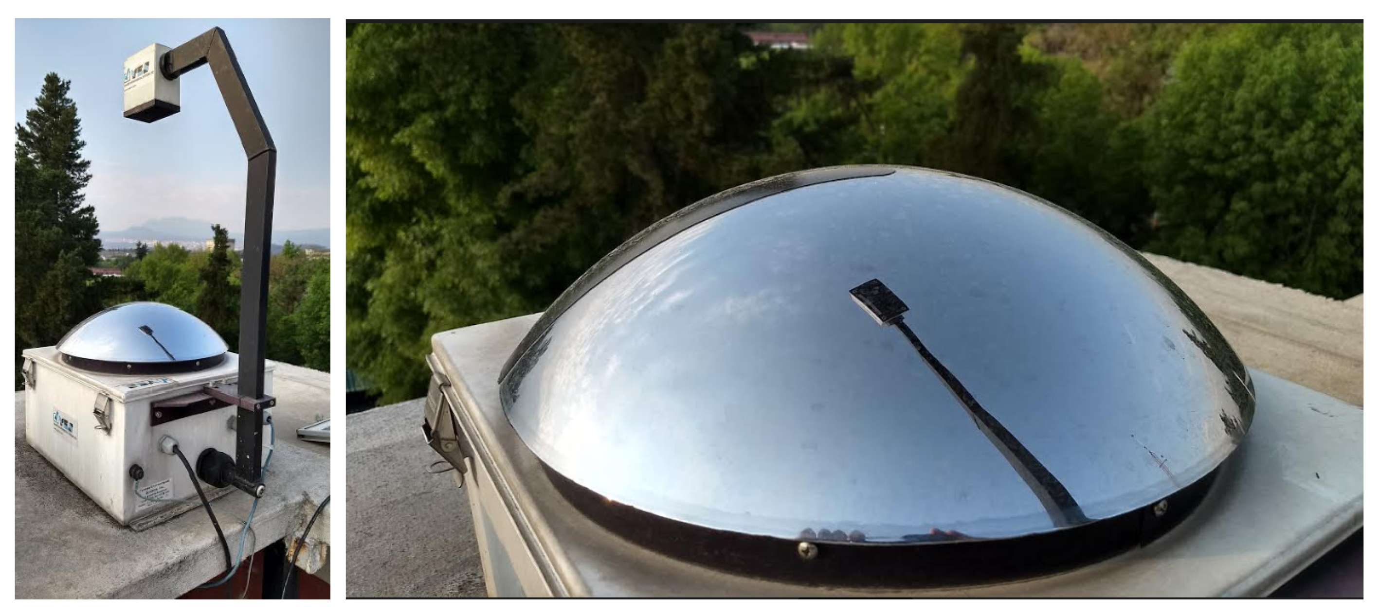
The images used in this work were obtained from the Solar Irradiance Observatory (SIO) at the Geophysics Institute of the National Autonomous University of Mexico (latitude: 19.32, longitude: −99.17, elevation: 2280 m above sea level). The observatory serves as the Regional Center for the Measurement of Solar Irradiance, part of the World Meteorological Organization (WMO).

A total sky camera with a rotational shadow band (the TSI 880 model) Figure 1 providing a hemispheric view of the sky was used to obtain minute-by-minute images from 6:00 a.m. to 6:00 p.m. throughout 2016 and 2017. The hemispheric vision has a 352 × 288-pixel image resolution, represented by 24 bits. The camera’s digitized image is composed of RGB channels [red, green and blue] and HSV [hue, saturation and brightness]. The RGB values range from [0–255] supposing a pixel resolution of 8 bits while the HSVE values range from [0–1].

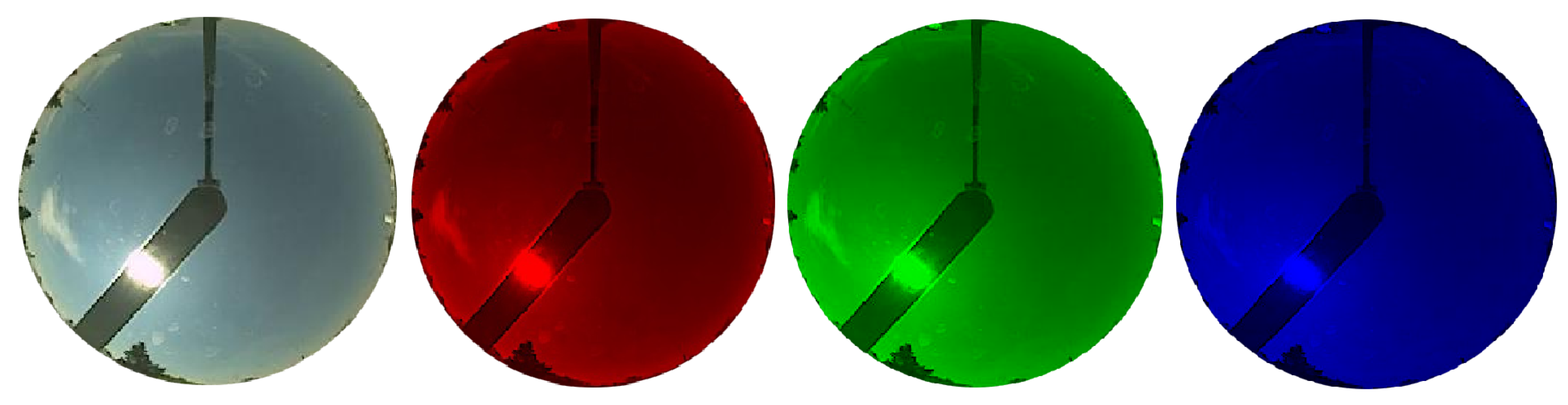
2.2. Cloud Front Motion Detection

The clouds present in the images move from one point to another during defined times of the day, so our objective is to detect those moving clouds and calculate their future position. All cloud types are detectable to the sky camera: low clouds (stratocumulus, cumulus and stratus), medium clouds (altocumulus and altostratus), and high clouds (cirrostratus and cirrus-thin clouds). However, not all types of cloud are easy to track because some are dimmer than others due to the heights at which they are formed. In this paper we perform a methodology that solves the problem of detecting the movement of all cloud types. We start by extracting the image’s red channel, which produces a greater contrast intensity between the clouds and the sky Figure 2.

Later, we subtract two consecutive images successively. At the pixel level, the areas of the image where movement is not recorded have a subtraction value of zero whereas the subtraction value is different from zero where movement is recorded. Using this processing technique, consecutive images were obtained only showing cloud movement. The cloud displacement which follows a defined trajectory is referred to as a cloud front. An example of this method is shown below.

2.3. Cloud Movement Estimation Based on the Lukas-Kanade Method

We employed the Lucas–Kanade method because it is a widely used differential method for optical flow estimation and computer vision. This method solves the basic optical flow equations for all the pixels in the neighborhood using the least squares criterion. It assumes that the flow is essentially constant in the neighborhood around the pixel under consideration [28,29], thus reducing the computational cost. The Lucas-Kanade method detects any rapid change in intensity at the pixel level where there is cloud movement. To track the trajectory of the cloud front displacement, we worked with optic flow using this method and the linear regression mathematical method to predict the future position of the displacement.

The optical flow method calculates the movement between two image frames taken at time t and $t+\delta t$ in the grid space of a pixel. Considering 1 pixel in the first image frame, $I_1(x,y,t)$, which moves a distance of $\delta x$, $\delta y$ over a time $\delta t$, $I_2(x+\delta x,y+\delta y,t+\delta t)$. We know that the images $I_1(x,y,t)$ and $I_2(x+\delta x,y+\delta y,t+\delta t)$ are the same in a very short time of t. Therefore, we can write [28,29,30]:

$$I_1(x,y,t)=I_2(x+\delta x,y+\delta y,t+\delta t)$$

(1)

It can be assumed small local translations constitute the basis of the movement restriction equation as long as $\delta x$, $\delta y$ and $\delta t$ are not too large. Since we have two functions whose similarity we wish to determine, an expansion can be carried out using the first-order Taylor series in Equation (1) obtaining:

The Taylor series for a given value a is defined:

$$\sum _{n=0}^{\infty }\frac{f^n\left(a\right)}{n!}=f\left(a\right)+\frac{f^{\prime }\left(a\right)}{1!}(x-a)+\frac{f^{{}^{\prime \prime }}\left(a\right)}{2!}{(x-a)}^2+\dots$$

(2)

These methods are called differentials, since are based on local approximations of the Taylor series of the image signal; is to say, are use partial differential with respect to spatial and temporal coordinates.

Applying for Equation (1), making an approximation of order 1:

$$I(x,y,t)=I(x,y,t)+\frac{\partial I}{\partial x}dx+\frac{\partial I}{\partial y}dy+\frac{\partial I}{\partial t}dt$$

(3)

Equaling we have:

$$I(x+\delta x,y+\delta y,t+\delta t)=I(x,y,t)+\frac{\partial I}{\partial x}dx+\frac{\partial I}{\partial y}dy+\frac{\partial I}{\partial t}dt$$

(4)

Dividing the differential part of the previous equation by $dt$:

$$\frac{\partial I}{\partial x}\frac{dx}{dt}+\frac{\partial I}{\partial y}\frac{dy}{dt}+\frac{\partial I}{\partial t}\frac{dt}{dt}=0$$

(5)

By definition we know that the change of the position in time is velocity, therefore we obtain $v_x=\frac{dx}{dt}$ and $v_y=\frac{dy}{dt}$ which are the components of the velocity $(x,y)$ of the image or optical flow and $\frac{dt}{dt}=1$. Rewriting the equation we obtain:

$$\frac{\partial I}{\partial x}{v}_x+\frac{\partial I}{\partial y}{v}_y+\frac{\partial I}{\partial t}=0$$

(6)

where $I_x=\frac{\partial I}{\partial x}$, $I_y=\frac{\partial I}{\partial y}$ and $I_t=\frac{\partial I}{\partial t}$ are the image’s intensity differentials. The Equation (6) is called the continuity equation and indicates the conservation of the spatial intensity associated to the image velocity in the pixel (x, y) at time t. Rewriting the equation we obtain:

$$I_x{V}_x+I_y{V}_y+I_t=0$$

(7)

Solving for $-I_t$:

$$I_x{V}_x+I_y{V}_y=-I_t$$

(8)

Mathematically, we know that:

$$\nabla ·\overrightarrow{F}=\frac{\partial F_x}{\partial x}+\frac{\partial F_y}{\partial y}+\frac{\partial F_z}{\partial z}$$

(9)

$$\left[\begin{array}{cc}{V}_x& V_y\end{array}\right]·\left[\begin{array}{c}{I}_x\\ I_y\end{array}\right]=I_x{V}_x+I_y{V}_y$$

(10)

Therefore we can rewrite Equation (8) as follows:

$$\nabla {\overrightarrow{I}}^T·\overrightarrow{V}=-I_t$$

(11)

This is known as the optical flow equation, where $\nabla {\overrightarrow{I}}^T$ is the spatial gradient of intensity and $\overrightarrow{V}=(V_x,V_y)$ is the image velocity or optical flow to pixel $(x,y)$ at time t. The equation contains two unknowns that cannot be solved directly. To find the optical flow, another set of equations is needed.

2.4. Solution Using the Lucas-Kanade Method

The Lucas-Kanade method assumes that the image content displacement between two close instants is small and approximately constant in the neighborhood of a considered point p. Therefore, it can be assumed that the optical flow equation is equal for all the pixels within a window centered on p. The optical motion equation must satisfy for the pixels $q_1,q_2,\dots q_n$ within a window [28,29].

$$\begin{array}{c}\hfill I_x\left(q_1\right)V_x+I_y\left(q_1\right)V_y=-I_t\left(q_1\right)\\ \hfill I_x\left(q_2\right)V_x+I_y\left(q_2\right)V_y=-I_t\left(q_2\right)\\ \hfill .\\ \hfill .\\ \hfill I_x\left(q_n\right)V_x+I_y\left(q_n\right)V_y=-I_t\left(q_n\right)\end{array}$$

(12)

where $I_x\left(q_1\right),I_y\left(q_1\right),$ and $I_t\left(q_n\right)$ are partial differentials of the image I with respect to the position $(x,y)$ and time t evaluated at point $q_i$.

Rewriting this approach in its matrix form:

$$A=\left[\begin{array}{cc}{I}_x\left(q_1\right)& I_y\left(q_1\right)\\ I_x\left(q_2\right)& I_y\left(q_2\right)\\ .\\ .\\ I_x\left(q_n\right)& I_y\left(q_n\right)\end{array}\right];\overrightarrow{\nu }=\left[\begin{array}{c}{V}_x\\ V_y\end{array}\right];b=\left[\begin{array}{c}-I_t\left(q_1\right)\\ -I_t\left(q_2\right)\\ .\\ .\\ -I_t\left(q_n\right)\end{array}\right]$$

(13)

Therefore we obtain:

$$A\overrightarrow{\nu }=b$$

(14)

This system has more equations than unknowns. The Lucas-Kanade method obtains a solution using the least squares criterion and solves a system of $2\times 2$.

From Equation (14), multiplying both sides by the matrix $A^T$ can be written in another form:

$$A^{T}A\overrightarrow{\nu }=A^{T}b$$

(15)

Solving for $\overrightarrow{\nu }$.

$$\overrightarrow{\nu }={\left(A^{T}A\right)}^{-1}{A}^{T}b$$

(16)

Solving Equation (16) in its matrix form, the result for $(V_x,V_y)$ is:

$$\left[\begin{array}{c}{V}_x\\ V_y\end{array}\right]={\left[\begin{array}{cc}\sum _{i=1}^n{I}_x^2{\left(q_i\right)}^2& \sum _{i=1}^n{I}_x{I}_y{\left(q_i\right)}^2\\ \sum _{i=1}^n{I}_x{I}_y{\left(q_i\right)}^2& \sum _{i=1}^n{I}_y^2{\left(q_i\right)}^2\end{array}\right]}^{-1}\left[\begin{array}{c}-\sum _{i=1}^n{I}_x{I}_t{\left(q_i\right)}^2)\\ -\sum _{i=1}^n{I}_y{I}_t{\left(q_i\right)}^2)\end{array}\right]$$

(17)

The central matrix is an inverse matrix and the matrix $A^{T}A$ is often called the structure tensor of the image at a point P.

2.5. Window Weighting

The least-squares solution gives equal importance to all n pixels in the window. In practice, it is generally better to give more weight to pixels that are closer to the center pixel p. For this, the weighted version of the least-squares in Equation (15) is used.

$$A^{T}WA\overrightarrow{\nu }=A^{T}Wb$$

(18)

Solving $\overrightarrow{\nu }$, we can write this equation in another form:

$$\overrightarrow{\nu }={\left(A^{T}WA\right)}^{-1}{A}^{T}Wb$$

(19)

W is a square matrix that contains the weights $W_{ii}=w_i$ that will be assigned to the pixel equation $q_i$. Therefore, we finally obtain:

$$\left[\begin{array}{c}{V}_x\\ V_y\end{array}\right]={\left[\begin{array}{cc}\sum _{i=1}^n{W}_i{I}_x^2{\left(q_i\right)}^2& \sum _{i=1}^n{W}_i{I}_x{I}_y{\left(q_i\right)}^2\\ \sum _{i=1}^n{W}_i{I}_x{I}_y{\left(q_i\right)}^2& \sum _{i=1}^n{W}_i{I}_y^2{\left(q_i\right)}^2\end{array}\right]}^{-1}\left[\begin{array}{c}-\sum _{i=1}^n{W}_i{I}_x{I}_t{\left(q_i\right)}^2)\\ -\sum _{i=1}^n{W}_i{I}_y{I}_t{\left(q_i\right)}^2)\end{array}\right]$$

(20)

2.6. Cloud Motion Tracking

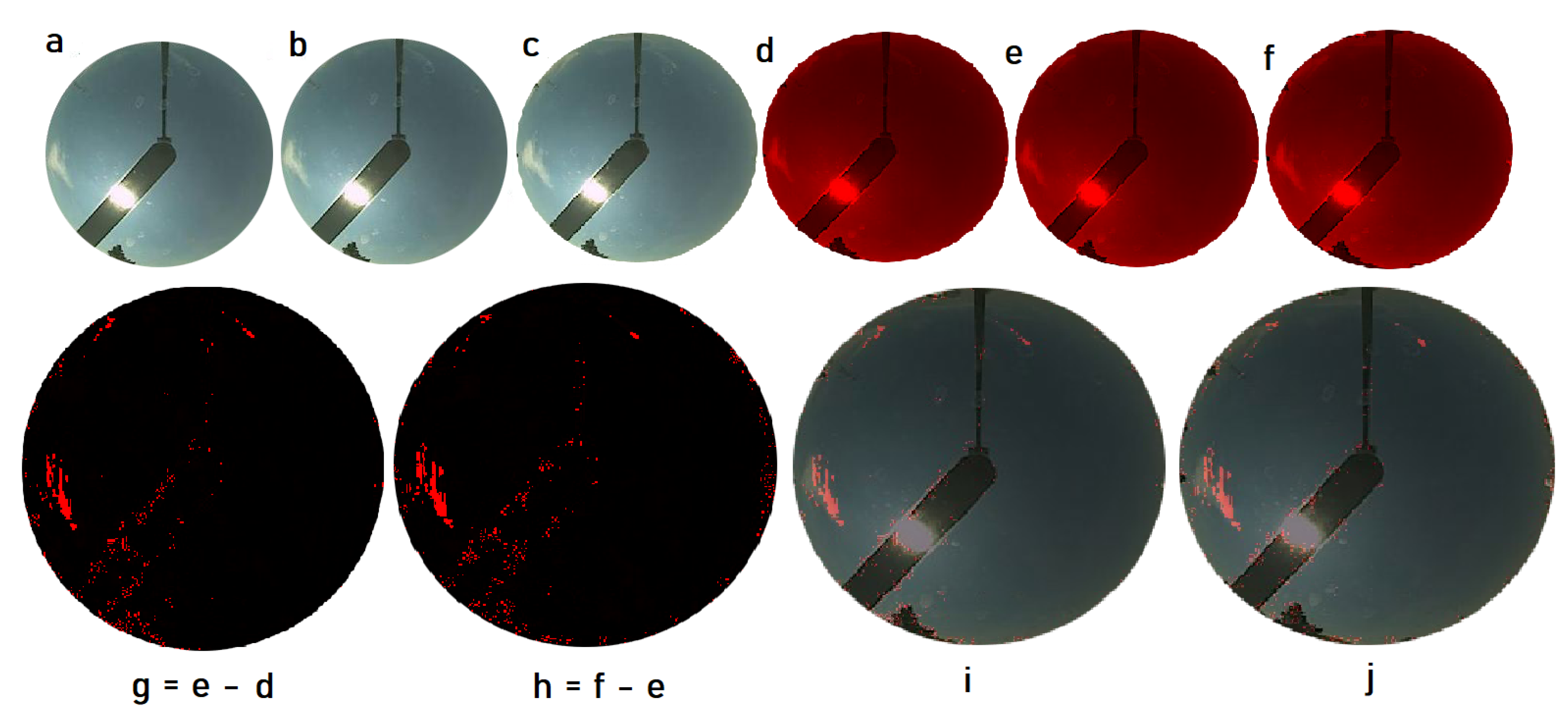
An example of the moving cloud front using the algorithm will be presented in this section. Figure 3a–c correspond to original images and Figure 3d–f are their extracted red channels, respectively. To detect the cloud movement between two consecutive images, we performed the matrix subtraction.

The Figure 3g represents the subtraction between images (e–d) while Figure 3h represents the subtraction between images (f–e). The black color represents the areas of the image where there was no movement detected, while the red color shows the places where there was movement detected between the two consecutive images. Finally, we obtain two consecutive images Figure 3i,j in which the movement of the cloud front is identified and can therefore be tracked. These new images will be used to apply the Lucas-Kanade method.

3. Results

In this section, we present the results for forecasting cloud positions based on their displacement trajectory. To obtain a cloud movement forecast with sufficient time in advance, we used images in which the clouds come from the horizon following a defined trajectory in accordance with the sky camera perspective. Through a developed algorithm, six consecutive images $(i{m}_1,i{m}_2,i{m}_3\dots i{m}_6)$ were subtracted from each other resulting in 5 final images. The subtracted images were denominated in the following form: $I{M}_1=i{m}_2-i{m}_1$, $I{M}_2=i{m}_3-i{m}_2,I{M}_3=i{m}_4-i{m}_3,I{M}_4=i{m}_5-i{m}_4,I{M}_5=i{m}_6-i{m}_5$. Subsequently, we applied the Lucas-Kanade method to $I{M}_1$ with $I{M}_2$, obtaining the displacement vectors of the cloud front. These vectors were averaged in their corresponding vertical and horizontal positions to define a critical point that represents the cloud displacement. To the critical point coordinates $(x_0,y_0)$, we assigned the time $T=0$ min that represented the cloud’s displacement starting point.

Analogously we applied the same procedure to the other images:

• For $T=1$ min of displacement, we applied Lucas-Kanade to $I{M}_2$ with $I{M}_3$, getting $(x_1,y_1)$
• For $T=2$ min of displacement, we applied Lucas-Kanade to $I{M}_3$ with $I{M}_4$, getting $(x_2,y_2)$
• For $T=3$ min of displacement, we applied Lucas-Kanade to $I{M}_4$ with $I{M}_5$, getting $(x_3,y_3)$

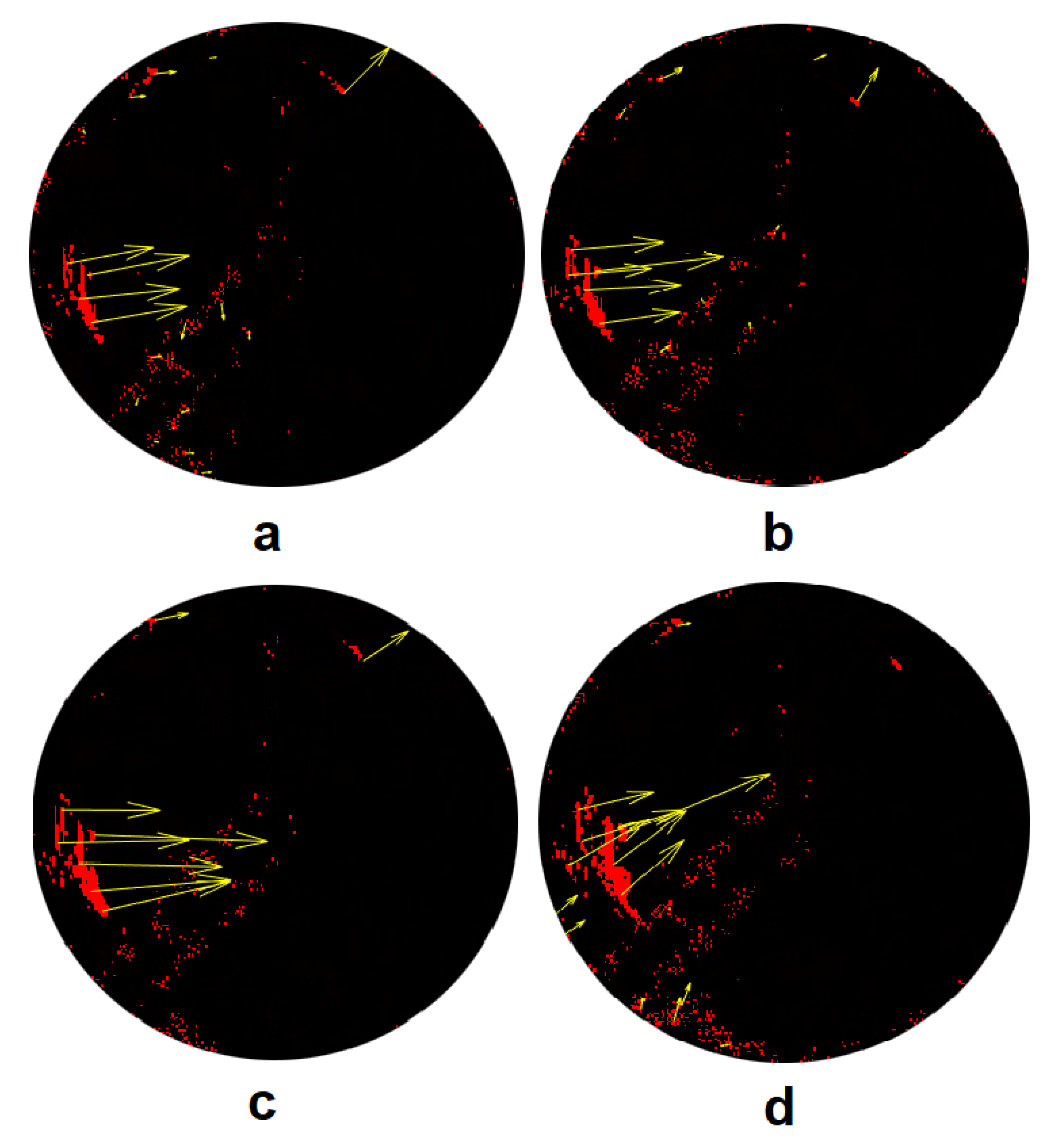
Significantly continuing with the tracking of the cloud front movement identified in Section 2.6. In the Figure 4 shows the cloud front motion detection vectors for times $T=0,1,2,3$ min after applying the Lucas-Kanade method to images $I{M}_{1,2,3,4,5}$. Image $i{m}_1$ corresponds to the image at date 20160219201400, and so on until $i{m}_6=20160219201900$.

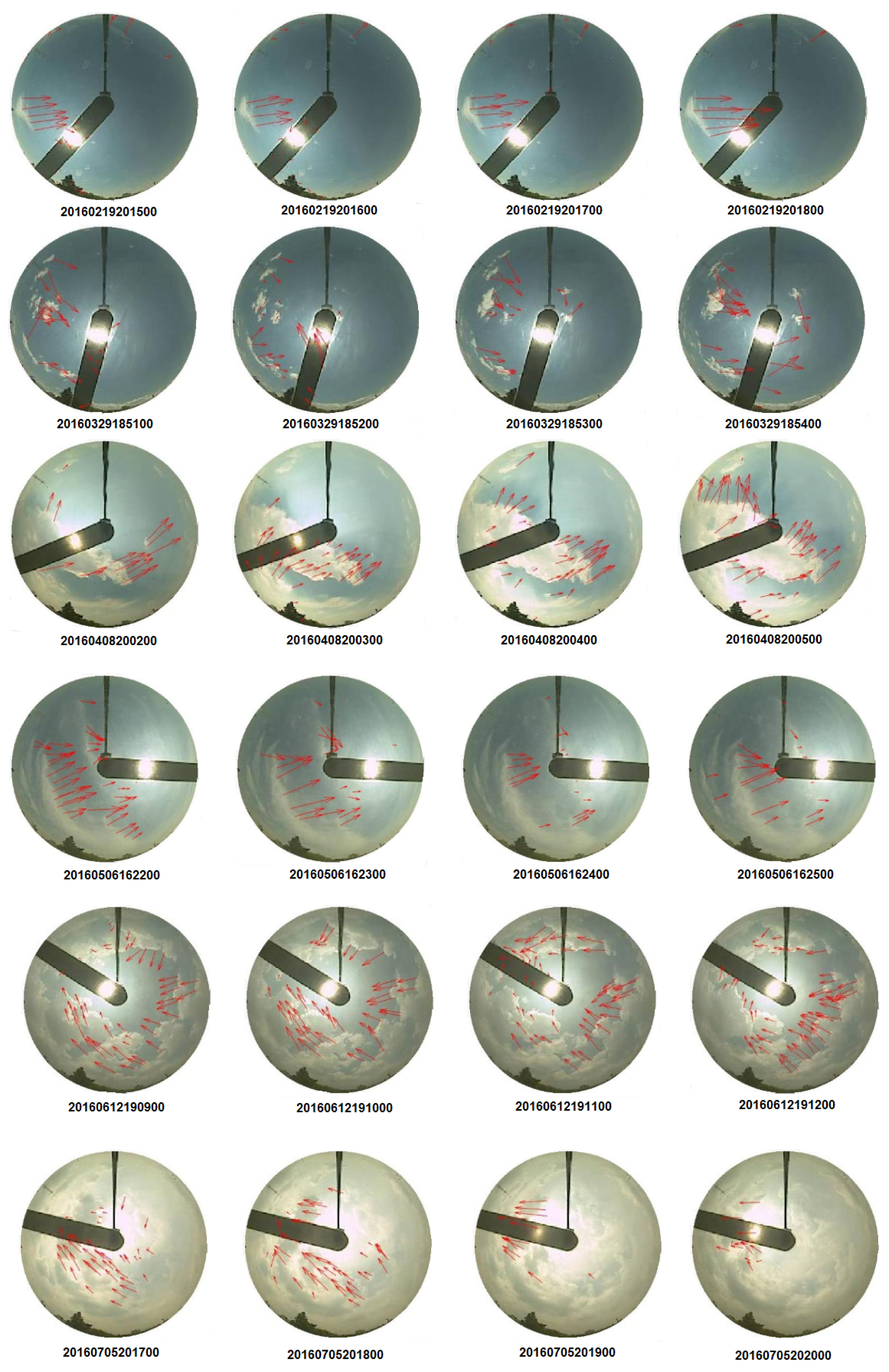
This whole procedure is considered to track the trajectory of a single cloud. The same procedure was performed on fifty cases covering all the seasons of the year and different hours of the day (a total of 500 images were processed). In the Figure 5 presents several cases in which the Lucas-Kanade method was applied.

The developed algorithm was mainly used to analyze partially cloudy skies. If the sky is completely covered by a cloud layer that is similar along its entire length, the algorithm detects only slight cloud transitions. However, if the sky is fully covered and the cloud is not identical in all regions, the algorithm can detect the high motion areas in which the clouds might clear, allowing sunlight to reach the CSP (see Figure 5, 20160705201700-20). These are the moments of interest in terms of the plants being able to continue their operation.

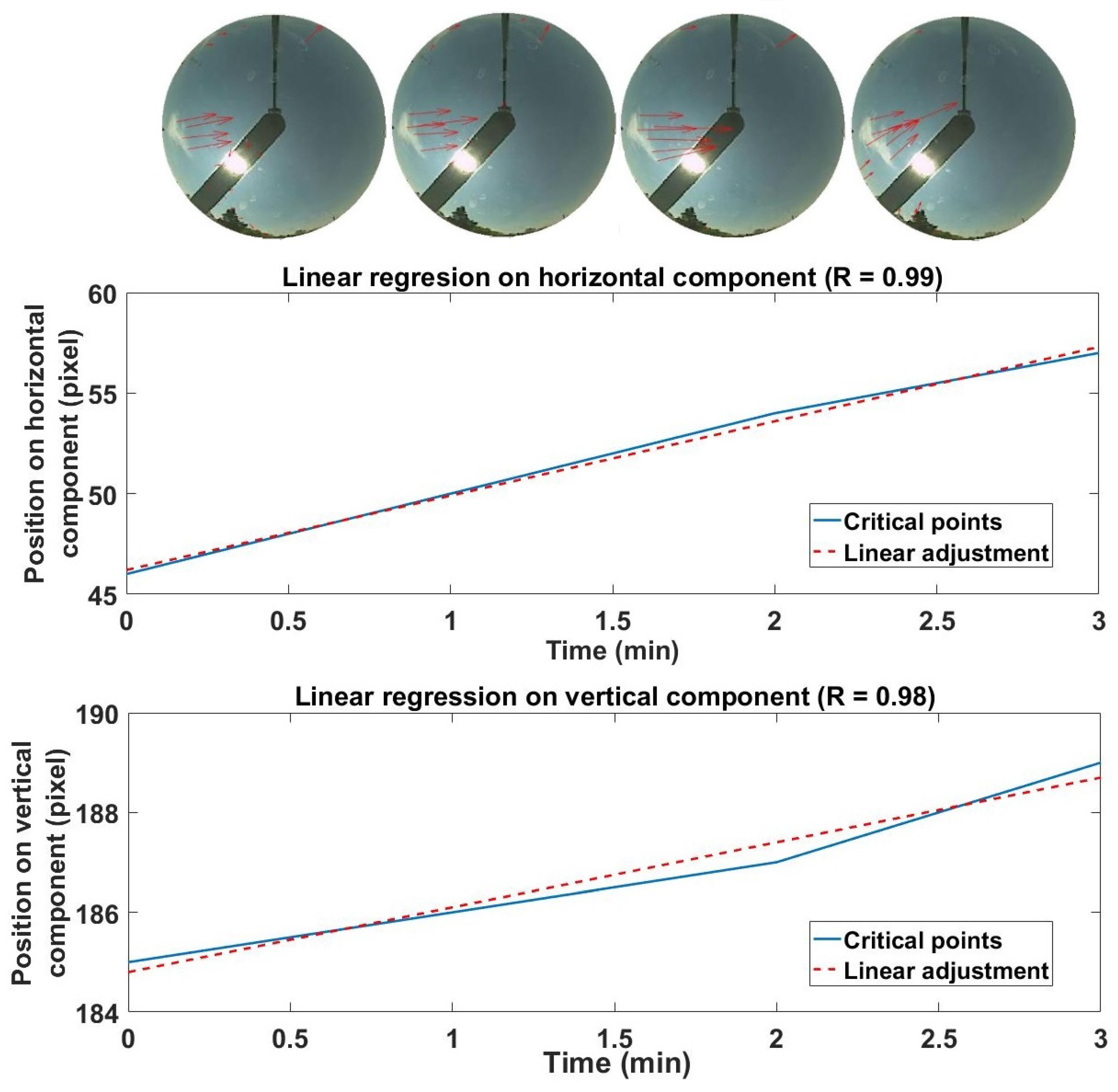
Once the positions $(T,x_T)$ (the displacement trajectory on the horizontal component of the cloud) and $(T,y_T)$ (the displacement trajectory on the vertical component of the cloud) were obtained, we developed a linear regression algorithm and obtained all the displacement functions for $(T=0,1,2,3)$ of the 50 cases analyzed. In the Figure 6 shows the linear regression on the horizontal and vertical components with respect to the cloud front movements identified in Figure 4. The cloud moves from west to east and from north to south (both with positive slopes). The function for the horizontal component is $y=3.7x+46.2$ with an $R=0.99$ and for the vertical component $y=1.3x+184.8$ with an $R=0.98$. This cloud was tracked for a period of 30 min. The statistical results of our methodology are indicated in the table below. The coefficient ratio R of the linear regression was maintained with a certainty above 0.92 for all the cases studied.

Finally, occupying each function, we forecasted the cloud’s displacement trajectory for times subsequent to the image $i{m}_6$. The times that we occupied for the model tests were 2 min, 5 min, 10 min, 15 min, 20 min, 25 min and 30 min.

To validate the results, we occupied the following images up to $i{m}_6$ and analogously located the critical point of the cloud front in Cartesian coordinates at each test time. Subsequently, we calculated the errors using the coordinates forecast by the model.

The indicators proposed for validating the model were:

• Forecast of the critical point on the horizontal component (x)
• Forecast of the critical point on the vertical component (y)
• Forecast of vector magnitude from position at T = 0 to the test time
• Forecast of directionality (angle)

Table 1. Results tracking cloud movement.

Time of	Real Critical Points		Critical Points Forecast		Magnitude Vector (Pixel)			Vector Angle (Directionality) (${}^{\circ }$)
Forecast (min)	X	Y	X	Y	Real	Forecast	Error (%)	Real	Forecast	Error (%)
2	65	191	65	191	20	20	0	17.5	17.5	0.0
5	77	196	76	195	33	32	4	18.4	19.5	1.1
10	100	200	94	202	56	51	9	19.5	15.5	4.0
15	132	216	113	208	91	71	23	18.9	19.8	0.9
20	163	210	131	215	120	90	25	19.4	12.1	7.4
25	190	210	150	221	146	110	25	19.1	9.8	9.2
30	217	200	168	228	172	129	25	19.0	5.0	14

displays the predicted critical points and the critical points of the cloud front for each test time being it practically the same up to 10 min. The results of the magnitude of the vector it are shown together with the angle of displacement of the cloud achieving a certainty of $93\%$ in the cloud directionality up to 20 min. In the Figure 7 shows the cloud in its initial position and the same cloud after 20 min of movement. The yellow line indicates the cloud’s real position, the red line indicates the predicted position and the green line represents the error (an error of 25% in the magnitude vector; see Table 1).

4. Statistical Results

During the displacement, the clouds underwent deformation; therefore, there were cases in which the clouds disappeared, joined with other clouds or accumulated on the image horizon. Cases in which the cloud movements detected by the sky camera could be tracked for more than 30 min were very scarce. For this reason, our analysis considers a test time up to 30 min. The

Table 2. Time total of the clouds in movement.

Time of Forecast (min)	Total Cases	Percentage of Total Cases (%)
2	50	100
5	50	100
10	26	56
15	13	26
20	8	16
25	3	6
30	1	2

displays the time and the total number of cases where the clouds kept moving. In $100\%$ of cases, the cloud front could be tracked during the first 2 and 5 min. In $56\%$ of cases, the clouds maintained their trajectory for 10 min. In $26\%$ of cases, the clouds maintained their trajectory for 15 min. In $16\%$ of cases, the clouds continued on their trajectory for 20 min. In $6\%$ and $2\%$ of cases, the clouds kept moving in the images for up to 25 min and 30 min, respectively.

In the

Table 3. Results tracking cloud movement for all cases.

Time of	Total	Average Error of Vector Magnitude		Average Error	Average Error Angle
Forecast (min)	Cases	Horizontal Component (%)	Vertical Component (%)	Vector Magnitude (%)	(Directionality) (%)
2	50	0.4	0.5	1.4	1.0
5	50	2.1	1.7	4.4	1.8
10	26	7.1	2.5	8.1	2.8
15	13	11.3	3.1	13.9	2.9
20	8	19.2	4.5	16.4	3.8
25	3	11.5	6.6	18.4	5.6
30	1	22.6	12.3	25	14

displays the average error of the magnitude vector forecasting for the horizontal and vertical components of the cloud for all the test times as well as the average angle error. The results show that for the first 5 min the forecast presented a maximum error of $2.1\%$ on the horizontal component, x; for 10 min, the maximum error was $7.1\%$ while for 15 min, it was $11.3\%$. For 20 min the maximum error on the horizontal component, x, was $19.2\%$; for 25 min and 30 min, it remained between $11.5\%$ and $22.6\%$, respectively. We observed that the cloud displacement was similar to the direction of the winds in the study area (southwest, west-oest and northwest) all year round; thus, the greatest displacement occurred over the horizontal component of the cloud, in this sense the minimum error of the prediction is on the vertical component of the cloud displacement.

In terms of directionality, the results show for the first 5 min an error magnitude between the calculated and forecast vector of $4.4\%$, with a directionality error (the error between the angle of the calculated and forecast vector) of $1.8\%$. For the next ten min, the error obtained was $8.1\%$ with a directionality error of $2.8\%$. For 20 min and 25 min, the error remained between $16.4\%$ and $18.4\%$, with a directionality error of $2.9\%$ and $3.8\%$ respectively. For 30 min, the magnitude error was $25\%$ and the directionality error was $14\%$. As the cloud moves away from the initial point, the forecast error increases; however, the model allows forecast the cloud trajectory for up to 30 min of displacement.

The window size that most effectively recognized cloud movement in the Lucas-Kanade algorithm was 60 × 60 pixels. Smaller dimensions recognized movements in less quantity while increasing the size of the window also increased the detection of movement; however, for dimensions bigger that 60x60 pixels, the movement detection again decreased.

5. Conclusions

In this work, we present a model that allows to detect and forecast the cloud advection displacement trajectory for different sky conditions and cloud types under different sky conditions in real time not including the analysis of the cloud’s own transformation. We selected clouds that kept moving for the longest time in the images. In the short term (up to 10 min), the future position of the cloud front was predicted with a certainty of 92% while for (25–30 min), the best precision predicted was 82% with respect to the vector magnitude. Therefore, our work serves to anticipate drops in solar radiation. The study complements a previous work that determined the attenuation factor of direct normal irradiance caused by different cloud types at the pixel level.

Our methodology, which implements the Lucas-Kanade method, allows one to detect the direction of movement of low, medium and high clouds. Low stratocumulus, cumulus and stratus clouds remain more frequently throughout the year. From the images, these clouds can be detected by their appearance on the farthest horizons photographed by the sky camera. These clouds attenuate in an increased amount the solar radiation therefore using this methodology we can determine their trajectory with sufficient reaction time to assist CSP operators.

Middle clouds of the altocumulus and altostratus type move at rates similar to those of low clouds although they begin to be visibly noticed as they get closer to the center of the image.

With respect to high clouds of the cirrostratus and cirrus type (thin clouds), our method is able to identify them and track their trajectory. Unlike low and medium clouds, they maintain their displacement for less time. In addition, their presence is less frequent and, like middle clouds, begin to be visibly noticeable as they approach the center of the image.

This study complements another study which, together, aim to estimate direct solar radiation for solar energy concentration fields. Indeed, by combining the two studies, the conditions for doing so are met with this research. Accordingly, it is possible to forecast the trajectory of the cloud displacement and to determine the direct solar radiation attenuation caused by the clouds. Consequently, this approach provides a tool that allows one to forecast direct radiation in real time.

References

- Ernesto Jauregui, O. El clima de la Ciudad de México. Temas Selectos de Geografía de México 2000, 1, 131. [Google Scholar]
- Montero, G.; Zarraluqui, V.; Caetano, E.; García, F. Hydrometeor vertical characterization of precipitating clouds over the Mexico Basin. Int. J. Remote. Sens. 2011, 32, 6367–6378. [Google Scholar] [CrossRef]
- Reikard, G. Predicing solar radiation at high resolutions: A comparison of time series forecasts. Sol. Energy 2009, 83, 342–349. [Google Scholar] [CrossRef]
- López-Martínez, M.; Rubio, F.R. Cloud Detection System for a Solar Power Tower Plant. In Proceedings of the IEEE 2002 28th Annual Conference of the Industrial Electronics Society, IECON 02, Sevilla, Spain, 5–8 November 2002; pp. 2560–2565. [Google Scholar]
- Mellit, A.; Pavan, A.M. A 24-h forecast of solar irradiance using artificial neural network: Application for performance prediction of a grid-connected PV plant at Trieste, Italy. Sol. Energy 2010, 84, 807–821. [Google Scholar] [CrossRef]
- Schroedter-Homscheid, M.; Gesell, G. Verification os Sectoral Cloud Motion Based Direct Normal Irradiance Nowcasting from Satellite Imagery. AIP Conf. Proc. 2016, 1734, 150007. [Google Scholar] [CrossRef]
- Alonso, J.; Ternero, A.; Batlles, F.J.; Lopez, G.; Rodríguez, J.; Burgaleta, J.I. Prediction of cloudiness in short time periods using techniques of remote sensing and image processing. Energy Procedia 2013, 49, 2280–2289. [Google Scholar] [CrossRef][Green Version]
- Batlles, F.J.; Alonso, J.; López, G. Cloud cver forecasting from METEOSAT data. Energy Procedia 2014, 57, 1317–1326. [Google Scholar] [CrossRef]
- Furlan, C.; de Oliveira, A.P.; Soares, J.; Codato, G.; Escobedo, J.F. The role of clouds in improving the regression model for hourly values of diffuse solar radiation. Appl. Energy 2012, 92, 240–254. [Google Scholar] [CrossRef]
- Alonso-Montesinos, J.; Batles, F. The use of sky camera for solar radiation estimation based on digital image processing. Energy 2015, 90, 377–386. [Google Scholar] [CrossRef]
- Alonso-Montesinos, J.; Batlles, F.; Portillo, C. Solar irradiance forecasting at one-minute intervals for different sky conditions using sky camera images. Energy Convers. Manag. 2015, 105, 1166–1177. [Google Scholar] [CrossRef]
- Alonso-Montesinos, J.; Batles, F.; López, G.; Ternero, A. Sky camera imagery processing based on a sky classification using radiometric data. Energy 2014, 68, 599–608. [Google Scholar] [CrossRef]
- Mondragón, R.; Alonso-Montesinos, J.; Riveros, D.; Valdes, M.; Estevez, H.; Gonzalez-Cabrera, A.E.; Stremme, W. Attenuation Factor Estimation of Direct Normal Irradiance Combining Sky Camera Images and Mathematical Models in an Inter-Tropical Area. Remote Sens. 2020, 12, 1212. [Google Scholar] [CrossRef]
- Leese, J.A.; Novak, C.S.; Taylor, V.R. The Determination of CLoud Pattern Motions from Geosynchronous Satellite Image Data. Pattern Recognit. 1970, 2, 279–292. [Google Scholar] [CrossRef]
- Chauvin, R.; Nou, J.; Thil, S.; Grieu, S. Cloud motion estimation using a sky imager. AIP Conf. Proc. 2015, 1734, 150003. [Google Scholar] [CrossRef]
- Alonso-Montesinos, J.; Batlles, F. Short and medium-term cloudiness forecasting using remote sensing techniques and sky camera imagery. Energy 2014, 73, 890–897. [Google Scholar] [CrossRef]
- Chauvin, R.; Nou, J.; Thil, S.; Traoré, A.; Grieu, S. Cloud detection methodology based on a sky-imaging system. Energy Procedia 2015, 69, 1970–1980. [Google Scholar] [CrossRef]
- Tuominen, P.; Tuononen, M. Cloud Detection and Movement Estimation Based on Sky Camera Images Using Neural Networks and the Lucas- Kanade Method. AIP Conf. Proc. 2017, 1850, 140020. [Google Scholar] [CrossRef]
- Wood-Bradley, P.; Zapata, J.; Pye, J. Cloud Tracking with Optical Flow for Short-Term Solar Forecasting; Solar Thermal Group, Australian National University: Canberra, Australija, 2012. [Google Scholar]
- Shakya, S.; Kumar, S. Characterising and predicting the movement of clouds using fractional-order optical flow. IET Image Process 2019, 13, 1375–1381. [Google Scholar] [CrossRef]
- Idder, H.I.B.; Laachfoubi, N. Cloud Motion Estimation in Satellite Image Sequences by Tracking Skeleton Critical Points using Lucas-Kanade method. In Proceedings of the 13th International Conference Computer Graphics, Imaging and Visualization, Beni Mellal, Morocco, 29 March–1 April 2016; pp. 178–183. [Google Scholar] [CrossRef]
- Dev, S.; Savoy, F.M.; Lee, Y.H.; Winkler, S. Short-Term Prediction of Localized Cloud Motion Using Ground-Based sky Imagers. In Proceedings of the 2016 IEEE Region 10 Conference (TENCON), Singapore, 22–25 November 2016; pp. 2563–2566. [Google Scholar]
- Du, J.; Min, Q.; Zhang, P.; Guo, J.; Yang, J.; Yin, B. Short-Term Solar Irradiance Forecasts Using Sky Images and Radiative Transfer Model. Energies 2018, 11, 1107. [Google Scholar] [CrossRef]
- Crisosto, C.; Hofmann, M.; Mubarak, R.; Seckmeyer, G. One-Hour Prediction of the Global Solar Irradiance from All-Sky Images Using Artificial Neural Networks. Energies 2018, 11, 2906. [Google Scholar] [CrossRef]
- Guilbert, E.; Lin, H. A New Model for Cloud Tracking and Analysis on Satellite Images. Geoinformatica 2007, 11, 287–309. [Google Scholar] [CrossRef]
- Moncada, A.; Richardson, W.; Vega-Avila, R. Deep Learning to Forecast Solar Irradiance Using a Six-Month UTSA SkyImager Dataset. Energies 2018, 11, 1988. [Google Scholar] [CrossRef]
- Escrig, H.; Batles, F.J.; Alonso, J.; Baena, F.M.; Bosch, J.L.; Salbidegoitia, I.B.; Burgaleta, J.I. Cloud detection, classification and motion estimation using geostationary satellite imagery for cloud cover forecast. Energy 2013, 55, 853–859. [Google Scholar] [CrossRef]
- Lucas, B.D.; Kanade, T. An Iterative Image Registration Technique with an Application to Stereo Vision. In Proceedings of the 7th International Joint Conference on Artificial Intelligence (IJCAI), Vancouver, BC, Canada, 24–28 August 1981; Volume 2, pp. 674–679. [Google Scholar]
- Patel, D.; Upadhyay, S. Optical Flow Measurement using et al. Method. Int. J. Comput. Appl. 2013, 61, 5. [Google Scholar]
- Lucas, B.D. Image Matching by the Method of Differences; Carnegie Mellon University: Pittsburgh, PA, USA, 1984. [Google Scholar]
© 2020 by the authors. Licensee MDPI, Basel, Switzerland. This article is an open access article distributed under the terms and conditions of the Creative Commons Attribution (CC BY) license (http://creativecommons.org/licenses/by/4.0/).