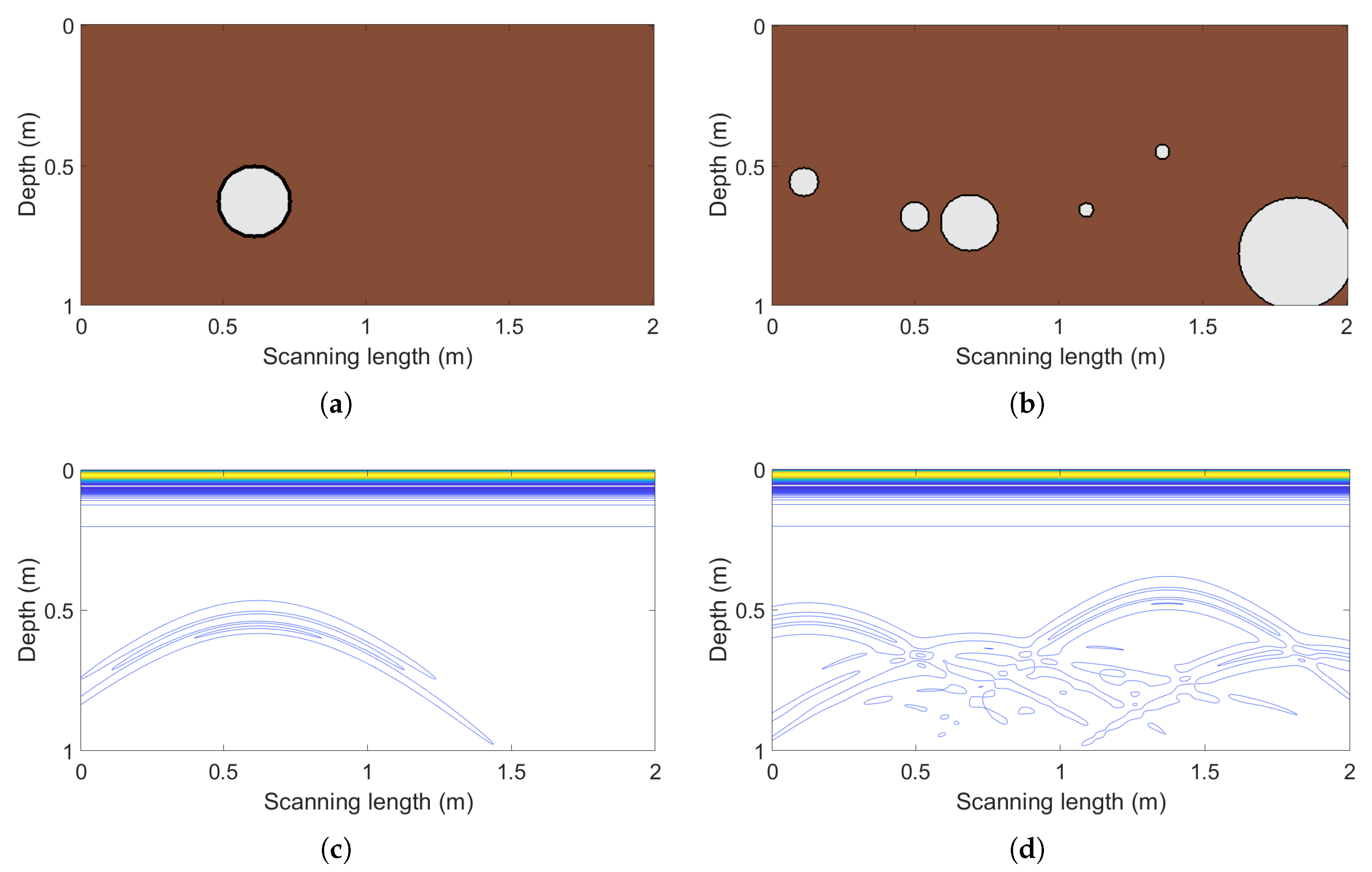
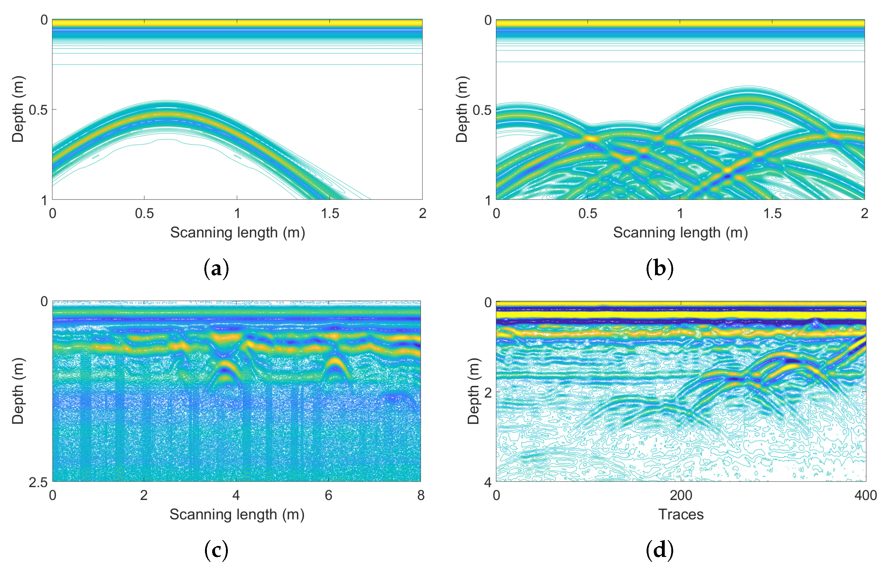
Figure 1.
(a) Example subsurface section with only one pre-buried pipeline, where the brown color represents the soil and the white color represents the pipeline. (b) Example subsurface section with multiple pre-buried pipelines. (c) GPR signal profile corresponding to the subsurface section in panel (a). (d) GPR signal profile corresponding to the subsurface section in panel (b).
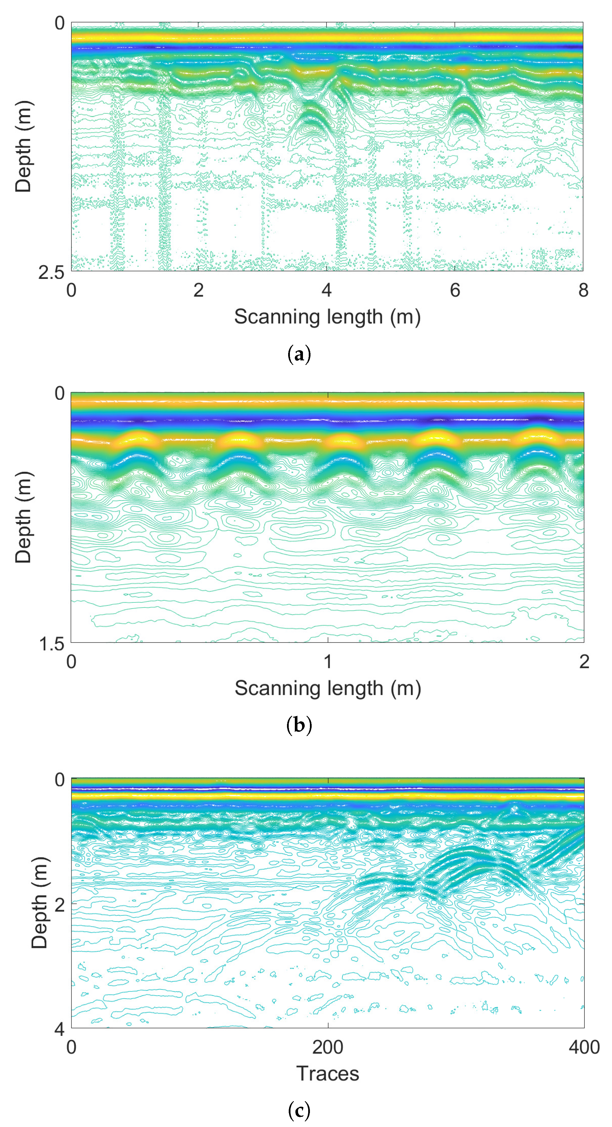
Figure 2.
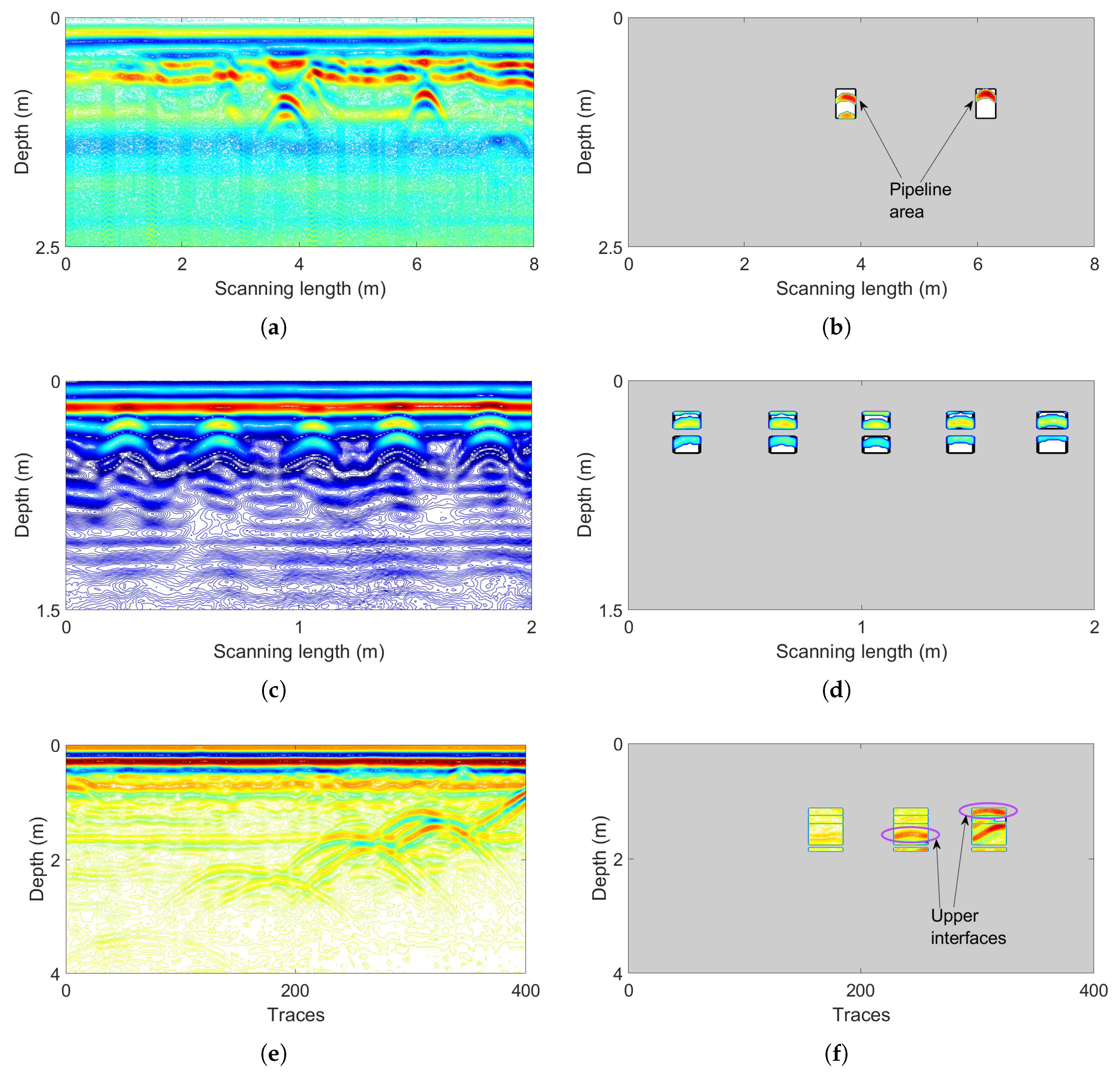
Field GPR profiles of (
a) two separate pre-buried pipelines, (
b) double-layer concrete cylinders, and (
c) three distributed pipelines [
28].
Figure 2.
Field GPR profiles of (
a) two separate pre-buried pipelines, (
b) double-layer concrete cylinders, and (
c) three distributed pipelines [
28].
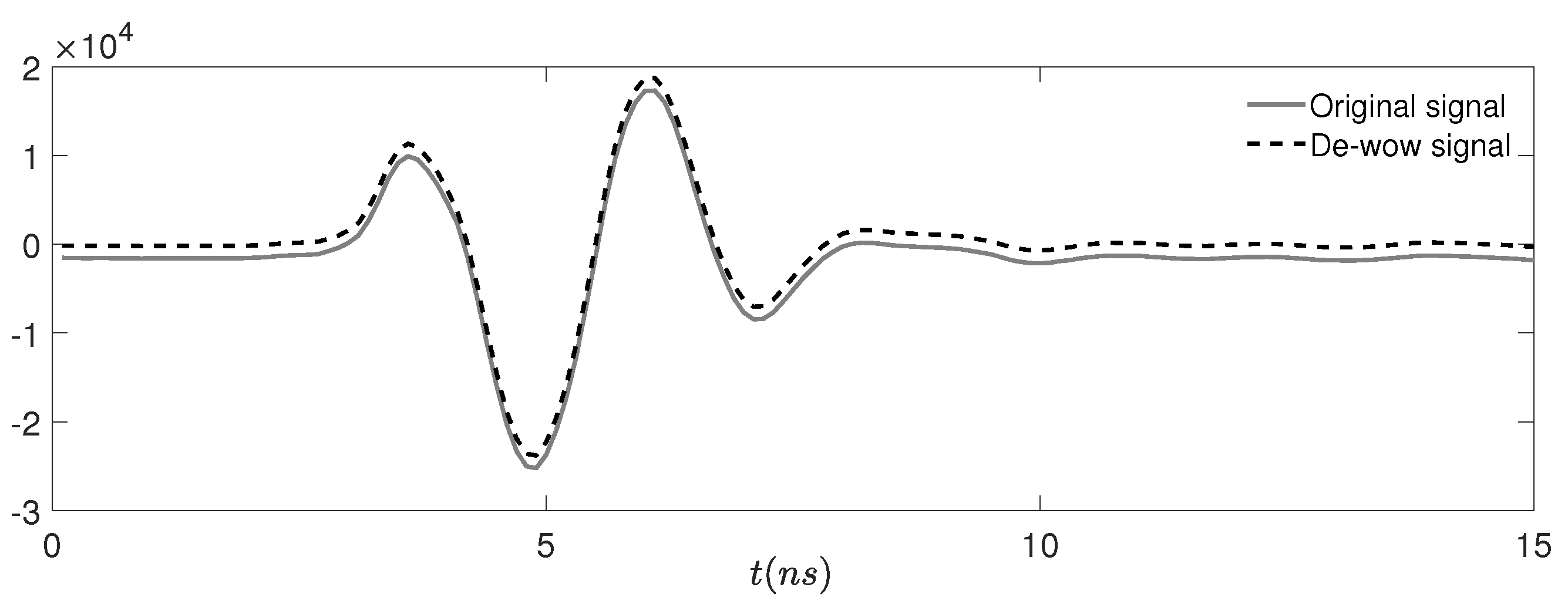
Figure 3.
De-“wow” results of a representative GPR trace.
Figure 3.
De-“wow” results of a representative GPR trace.
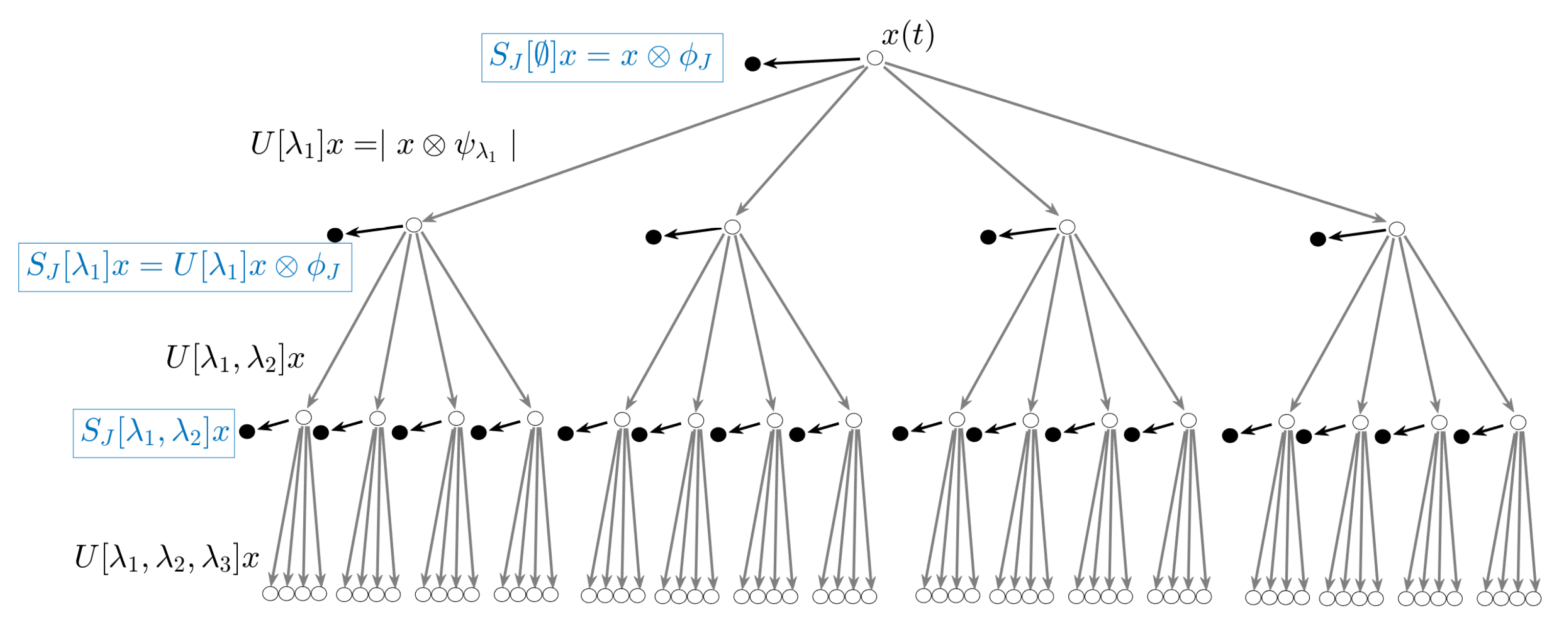
Figure 5.
A three layer wavelet scattering network. The operator is applied to the original signal x to calculate each and output , where ∅ represents an empty set. Then, the operator is applied to each previous layer to calculate all and output . This scattering process is operated iteratively to obtain all convolution results.
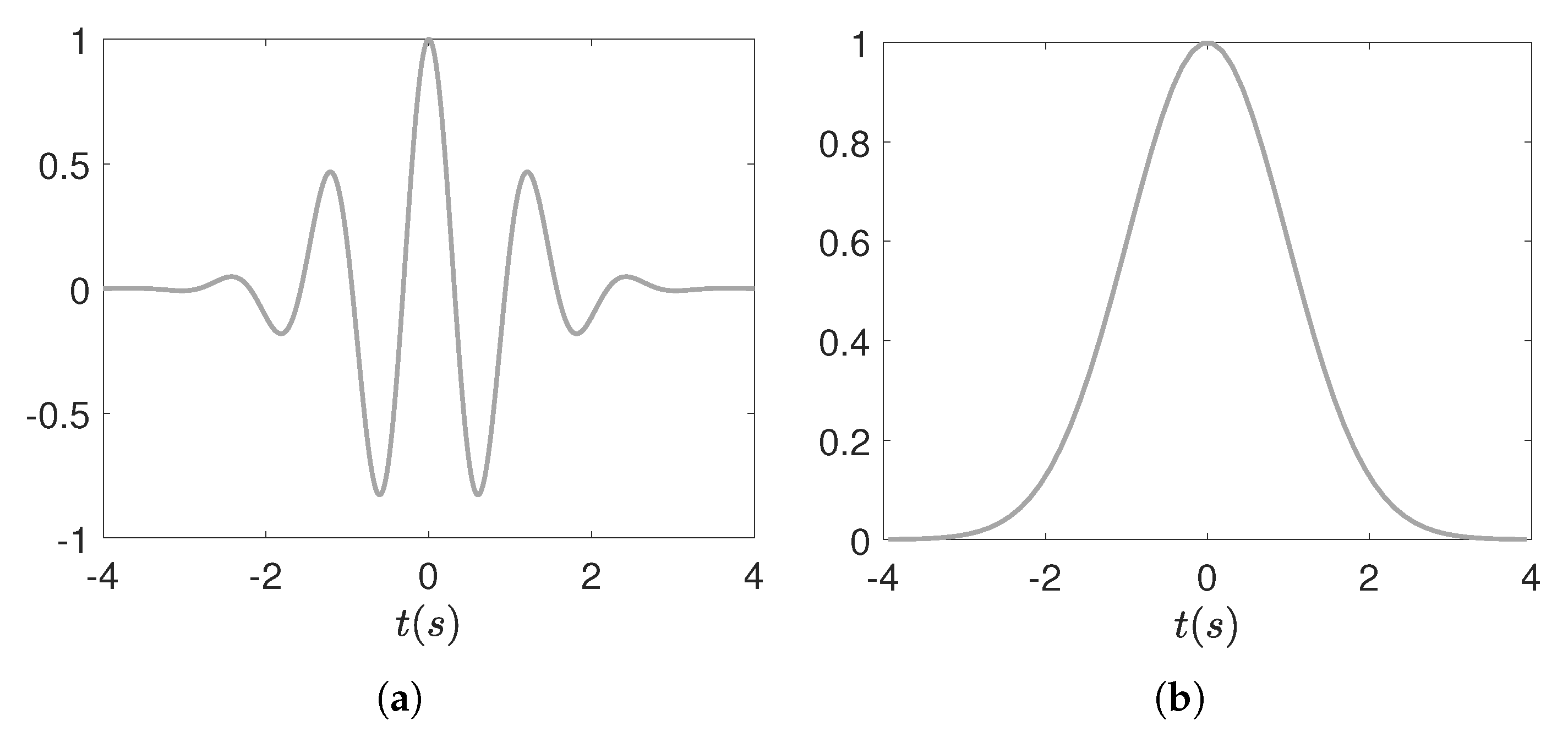
Figure 6.
(a) Real component of example Morlet wavelet with parameters , , and . (b) Example Gaussian window as scale function .
Figure 6.
(a) Real component of example Morlet wavelet with parameters , , and . (b) Example Gaussian window as scale function .
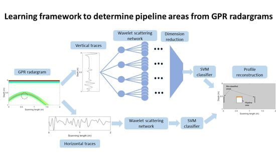
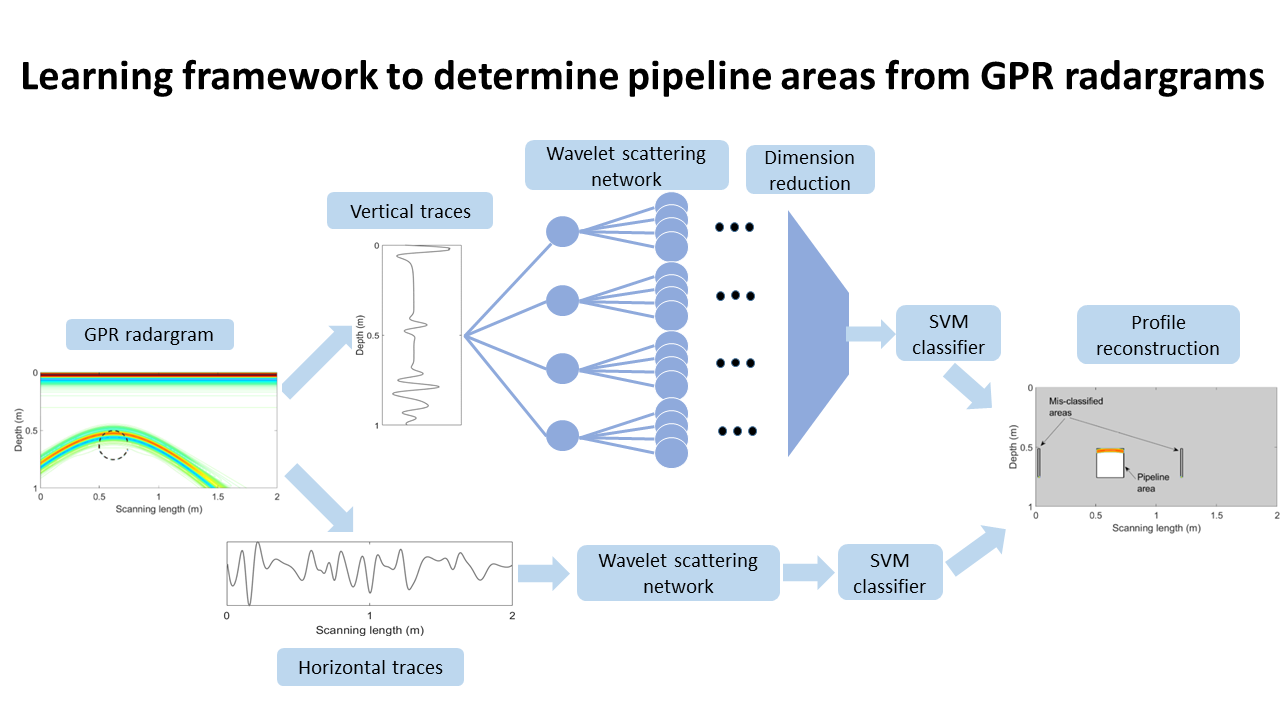
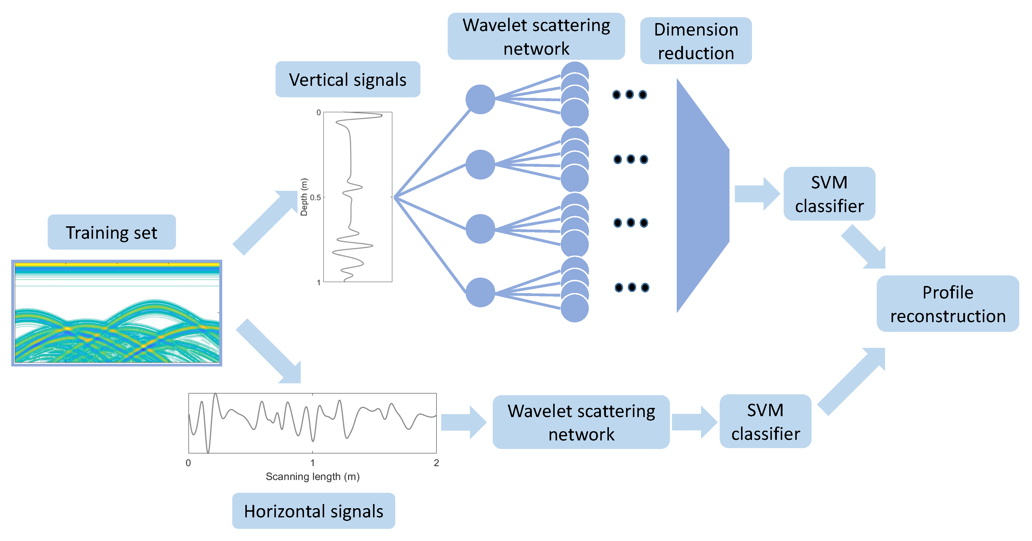
Figure 7.
The machine learning architecture for pipeline identification.
Figure 7.
The machine learning architecture for pipeline identification.
Figure 8.
A brief scheme of profile reconstruction.
Figure 8.
A brief scheme of profile reconstruction.
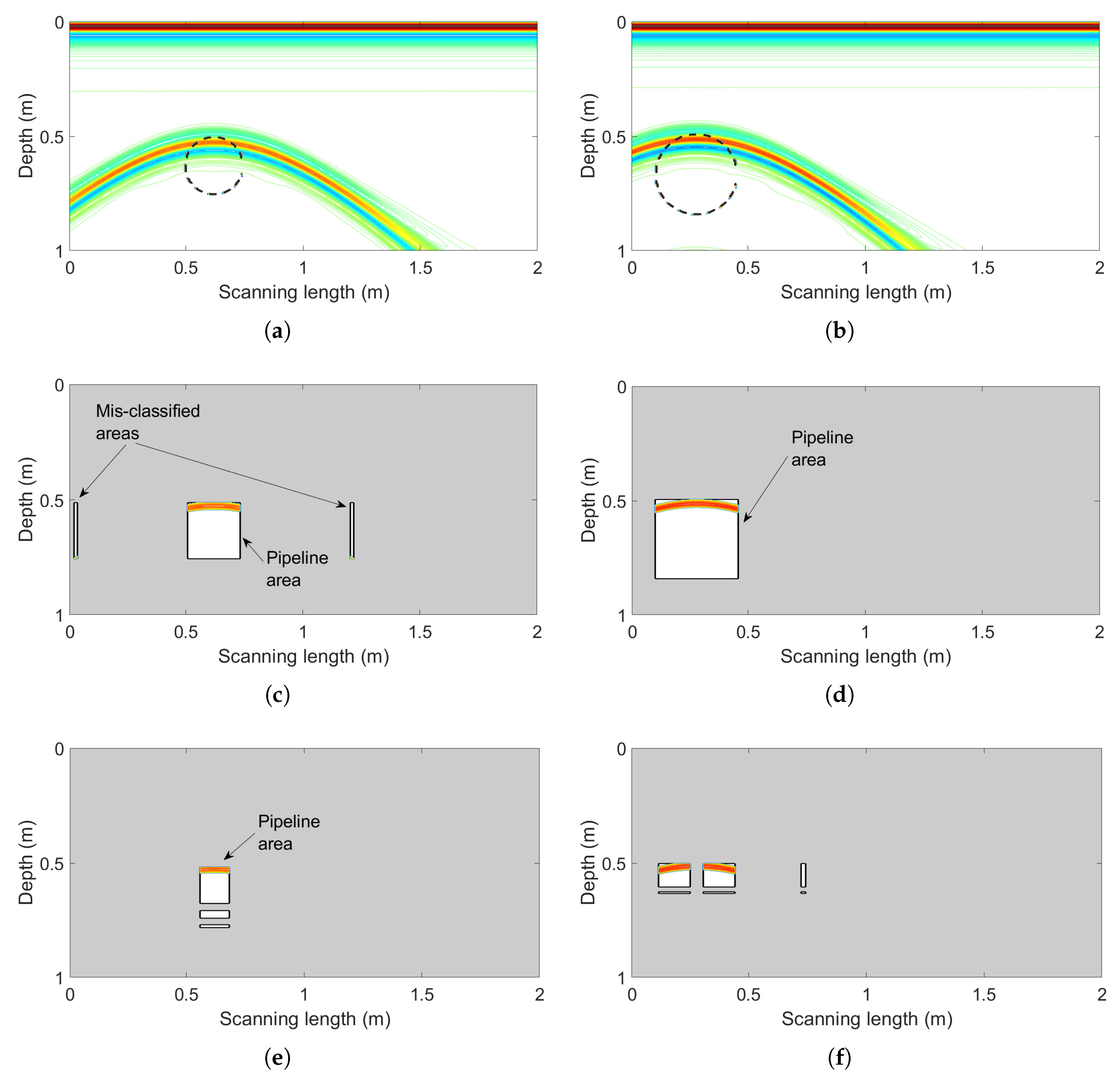
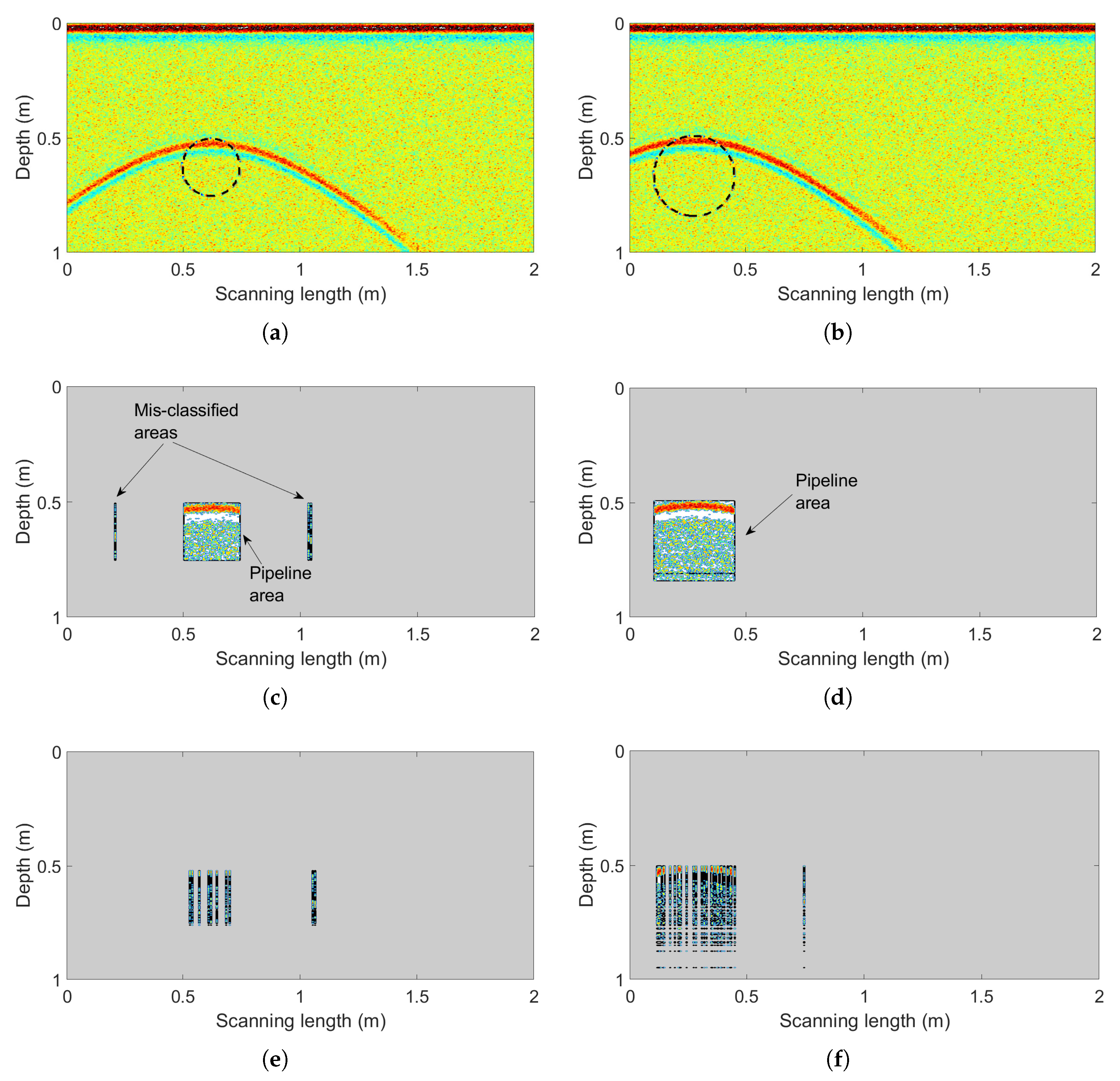
Figure 9.
(a) The example input profile with a single pipeline (central coordinates (0.615 m, 0.63 m), diameter 0.25 m). (b) Another example input profile with a single pipeline (central coordinates (0.275 m, 0.667 m), diameter 0.35 m). (c) The reconstructed profile of panel (a) by the proposed learning framework. (d) The reconstructed profile of panel (b) by the proposed learning framework. (e) The reconstructed profile of panel (a) after the independent SVM for comparison. (f) The reconstructed profile of panel (b) after the independent SVM for comparison.
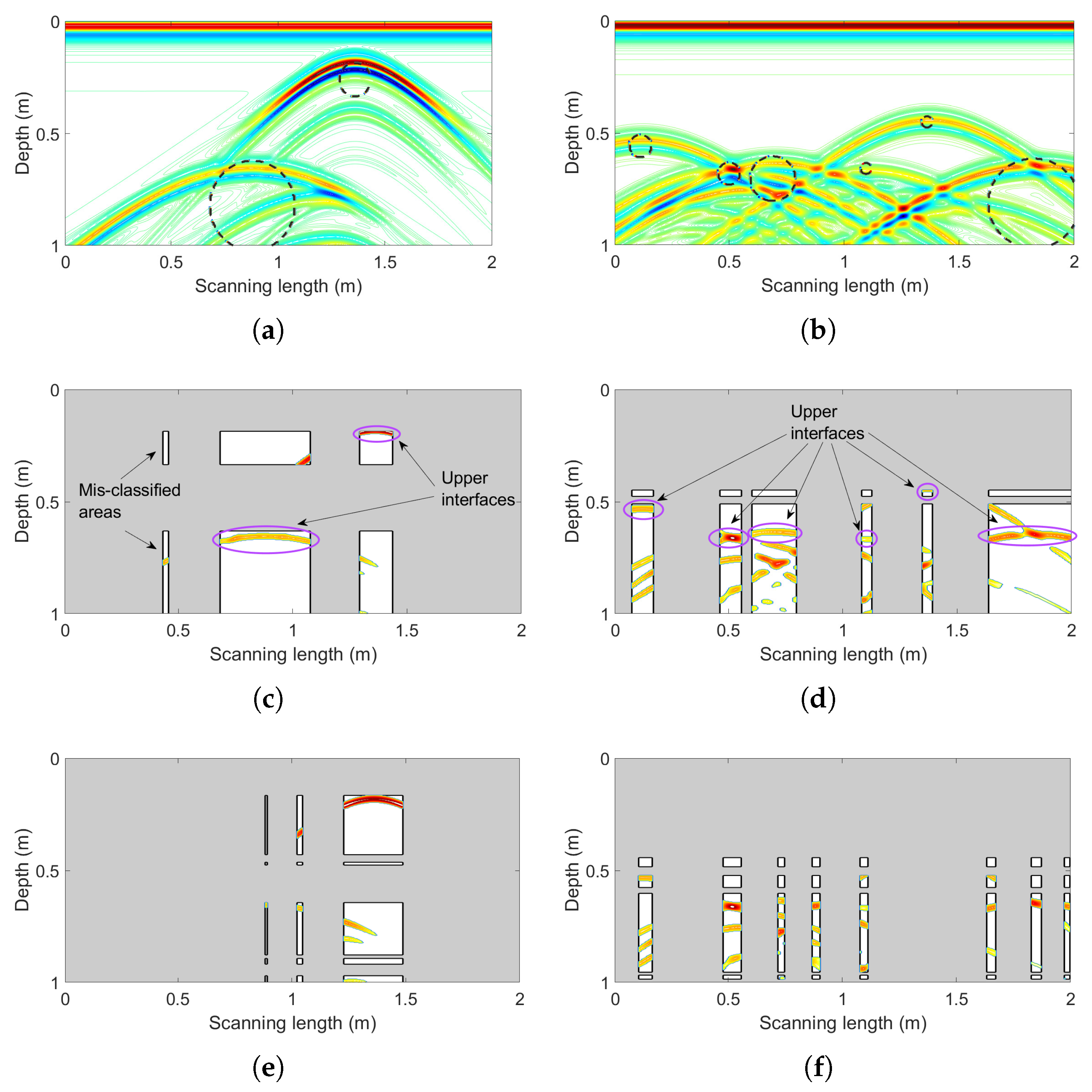
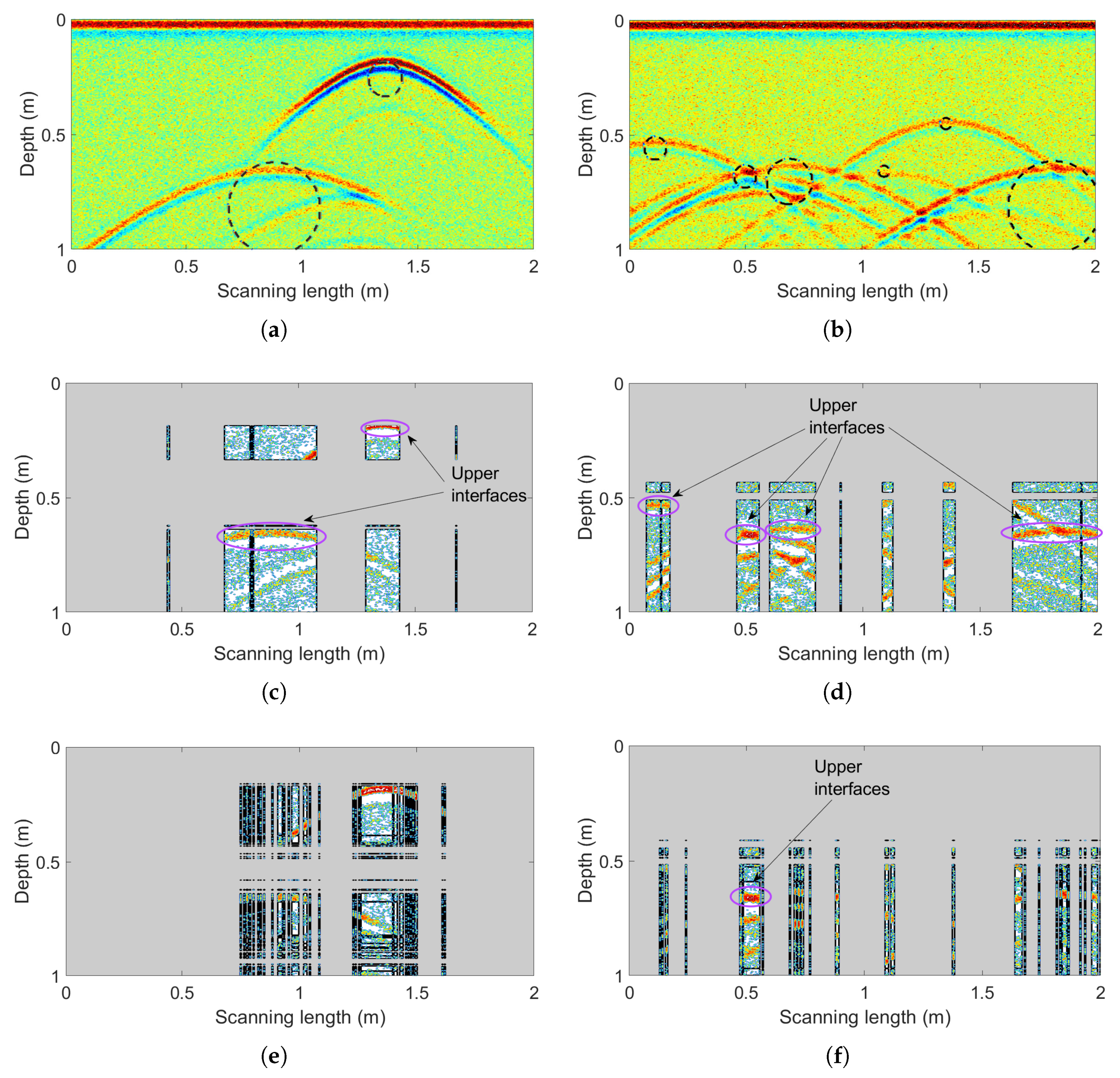
Figure 10.
(a) The example input profile with two pipelines (central coordinates and diameters ((1.355 m, 0.263 m),0.15 m) and ((0.875 m, 0.823 m), 0.4 m)). (b) The example input profile with six pipelines (left five central coordinates and diameters ((0.12 m, 0.56 m), 0.1 m), ((0.505 m, 0.658 m), 0.1 m), ((0.695 m, 0.705 m), 0.2 m), ((1.1 m, 0.66 m), 0.05 m) and ((1.365 m, 0.453 m), 0.05 m), and rightest height and width (0.385 m, 0.37 m)). (c) The reconstructed profile of panel (a) by the proposed learning framework. (d) The reconstructed profile of panel (b) by the proposed learning framework. (e) The reconstructed profile of panel (a) after the independent SVM for comparison. (f) The reconstructed profile of panel (b) after the independent SVM for comparison.
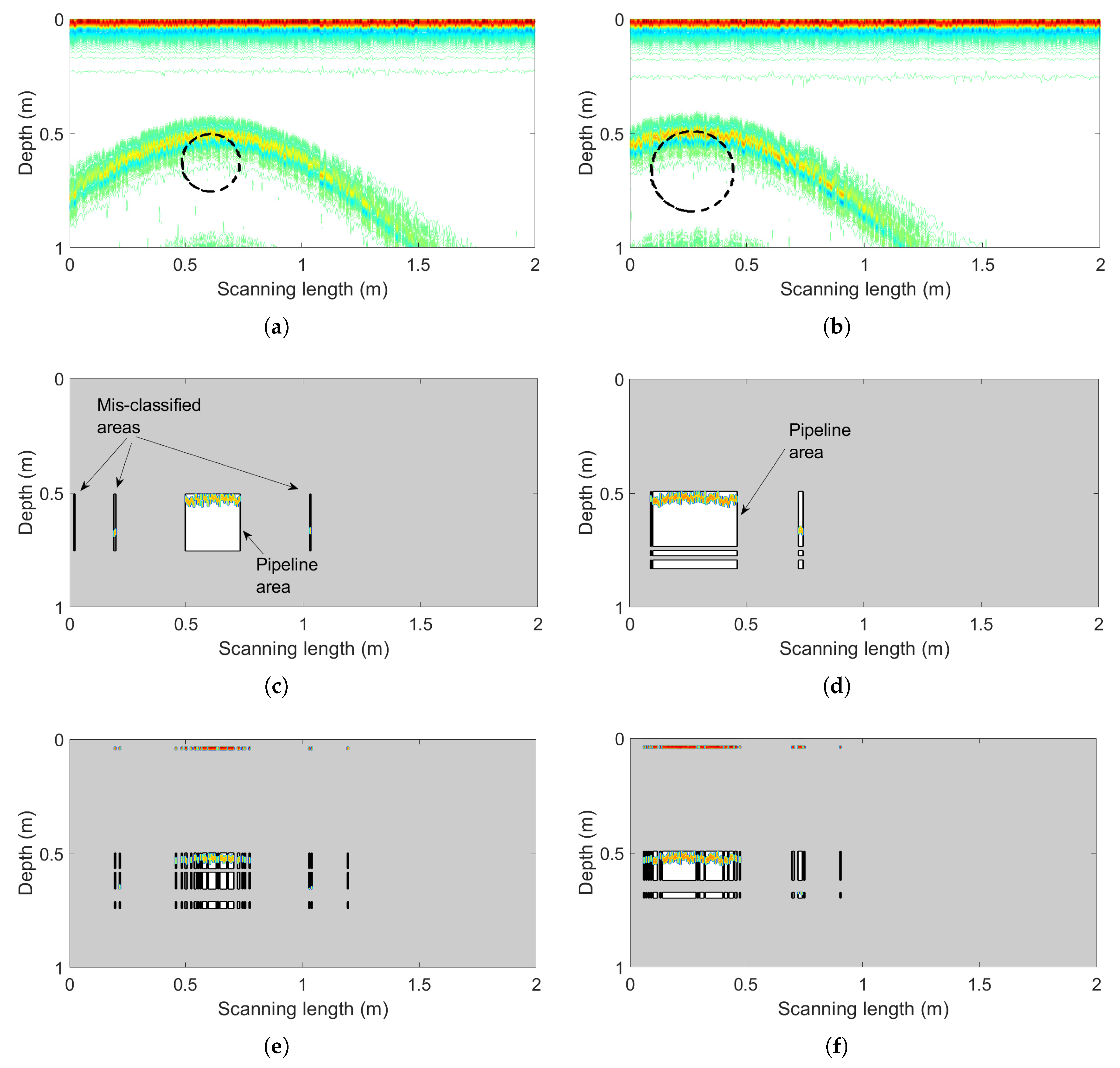
Figure 11.
(
a) The example noisy profile with a single pipeline (seen in
Figure 9a). (
b) Another example noisy profile with a single pipeline (seen in
Figure 9b). (
c) The reconstructed profile of panel (a) by the proposed learning framework. (
d) The reconstructed profile of panel (b) by the proposed learning framework. (
e) The reconstructed profile of panel (a) after the independent SVM for comparison. (
f) The reconstructed profile of panel (b) after the independent SVM for comparison.
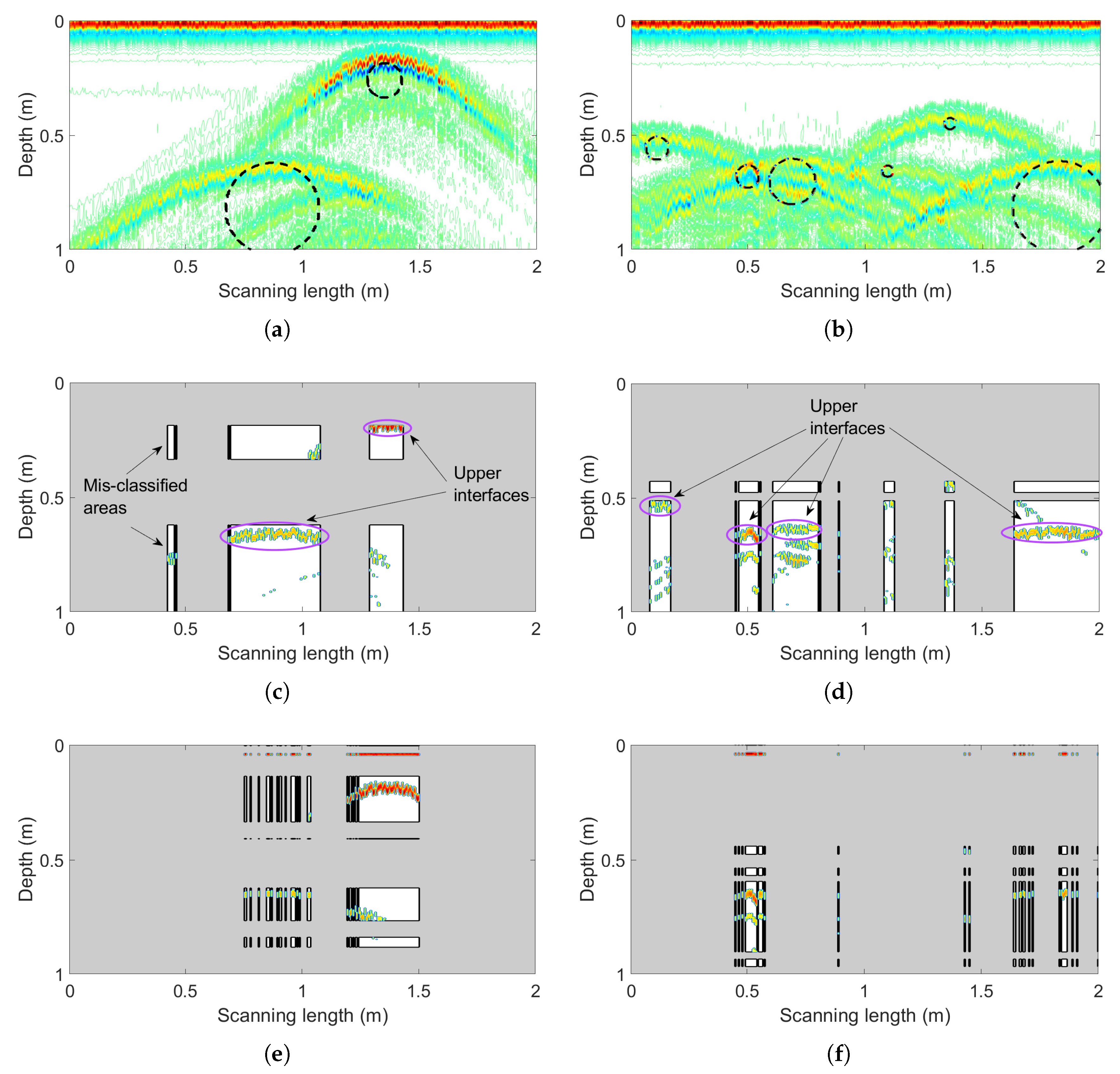
Figure 12.
(a) The example noisy profile with two pipelines (central coordinates and diameters ((1.355 m, 0.263 m), 0.15 m) & ((0.875 m, 0.823 m), 0.4 m)). (b) The example noisy profile with six pipelines (left five central coordinates and diameters ((0.12 m, 0.56 m), 0.1 m), ((0.505 m, 0.658 m), 0.1 m), ((0.695 m, 0.705 m), 0.2 m), ((1.1 m, 0.66 m), 0.05 m) & ((1.365 m, 0.453 m), 0.05 m), and rightest height and width (0.385 m, 0.37 m)). (c) The reconstructed profile of panel (a) by the proposed learning framework. (d) The reconstructed profile of panel (b) by the proposed learning framework. (e) The reconstructed profile of panel (a) after the independent SVM for comparison. (f) The reconstructed profile of panel (b) after the independent SVM for comparison.
Figure 13.
(
a) The example profile with a single pipeline (seen in
Figure 9a) considering surface roughness. (
b) Another example profile with a single pipeline (seen in
Figure 9b) considering surface roughness. (
c) The reconstructed profile of panel (a) by the proposed learning framework. (
d) The reconstructed profile of panel (b) by the proposed learning framework. (
e) The reconstructed profile of panel (a) after the independent SVM for comparison. (
f) The reconstructed profile of panel (b) after the independent SVM for comparison.
Figure 14.
(a) The example profile with two pipelines (central coordinates and diameters ((1.355 m, 0.263 m), 0.15 m) & ((0.875 m, 0.823 m), 0.4 m)) considering surface roughness. (b) The example profile with six pipelines (left five central coordinates and diameters ((0.12 m, 0.56 m), 0.1 m), ((0.505 m, 0.658 m), 0.1 m), ((0.695 m, 0.705 m), 0.2 m), ((1.1 m, 0.66 m), 0.05 m) & ((1.365 m, 0.453 m), 0.05 m), and rightest height and width (0.385 m, 0.37 m)) considering surface roughness. (c) The reconstructed profile of panel (a) by the proposed learning framework. (d) The reconstructed profile of panel (b) by the proposed learning framework. (e) The reconstructed profile of panel (a) after the independent SVM for comparison. (f) The reconstructed profile of panel (b) after the independent SVM for comparison.
Figure 15.
(a) Example input profile with two pipelines (diameter 32 cm). (b) Reconstructed profile of panel (a) by machine learning. (c) Example input profile with 5 × 2 cylinders (diameter 10 cm). (d) Reconstructed profile of panel (c) by machine learning. (e) Example input profile with three pipelines (diameter 50 cm, depth of upper interface 1 m, 1.5 m and 2 m). (f) Reconstructed profile of panel (e) by machine learning.
Table 1.
Accuracy and confusion results of vertical traces with or without wavelet scattering networks in the machine learning model.
Table 1.
Accuracy and confusion results of vertical traces with or without wavelet scattering networks in the machine learning model.
| Models | Training Accuracy | | Validation | |
|---|
| Accuracy | False Positive | False Negative |
|---|
| WaveScat + SVM | 99.73% | 97.94% | 0.91% | 1.15% |
| SVM | 78.59% | 78.44% | 16.87% | 4.69% |
Table 2.
Accuracy and confusion results of horizontal signals with or without wavelet scattering networks in the machine learning model.
Table 2.
Accuracy and confusion results of horizontal signals with or without wavelet scattering networks in the machine learning model.
| Models | Training Accuracy | | Validation | |
|---|
| Accuracy | False Positive | False Negative |
|---|
| WaveScat + SVM | 99.70% | 98.41% | 0.53% | 1.06% |
| SVM | 72.10% | 72.38% | 9.20% | 18.42% |
Table 3.
Accuracy and confusion results of vertical traces (noisy signals) with or without wavelet scattering networks in the machine learning model.
Table 3.
Accuracy and confusion results of vertical traces (noisy signals) with or without wavelet scattering networks in the machine learning model.
| Models | Training Accuracy | | Validation | |
|---|
| Accuracy | False Positive | False Negative |
|---|
| WaveScat + SVM | 99.99% | 94.81% | 2.72% | 2.47% |
| SVM | 84.77% | 76.25% | 14.06% | 9.69% |
Table 4.
Accuracy and confusion results of horizontal signals (noisy signals) with or without wavelet scattering networks in the machine learning model.
Table 4.
Accuracy and confusion results of horizontal signals (noisy signals) with or without wavelet scattering networks in the machine learning model.
| Models | Training Accuracy | | Validation | |
|---|
| Accuracy | False Positive | False Negative |
|---|
| WaveScat + SVM | 99.76% | 94.98% | 2.01% | 3.01% |
| SVM | 82.42% | 67.64% | 12.83% | 19.53% |
Table 5.
Accuracy and confusion results of vertical traces (considering surface roughness) with or without wavelet scattering networks in the machine learning model.
Table 5.
Accuracy and confusion results of vertical traces (considering surface roughness) with or without wavelet scattering networks in the machine learning model.
| Models | Training Accuracy | | Validation | |
|---|
| Accuracy | False Positive | False Negative |
|---|
| WaveScat + SVM | 98.01% | 96.72% | 2.34% | 0.94% |
| SVM | 79.22% | 77.81% | 6.88% | 15.31% |
Table 6.
Accuracy and confusion results of horizontal signals (considering surface roughness) with or without wavelet scattering networks in the machine learning model.
Table 6.
Accuracy and confusion results of horizontal signals (considering surface roughness) with or without wavelet scattering networks in the machine learning model.
| Models | Training Accuracy | | Validation | |
|---|
| Accuracy | False Positive | False Negative |
|---|
| WaveScat + SVM | 98.84% | 97.09% | 1.98% | 0.93% |
| SVM | 78.61% | 76.10% | 19.00% | 4.90% |


