Abstract
Snow makes a great contribution to the hydrological cycle in cold regions. The parameter to characterize available the water from the snow cover is the well-known snow water equivalent (SWE). This paper presents a near-surface-based radar for determining the SWE from the measured complex spectral reflectance of the snowpack. The method is based in a stepped-frequency continuous wave radar (SFCW), implemented in a coherent software defined radio (SDR), in the range from 150 MHz to 6 GHz. An electromagnetic model to solve the electromagnetic reflectance of a snowpack, including the frequency and wetness dependence of the complex relative dielectric permittivity of snow layers, is shown. Using the previous model, an approximated method to calculate the SWE is proposed. The results are presented and compared with those provided by a cosmic-ray neutron SWE gauge over the 2019–2020 winter in the experimental AEMet Formigal-Sarrios test site. This experimental field is located in the Spanish Pyrenees at an elevation of 1800 m a.s.l. The results suggest the viability of the approximate method. Finally, the feasibility of an auxiliary snow height measurement sensor based on a 120 GHz frequency modulated continuous wave (FMCW) radar sensor, is shown.
1. Introduction
1.1. Snow Water Equivalent Importance
Snow makes a large contribution to the water balance, climate, and economy of many regions. The seasonal accumulation of snow acts as a form of natural regulation of great importance in the hydrological cycle. The parameter to characterize the available water from snow cover is the well-known snow water equivalent (SWE). The SWE is the equivalent depth of water available if the snowpack melted into liquid water. This paper presents a near-surface-based technique for determining the SWE from the measured complex spectral reflectance, in the range from 150 MHz to 6 GHz, and an electromagnetic model for the analysis of the reflectance of the snowpack.
As we can see, physical knowledge of the snow cover properties, and, in particular, the availability of field instrumentation to understand them, is crucial. In addition to the most basic hydrological information [1], these measurements provide data to elaborate mathematical models of the climate [2] and the snowpack evolution [3] as well as for avalanche forecasting [4].
1.2. Instrumentation and Techniques
Among the destructive measuring methods of the snowpack, we can find several standard sampling procedures for stratigraphy that are manually performed [5]. Non-destructive methods—mainly, ground-based remote sensing techniques for characterizing the physical properties of snow—have been exhaustively discussed in the literature [5]. Conventional in situ techniques to non-destructively determine the SWE are based on cosmic-ray neutron attenuation (CRN) [6,7], or acoustic signal delays [8], among others. From them, we can directly extract the SWE, but they give no further information about the structure of the snowpack.
The snowpack is a multilayer structure [9], where each layer has its own physical properties, depending on the crystallization form during snowfall and the weather conditions during and after the layer deposition. From a physics point of view, we can consider each layer as a porous body of mixed air with solid and liquid state water. The liquid water content (LWC) is the key parameter to characterize the presence of liquid water [10,11,12].
The only physical entity capable of providing information about the internal structure of a snowpack is an electromagnetic wave in the 100 MHz–6 GHz range [13], where the layers are sufficiently transparent to allow penetration depths in the order of meters. The interaction between electromagnetic waves and the snow is determined by the dielectric permittivity of the latter, which is strongly dependent on its air and water content, and the aggregation state of the water [10,14].
The most promising electromagnetic methods are those based on microwave radar analysis. In fact, over the past 40 years, numerous studies on radar applications for snow cover characterization have been conducted. Impulse waveform radars [15,16] and frequency modulated continuous wave (FMCW) radars [17,18,19,20,21,22,23] have been used to explore snowpack structure.
Until recently, the construction of an FMCW radar, stepped-frequency continuous wave (SFCW) radar, or pulsed radars required an expensive vector network analyzer (VNA) or developing specific electronical equipment [24]. However, a new technology has been developed, the so-called software defined radio (SDR). An SDR system is a radio in which some or all its physical layer functionalities are software defined. A shared feature of all of them is the possibility to generate and detect signals up to 6 GHz, so they are potentially usable for reconfigurable radar system construction [25,26,27,28,29,30].
The recent advances in radar technology, propitiated by automotive radars or SDR, have resulted in low cost and small dimension equipment that will allow portable instrumentation with a high vertical resolution to study properties, such as the depth, stratigraphy, and SWE, of snow cover. The aim of this paper is to show the operation of an SDR-SFCW radar, and the application of an electromagnetic model of the multilayer snowpack to analyze the SWE of snow cover.
This paper is organized as follows. In Section 2, we present the theory of SFCW radar. Section 3 shows the electromagnetic model and the procedure to obtain the SWE. Section 4 focuses on the description of the experimental set-up and the measurement method. Section 5 presents the results and a comparison between the experimental and theoretical results. Finally, in Section 6, we summarize the contributions of the present work.
2. Theory of the SFCW Radar
2.1. Measurement Principle
An SFCW [31,32,33] radar transmits consecutive trains of CW signals of increasing frequency toward a target. The stepped-frequency increment is δf from an initial frequency f0,RF. After receiving the signal at a frequency f0,RF+iδf, with i as an integer, which is delayed in phase as a result of the flight time, a heterodyne process is performed with a local frequency oscillator f0,RF+iδf+fBB, of unity amplitude. The mixing is performed with the harmonic oscillator in-phase with the harmonic function used in transmission (I) and with the harmonic function offset by one quarter cycle (π/2 rads) or in-quadrature (Q) as is shown in Figure 1. After low pass filtering, two harmonic functions at the down converted or intermediate frequency (IF), fBB, are obtained for the ith frequency
where A(R) is the amplitude of the signal received from a target located at an R distance and is proportional to its reflectance, and ϕ represents the phase associated to the time-of-flight. The received IF signals UI(i,t) and UQ(i,t) are multiplied, again, by the signal cos(2πfBBt), and low pass filtered (homodyne process) to obtain the complex amplitude, (i), at each ith frequency of the scan
where c is the speed of light in the vacuum, N the number of frequencies of scan, and I(i) and Q(i) the real and imaginary part of the amplitude (i), respectively. Therefore, if we perform the fast Fourier transform (FFT) with respect to the variable i, we will have an important peak in the dimensionless frequency domain given by
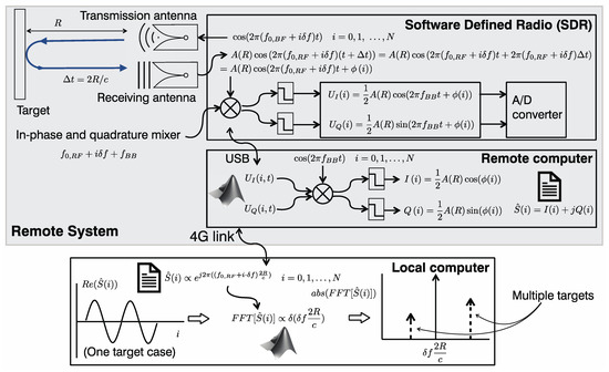
Figure 1.
Structure of a stepped-frequency continuous wave (SFCW) radar system. The gray area is the part of the system that is located in the remote location. Software defined radio (SDR) control is performed in C++ from the remote computer and also computes the spectral reflectance and sends it to the local computer. Both computers develop their algorithms using MATLAB®.
The received spectral reflected signal by targets contains the transit time information or the ‘optical path’ from the target, given by
The FFT resolution, when N frequencies are taken, is given by 1/N. Then, the spatial resolution is given by
which is a well-known relationship in the general radar theory, and where B = Nδf is the bandwidth of the sweep performed by the SFCW radar. The maximum unambiguous range, Ru, can be derived from the periodicity of (3) as
The main disadvantage of an SFCW radar is its long measurement time. In our application, however, the snow cover is a ‘static’ target, and the measurement time is not relevant. The SFCW radar has very narrow instantaneous bandwidth at each frequency due to the narrow low pass filter width at the end of the DC filtering of the and signals, resulting in a high signal-to-noise ratio at the receiver. The bandwidth, B, can be very wide, leading, according to (6), to a fine resolution.
Figure 1 presents the different systems of SFCW radar and its operations. At the remote location, the SDR performs the transmission and reception, obtaining a double IF temporal file ( and ) at each i-frequency of the reflected electromagnetic wave. The remote computer performs the homodyne detection numerically at each frequency. Finally, a file with the complex amplitudes of snowpack reflectance at each frequency is sent to the local computer.
In the case of multiple targets, we obtain a peak associated with the position of each target with the height proportional to its reflectance (Figure 1).
3. Snowpack Electromagnetic Model
Many authors describe wave propagation in snow layered media with recursive relationships of the transmitted and reflected rays, including radiation diffusion and the thermal emission of slabs in the context of radiative transfer models [14]. However, we can simplify the radiative behavior of the snow layers working at long wavelengths compared to the grain size of the deposited snow. In this way, we can minimize the diffusion effects and assume the snow layers as homogenous and isotropic media with wavelength dependent and complex dielectric permittivities to take into account the attenuation of radiation. We used the 2 × 2 matrix method that is typically employed in planar multilayer optical structures and extensively described in the literature [34,35].
3.1. Matricial Multilayer Snowpack Electromagnetic Model
The matrix formulation is an extremely useful form of the steady-state solution of Maxwell’s equations subjected to the boundary conditions imposed at the interfaces of a multilayer stack with n + 1 media where the upper and lower media are semi-infinite, and the number of layers is n − 1 (Figure 2). Maxwell’s equations reduce to independent sets of equations for the transverse-electric (TE) and transverse-magnetic (TM) polarizations. The TE polarization has the electric-field vector E perpendicular to the plane of incidence, whereas the magnetic-field vector, B, is transverse in the TM case.
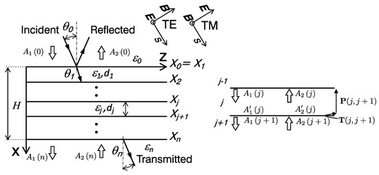
Figure 2.
An n + 1 media structure (n − 1 layers) of snowpack of height H. The relative dielectric permittivities are, in general, complex magnitudes. The upper and lower media are semi-infinite.
According to Maxwell’s equations, the general expression for the TM polarization of the x component of electric field in layer j can be written as
where A1 represents the amplitude of a planar wave propagating in the positive x, and z, direction and A2 represents a plane wave propagating in the negative x direction and positive z direction, k is the wavenumber in vacuum and nj is the refractive index of the jth slab related to the relative dielectric permittivity.
By replacing solution (8) in the Maxwell’s equations, we obtain the general expression of the electric and magnetic fields for TM solutions in jth medium
The relationship between the coefficients A’1(j), A’2(j), A1(j + 1), and A2(j + 1) corresponding to the amplitudes on one side and the other of the interface (j) − (j + 1), (Figure 2 right), is given by the continuity of the tangential components of the fields. We can summarize this relation in a matrix form
The coefficients A’1(j) and A’2(j) on the interface (j) − (j + 1) are related to the coefficients A1(j) and A2(j) of the same layer but at the interface (j − 1) − (j) by the propagation matrix P(j)
The recursive application of the boundary conditions at the interfaces and the propagation for E and B through the layers, leads to a relationship between 0 and n amplitudes given by
Similarly, we can obtain the transmission matrix for TE polarization, but, in our particular case, as the angle of incidence is null, the two polarizations are equivalent. In a general case, the transmission matrix from the j + 1 to j layer for TE polarization is
3.2. Reflectance Calculation for the Snowpack Multilayer
According to the formulation outlined before, the complex reflectance, Γ, of the snowpack, and assuming the condition that there is no upward propagating wave in the medium n, i.e., A2(n) = 0, is given, in the TE or TM case, by
therefore, to calculate the reflectance of the snow cover, we calculate only the M21 and M11 elements of the M matrix, according to expression 18. This is the amplitude reflectance of a plane wave (TE or TM) incident from medium 0 with an angle and reflected with the same angle.
3.3. Spectral and Spatial Reflectance of Snowpack
According the theory of SFCW radar, in the scan process we obtain the reflectance in N frequencies, i.e.,
The relation between spectral and temporal (spatial) reflectance can be derived by means of FFT.
or in function of distance, R,
with represents the “spatial reflectance” that comes from different distances.
3.4. Complex Dielectric Constant of Dry and Wet Snow
To simulate the reflectance of a multilayer structure, a complex relative dielectric permittivity model for dry and wet snow in the 150 MHz to 6 GHz band is needed. We have used the empirical formula from Tiuri [10]. In the literature, however, there are other models such as the one proposed by Wiesmann [14], but the permittivities calculated by the two models are practically the same.
Figure 3 shows the frequency behavior of dielectric permittivity for dry snow and wet snow with a liquid water content (LWC) of 2% and a relative density of 0.2.
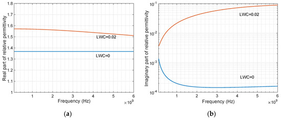
Figure 3.
Relative dielectric permittivity of snow from 100 MHz to 6 GHz for dry snow and wet snow with a liquid water content (LWC) of 2% and a relative density of 0.2: (a) Real part of the relative permittivity. (b) Imaginary part of the relative permittivity.
We can see the remarkable effect of the presence of water in liquid form both on the real part and, particularly, on the imaginary part. The presence of water in liquid form will have an important impact in the penetration depth of radiation into the snowpack.
3.5. Simulations of Snowpack Reflectance
To show the behavior of the reflected spatial signals of the SFCW radar, we analyzed several cases calculated with the matrix method. A sweep from 150 MHz to 6 GHz was used in 15 MHz steps (N = 390).
A 1.5 × 1.5 m piece of sheet metal was incorporated into the soil in the experimental structure to improve the reflectance of the snowpack–soil interface. The relative permittivity considered for this layer (nth) was j50. Matrix calculations to simulate the spectral and spatial reflectances, Γ(i) an Γs(i) respectively were graphically implemented (Figure 4) in interactive software. Experimentally measured traces can be imported into the application to compare with the theoretical traces calculated with the matrix method.
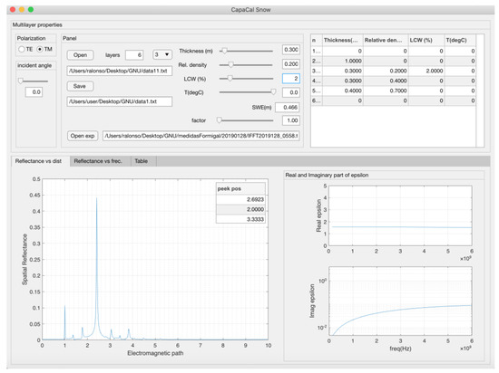
Figure 4.
Software developed to calculate the time signal of radar for a snowpack, including the density, wetness, and frequency of all layers. (Adapted with permission from ref. [30]. Copyright 2020 IEEE).
Figure 5a presents the reflectance of the signal produced by the aluminum sheet (orange line) located 2 m away from the origin. This is a reference reflectance in the next graphs. On the same graph, we overlap the radar reflectances in the cases of one-meter snow layer with relative density 0.3 and one-meter snow layer with relative density 0.6. A first reflection on the upper face associated with the air–snow interface can be observed. The position of this first reflection relative to that of metal without snow cover (orange), allows us to know the height of the snow cover, H.
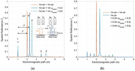
Figure 5.
SFCW simulated spatial reflectances with the matrix method: (a) Signals for a 1 m of air and 1 m of snow layer with 0 (air), 0.3, and 0.6 relative densities. The orange line represents the reflectance of metal without a snow cover. (b) Air + three-layer structure with thicknesses [1,0.3,0.3,0.4] and relative densities [0,0.2,0.4,0.6]. We use an array format to describe the thicknesses and densities of layers.
We also observed how the reflection of the metal layer moves to the right as a result of the flight time inside the snow cover. In the case of a relative density of 0.6, there was a greater displacement. Finally, there are symmetrical peaks (3 in Figure 5a) that are the second reflections in the snow cover as is indicated in the draw included in Figure 5a. More reflections are observed with difficulty; however, it is necessary to note that even the case of dry snow, there is an attenuation (see Figure 3b) that reduces the magnitude of the successive reflections.
Figure 5b shows the superposition of the metal plate signal with a slightly more complex structure than the previous one. Specifically, there are three layers of thicknesses of 0.3, 0.3, and 0.4 m with relative densities of 0.2, 0.4, and 0.6, respectively. We can see how, again the first reflection, positioned at the height of the snow cover. There are some reflections between the different interfaces of the structure. These internal reflections are very small in magnitude compared to the reflectance of the air–snow and snow–metal interfaces.
In Figure 6, we can see the effect of the wetness on the structure of Figure 5b. Increasing the wetness of the layers results in a higher reflectance at the air–snow interface. This effect is due to an increase in the real part of the permittivity as a result of the presence of liquid water. Likewise, for this same reason, there is a slight increase in the optical path as is evident in the rightward displacement of reflection on the sheet metal as the content in liquid water increases. Finally, the effect of the imaginary part is seen in the drastic reduction of reflectance in the sheet metal and all other secondary peaks. Note that we reduced the vertical scale to see them.
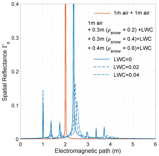
Figure 6.
SFCW radar simulated spatial reflectances with the matrix method. Effect of wetness (LWC) in the reflectance (blue lines). Thicknesses (m) = [1,0.3,0.3,0.4]. Relative densities of the structure = [0,0.2,0.4,0.6], LWC = 0 (solid line), 0.02 (dashed line), and 0.04 (dot-dashed line).
3.6. Estimation Procedure of SWE
Figure 7 shows the effect of the layer density on the position on the reflectance of the snow–metal interface of 1-m-thick snow of relative densities of 0, 0.2, 0.4, 0.6, and 0.8. We can observe a linear displacement of the peaks, proportional to the relative density of the layer (ρ).
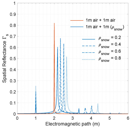
Figure 7.
SFCW radar simulated spatial reflection of a 1 m snowpack with the relative densities 0, 0.2, 0.4, 0.6, and 0.8.
In view of this effect, and according to the definition of the snow water equivalent for a multilayer (n + 1 media) particularized to one-layer snowpack
we can conclude that there is a linear relationship between the SWE and the position of reflection on the sheet metal when it is covered by a layer of dry snow. This relationship, a priori, is not obvious. Indeed, the position of the snow–metal peak is determined by the optical or electromagnetic path, which depends linearly on the refractive index of the layer, while the SWE is density related. However, we have just seen the proportionality between them. We can check this fact in the case of dry snow. In fact, using the empirical expression proposed in [10,14], we can observe that the real part of the square root of the relative dielectric permittivity is approximately linear with the snow density as shown in Figure 8—i.e., the real part of the refraction index of dry snow is proportional to the density [17]. Then, we can assume a relationship between the real part of the refractive index, n’, and the relative density given by
where Re denote the real part of a complex number. Factor a in the above equation is obtained from a linear fit of Figure 8 (a = 0.844).
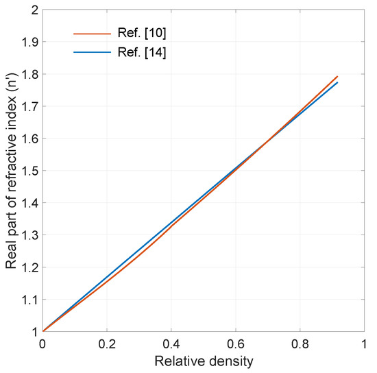
Figure 8.
Real part of refractive index vs. the snow density at a frequency of 1 GHz and 0% LWC. Results using [10,14] are represented by blue and orange lines, respectively. The linear fit gives n’(ρrelative) = 1 + 0.8439ρrelative.
Then, the ‘flight time’ or ‘optical/electromagnetic path’, D, into the snow structure, which is the distance between the air–snow peak and the snow–metal one, can be written as
where n’i is the real part of refractive index of the ith slab, of thickness di, and H is the snow depth. Then, we have confirmed the relationship between the optical path and the SWE, which justifies those discussed in relation to Figure 7. The displacement position (see Figure 5a) of the snow–metal sheet reflection peak with respect to the position of the sheet in the air, ΔD, is given by
Figure 9 shows the comparison between the SWE vs. ΔD calculated with the previous expression (solid line) and the one provided by the displacement of the metal reflection by means of the matrix model (circles), for a layer 1 m thick and densities from 0.2 to 0.8 (SWE from 0.2 to 0.8 m). Accordingly, we can conclude that the SWE of a snowpack is intrinsically related to its electromagnetic thickness. The measurement of the SWE by this approximate procedure is independent of the measurement of the height of the snow cover—we should only need to know the displacement of the snow–metal reflection relative to the position without snow cover, to obtain the SWE.
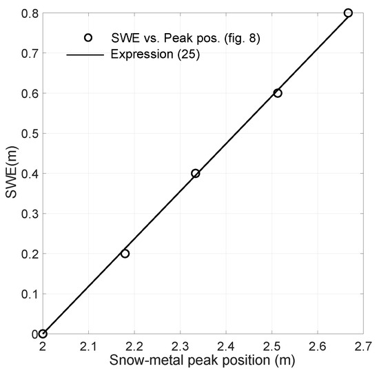
Figure 9.
Comparison between the SWE and the displacement of the metal reflectance for the structure of Figure 7 by matrix simulation (circles) and the analytical expression 25 (solid line) assuming linearity of the real part of refractive index vs. the density.
4. Materials and Methods
4.1. Test Site Description
The experimental validation of our SFCW radar was carried out at the Formigal–Sarrios test site located in the Spanish Pyrenees (42°45′40.6″N 0°23′31.8″W) at an elevation of 1800 m a.s.l. (Figure 10). The site was the Spanish location established by the Spanish State Meteorological Agency (Agencia Estatal de Meteorología (AEMet)) in the World Meteorological Organization Solid Precipitation Intercomparison Experiment (WMO-SPICE) [36]. Currently, the site is equipped with sensors to continuously record the meteorological and snow properties. This installation, managed by the territorial delegation of AEMet in Aragon, is an exceptional laboratory for cryosphere studies since it has underground electrical infrastructure, broadband communications, real-time video feeds of the different experiments, a small warehouse with work tools as well as has easy access in the winter, as it is located inside the ski resort Aramón-Formigal. It is a closed area with restricted access and is maintained by the ski resort staff.
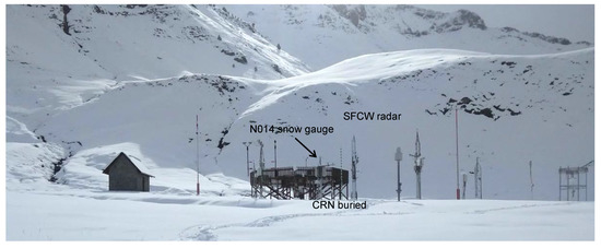
Figure 10.
The AEMet Formigal–Sarrios test site located in the Spanish Pyrenees (42°45′40.6″ N 0°23′31.8″ W) at an elevation of 1800 m a.s.l. The cosmic ray neutron gauge (CRN) N014 from the Automatic Hydrologic Information System of the Ebro River Basin (SAIH-CHE) is buried by the snow. The SFCW radar is located near the CRN.
It is located in a safe area where a stable snowpack is available from mid-November to May, reaching up to 2 m of snow thickness. Due to its flatness and low exposure to the winds, it has a very homogeneous snow cover through the area of experimentation.
We compared our results with the SWE cosmic ray neutron attenuation gauge (CRN) #N014 [37] from Automatic Hydrologic Information System of the Ebro River Basin (Sistema Automático de Información Hidrológica de la Confederación Hidrográfica del Ebro (SAIH-CHE)), located 10 m away from the SFCW radar measurement area (Figure 11b).
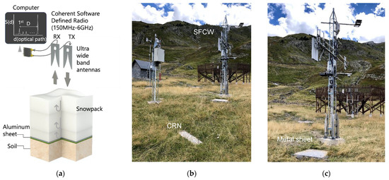
Figure 11.
(a) Diagram of the SFCW radar measurement process. (b) The SAIH-CHE N014 CRN gauge in soil. (c) Prototype of the SFCW radar and metal sheet.
4.2. Field Measurement Radar Setup
The SFCW radar was implemented using a SDR platform. Currently, SDR is one of the emerging areas of research in low cost and accurate radars. The radio frequency oscillator, the receiver ultrawide band amplifier, the demodulator, and the analog-to-digital converters were programmed in low level software in a high-performance SDR USRP X300 with a daughter coherent board UBX 10–6000 MHz from Ettus Research. The final system was a coherent and full-duplex wideband transceiver that covered frequencies from 10 to 6 GHz (see Figure 11a). SDR control was performed in C++ from the remote computer located in the experimental field, which also processes the IF signals at each frequency of scan to, finally, obtain the complex amplitude of the reflected signal vs. frequency.
The data are requested by a local computer from this remote system via a 4G link. The FFT of the signals and the visualization is performed on the local computer. Both computers develop their algorithms using MATLAB®. A detailed picture of the processes being carried out is shown in Figure 1 in Section 2.1. Finally, the system used aluminum Vivaldi transmitter and receiver antennas (UWB3 from RFSpace) placed next to each other and protected with two radomes. Both antennas also included a heater system (Figure 12a) to avoid undesirable freezing problems. It has been verified that the radiant parameters (S11) of the antennas were not modified, from 150 MHz to 6 GHz, by incorporating the heaters.
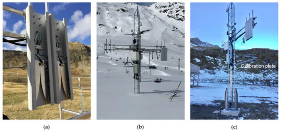
Figure 12.
(a) Detail of the emission and reception antennas. At the bottom, we can see the heating resistors. (b) Overview of the complete system showing the flatness of snowpack in the work area. (c) Virtual “0” calibration plate (CP) placed at 254 cm of the metal sheet.
Finally, an aluminum sheet of 1.5 × 1.5 m (see Figure 11c) was placed on the ground in an orthogonal direction to the antenna’s axis and was the n-medium of the stack with an intrinsically imaginary behavior of relative permittivity. This sheet was buried underneath the snowpack during the entire snow-covered period. Table 1 summarizes the main parameters of the radar.

Table 1.
SFCW radar specifications.
A small weather station, CR300 unit, and a temperature gauge from Campbell Scientific, was included in the system to systematically record the temperatures and activate antenna heaters when the outside temperature dropped below 4 °C.
For calibration purposes, a temporal metallic calibration plate (CP) was placed at a position between the soil and antennas and represents a virtual position that we call ‘0′ and a reference signal to obtain the spatial reflectance of snow cover. In our system, this was located 254 cm from the metal platform on the soil. This CP was also used to optimize the receiver gain in each frequency of the chirp. The measured file generated, represents a complex amplitude array reference for the succeeding measurements as we will see later. We have selected this position for the definition of the origin to be able to perform calibrations also in the winter period if necessary. In addition, the choice of this origin simplifies the interpretation of spatial reflectance signals by being all of the same sign.
4.3. Measurement Process
The remote computer, controlled by the local computer, runs a C++ program in which the SDR transmitted and received 390 frequencies between 150 MHz and 6 GHz. The duration of this sweep was approximately 80 s. The IF used (fBB) was 31.25 kHz and was sampled at a rate of 3.125 MHz. The received signal at each frequency UI(i,t) and UQ(i,t), was multiplied numerically by the signal at fBB frequency, and low pass filtered to obtain the magnitude and phase of the amplitude received at each frequency. This file, , was sent via the 4G link to the local computer.
The measured spectral amplitude is divided by that measured with the calibration plate, . The spectral reflectance is, then, calculated as
Subsequently, the FFT of was performed to obtain the spatial reflectance, , the file with time and date identification was archived, and a real-time graphical representation was made. The definition of reflectance given in expression 18 requires the use of plane waves according to the theoretical model. In the experimental situation, this is not possible due to the proximity of the antennas to the snow cover, so the experimental reflectance given by (26) is not exactly that given in (18), but in normal incidence will be proportional. For this reason, we have not used a different symbol for both cases. In the graphs, , vs. electromagnetic path the most important information is the spatial position of the peaks and their relative magnitudes.
On 25 January 2019, before the first important snowfall of 2019, the SFCW radar was operative. A previous series of measurements of the distance of metal sheet on the soil (2.54 m) were made with the radar to later obtain the height of the snow cover.
In Figure 13a, we can see the comparison between the measurement of the position of the sheet without snow cover, and the reflectance with a thickness of 61 cm of snow. The reflectance position on the snow–metal interface moved to the right as a result of the increased flight time due to the refractive index of the snow cover. Reflection on the air–snow interface was also observed symmetrically, from which it is possible to deduce the geometric height of the snow cover. According to expression 25, we can, thus, obtain the SWE. The position of the first peak associated with the air–snow interface was 1.923 m, and considering that the reference position of the sheet metal was 2.538 m, we obtain a depth of 61 cm. On the other hand, the displacement of the snow–metal interface was 2.667 m − 2.538 m = 0.129 m. Expression 25 allows us to obtain the SWE as 0.129 × 1.185 = 0.153 m.
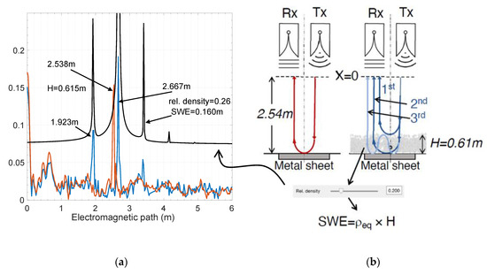
Figure 13.
(a) Comparison of the experimental spatial reflectance obtained for a snow layer 61 cm deep and the one simulated by the matrix model. (b) Outline of the model adjustment procedure with the experimental curve using the density slider of the visual program.
The reflectance simulation by means of the matrix model was superimposed. To fit the theoretical reflectance to the experimental one, it was necessary to adjust the density of the layer of height 0.61 m, to 0.26, and then the SWE using expression 21 is 0.26 × 0.61 = 0.158 m, which is similar to the previous result and confirms the validity of the proposed model.
4.4. Milimeter Wave Radar Depth Sensor
In January 2020, to reinforce the measure of the snow depth, we incorporated a millimeter wave radar sensor (mmWave). The rapid evolution of radars has generated, in the last years, the so-called mmWave sensors, characterized by their small dimensions, low cost, and high processing performances, which were unthinkable a few years ago. In many of them, the transmitter, the receiver, the antennas, the low noise amplifier, the mixer, and the pre-processing are included in a single chip.
Currently, we use the sensor MMIC TRX_120_001 of Silicon Radar [38]. This integrated circuit operates in the band for industrial, scientific, and medical (ISM) purposes of 120 GHz (λ = 2.5 mm). These components, halfway between photonics and microwaves, are practically handled as photonic devices and components based on plastic materials—such as lenses, guides, etc.—are typically used in this technology. Due to its rapid development, the application fields are yet to be determined. An example of this fact is the application proposed.
Snow height measurement is typically performed using ultrasonic sensors by measuring the flight times of a pulse emitted by the transducer and reflected by the snow surface. However, the low acoustic reflectance of the first layer, in particular, in the case of fresh snow with a high air content, is very small, generating noisy signals. In addition, achieving good accuracy requires compensation of the propagation speed with the temperature, which greatly complicates achieving high accuracy.
The use of an FMCW radar at 120 GHz and a bandwidth of 6 GHz, based on Silicon Radar MMIC TRX_120_001 IC, at a normal incidence toward the snow allowed us to obtain sufficient accuracy to verify the height measurement of the SFCW radar. As we have already seen in the examples calculated with the matrix method, the reflectance of the first snow layer in the 1–6 GHz band was very small. This is a consequence of the slight change in the refractive index between the air and the first surface of the snow cover, especially for low-density, fresh snow. However, at frequencies of 120 GHz, there is a low penetration of waves in the snowpack, as the relative permittivity models foresee; nevertheless, there is a strong surface reflectance dominated by diffusion rather than optical reflection by the refractive index change. This effect is a consequence of the use of wavelengths comparable to the surface grain of the snowpack. In Figure 14, we can see the implementation of this auxiliary system.
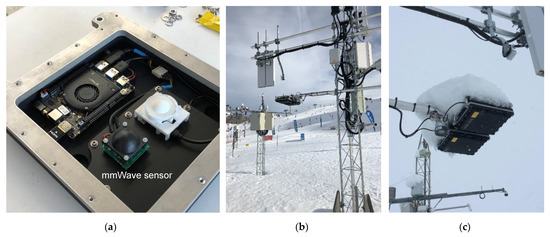
Figure 14.
(a) 120 GHz FMCW mmWave radar sensor with a collimation lens manufactured in plastic. (b) Position of the height sensor near the SFCW radar antennas and outside its field of view. (c) Bottom view of the system.
5. Results
In this section, we describe the main results obtained during the winter period from 1 November 2019 to the 1 May 2020.
Figure 15 shows two examples of range profiles made on the 1 and 20 of March 2020. The orange curve represents the reflectance of the metal sheet registered before the winter period. This is the reference reflectance for the measurement of the geometric height, H, as well as the SWE of the snowpack. Figure 15a clearly shows the profile of a signal as predicted by the matrix model of the snowpack: an important reflectance of the snow–metal interface and a smaller one corresponding to the air–snow interface, as well as the secondary reflection close to 3.5 m of the electromagnetic path. This measure corresponds to a period with low night temperatures, which implies that at the LWC of the snow was small, which justifies the appearance of the secondary reflection.
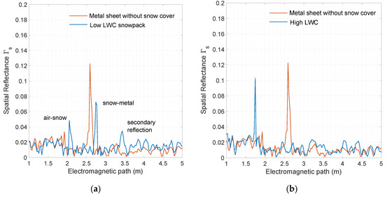
Figure 15.
Spatial reflectances of two measurements compared with the metal sheet without snow cover case (orange): (a) 1 March 2020, 1:18 AM; (b) 20 March 2020, 3:24 AM.
We observe a lower height of the reflectance of first peak compared to the snow–metal one, as predicted by the matrix model (see Figure 5a). Figure 15b shows the measure made in the early morning of the 20 March, after a period of high temperatures even at night. In this case, we see a more intense reflectance peak than in the previous case associated with air–snow reflection, the disappearance of the snow–metal interface reflection, and, of course, the secondary reflection. This situation corresponds to the one shown in Figure 6a, but with a LWC greater than 4%. In this situation, it is not possible to measure the SWE; however, it is possible to measure the geometric height.
In these figures and the following ones, it is not possible to see the transitions between layers as seen in Figure 5b of the model. These internal reflections are very small and, to see them, we would need to improve the signal-to-noise ratio of the radar. However, it is also possible that the strong transformations produced in the snowpack in the Pyrenees, with wide thermal fluctuations and strong solar irradiations can produce smoothing of these interfaces and transform the multilayer structure to a single-layer structure, from an electromagnetic point of view, in a short time.
In Figure 16a, we depict the measured range profile from 8 March, after a significant snowfall, and an elevation of temperatures with an increase of the LWC, also produced a very wet surface layer magnifying the air–snow reflectance even more (see Figure 6a). However, in Figure 16b, just a few hours later, in the early morning of 9 March, we observed the refreezing of the structure, with a decrease in the air–snow reflectance, due to the reduction of the LWC, and the appearance of the displaced snow–metal reflection, 2.92 m − 2.54 m with respect to the reference reflectance, indicating about 0.44 m of SWE according to expression 25.
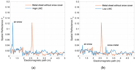
Figure 16.
Spatial reflectances of two measurements compared with the metal sheet without snow cover case (orange): (a) 8 March 2020, 4:46 PM; (b) 9 March 2020, 1:45 AM.
In Figure 17, we can compare the profiles of reflections of a cold period (20 January) that was somewhat sunny, where dry and little-transformed snow predominates, with a warmer period (1 April) with a high content of liquid water. In the first case (Figure 17a), the lower air–snow reflection was lower than that of the snow–metal, which moved to the right. In Figure 17b, we only see a reflection on the upper face of the snow cover.
Figure 17.
Spatial reflectance of two measurements compared with the metal sheet without snow cover case (orange): (a) 20 January 2020, 7:02 AM; (b) 1 April 2020, 3:53 PM.
Figure 18 shows a summary of the conditions under which the experiment was developed. The upper graph shows the temperatures recorded throughout the measurement period. This information is important since the snowpack is exposed to periods with temperatures higher than 0 °C, even at night.
Figure 18.
Evolution of certain magnitudes of interest from 1 November 2019 to 1 May 2020. In the figure above: Temperatures recorded in the position of the radar SFCW. Central figure: Graphic chart of the evolution of reflectance profiles over time. Figure below: Height comparison between the millimeter wave radar sensor and the CHE ultrasonic probe (N014) and snow water equivalent (SWE) measured by the SFCW radar and the CHE CRN N014.
The central chart represents an image of the space-time profiles recorded over the measurement period. In this image, it is possible to appreciate the time intervals in which the reflections of the air–snow interface or the snow–metal interface predominate.
In the lower image, the measured depths of snow cover and the SWE are represented. Depths measured with an ultrasonic sensor located in the position of the CRN probe, are compared with the measurements carried out with the mmWave sensor described in Section 4.4. Finally, the comparison between the SWE measured by the CRN probe and that obtained from the spatial profiles by measuring the displacement of snow–metal reflection in accordance with the expression 25 is shown.
We observed in the central image that, toward the end of the winter period, the reflection on the metal sheet was weaker due to the greater LWC compared with in the early part of winter. However, it was possible to find areas where the reflection was recovered, and it was, therefore, still possible to obtain the SWE. In the central chart, it is not possible to see them; however, a detailed analysis of the profiles allows one to locate those reflections. We have represented them by points in the graph below in Figure 18. This effect focuses on the periods located in the second half of April and the first fortnight of May, in which only some useful points can be recovered.
In the center chart, a reference line was plotted at the 2.54 m position, and the magnitudes of interest provided by this chart are indicated. First is the geometric height, H, which is the distance between the reference line and the upper reflection (air–snow). The maximum height reached in early March is also noted. Secondly is the electromagnetic path, D. Finally, the displacement of the reflection of the snow–metal interface, ΔD, represents the variation of the electromagnetic path from that in the air. This distance directly contains information about the SWE of the snowpack, regardless of the height of it.
The lower graph depicts the depth of the snow cover measured by the ultrasonic sensor located in the position of the CHE tower N014 (blue) and the one measured by the mmWave sensor (black), located about 10 m from the previous one, and which became operational in January 2020. We can see differences of about 20 cm that were proven to correspond to the irregularity of the terrain.
However, several manual depth measurements were also made in the SFCW measurement area, and the correct height measurement was checked. Manual depth measurements are represented with triangles. The first measurement, with a portable depth rod, took place on 8 December 2019, when the mmWave sensor was not yet installed; however, the information can be checked with that provided by the SFCW, being coincident with the manual testing. This comparison is possible for other points, being correct as well.
The two lower curves represent the SWE provided by the CRN gauge (blue) and the SWE obtained by the SFCW radar (black), which was slightly lower than the previous one. Again, the terrain irregularities between the two measurement points would justify this difference. The presence of the metal sheet can modify the drainage properties of the natural soil, retaining more liquid water. This effect would explain that, in some periods, there was the same accumulated water with less snow height. This situation must be corrected in the future, replacing the opaque sheet metal with a semi-buried wired metallic mesh that modifies the properties of the natural soil as little as possible. As the minimum wavelength in the vacuum used by the radar SFCW is 5 cm, a wired mesh with centimeter-order openings would remain effective as a reflector and would not significantly modify the natural soil drainage.
In the second half of April, there was a mismatch between the height and SWE measurements for both the radar SFCW and SAIH-CHE’s N014 system. This is because the height sensors are closer to the towers than the measurement position of the SWE. This fact is not significant for thicknesses greater than 20 cm, but for lower thicknesses, the tower carrying all the elements acts as a hot spot making the snow layer disappear more quickly in its vicinity than in the measurement area of the SWE.
On the black curve, there is a period between 4 and 17 December in which the SFCW system was not operational.
6. Conclusions
This work shows the validation of the proposed SFCW radar technique, based in a RDS system, and an electromagnetic model of snowpack, to obtain its SWE and depth, in real time, for hydrological purposes. The RDS technology has been shown to be adequate for this application.
We conclude that the electromagnetic matrix model proposed, well-known in optics, was suitable for this application and reproduce the fundamental features of the reflectances measured by the SFCW, allowing an adequate interpretation of the reflection coefficients based, mainly, on the thickness, the density, and the LWC of layers of the snow cover.
The application of the proposed electromagnetic model of the snowpack has allowed us to derive a simple expression, under the assumption of dry snow, for SWE determination. The SWE can be obtained from the displacement of the position associated with snow–metal reflection, with respect to the position of metal reflection without snow cover. This measurement is independent of the snow height and indicates that the SWE of the snowpack is linearly related to that displacement. In other words, the increase of “time-of-flight” into snowpack, with respect to vacuum, is directly proportional to SWE. The application of the SWE model to the data captured by SFCW radar during winter 2019–2020 has shown that the agreement with the SWE CRN gauge from Automatic Hydrologic Information System of the Ebro River Basin (SAIH-CHE) was reasonable.
The height of the snowpack can be measured as the first air-snow reflection position with respect to the measurement of the position of the metal sheet in the soil. Therefore, the SFCW technique can be, also, used for measurement of the snow height without an auxiliary sensor.
The new snow depth measurement probe based on a 120 GHz FMCW radar sensor was operational even in freshly fallen snow situations with low density.
The hardware, software, and communications infrastructure are operational and reliable in a harsh environment, providing an operative platform for future experiments.
It was not possible to observe the internal structure of the snowpack. This possibility would require an improvement in the measurement system. Future work must continue with a precise estimation of the error by comparison with gravimetric measurements of SWE. Further improvements of the SFCW hardware and software are necessary to increase the signal-to-noise ratio, improve the ‘ghost’ peak detection algorithms, and increase the resolution to measure the snowpack stratigraphy. The main improvement in the hardware system will be the design and construction of new ultra-wide band antennas, with linear polarization and good directionality to minimize direct coupling between the transmitting and detecting antennas. The starting design will be a dual ridge horn antenna (DRHA). Improving the drainage properties of the metal plate, as outlined in Section 5, will also be necessary.
The improvement of the system sensitivity could even allow for removal of the metal plate, using the reflectance of the natural soil as a reference with the advantages that this could have both from a totally non-perturbative analysis of the snowpack and the possibility of making a portable instrument without the need for infrastructure under the snow cover.
Author Contributions
Conceived and designed the experiments, R.A., S.T.B., J.A.Á., and J.M.G.d.P.; Performed the experiments, R.A. and J.M.G.d.P.; Analyzed the data, R.A. and J.A.Á.; Contributed reagents/materials/analysis tools, R.A., S.T.B., and J.A.Á.; Wrote the paper, R.A. and J.M.G.d.P. All authors have read and agreed to the published version of the manuscript.
Funding
This work was supported by DGA-FSE under grant T20_17R to the Photonics Technologies Group of University of Zaragoza.
Acknowledgments
We would like to thank everyone who helped us in this project, especially to those at the Infrastructure Division of the Aragon Regional Office of AEMet and at the Automatic Hydrologic Information System of the Ebro River Basin Authority (SAIH-CHE), for allowing free use of their facilities, for their support and the good advice given during the installation of our radar system. Finally, to Aramon-Formigal Ski Resort for the facilities offered.
Conflicts of Interest
The authors declare no conflict of interest.
References
- Dutra, E.; Viterbo, P.; Miranda, P.M.A.; Balsamo, G. Complexity of snow schemes in a climate model and its impact on Surface energy and hydrology. J. Hydrometeorol. 2012, 13, 521–538. [Google Scholar] [CrossRef]
- Pomeroy, J.W.; Gray, D.M.; Brown, T.; Hedstrom, N.R.; Quinton, W.L.; Granger, R.J.; Carey, S.K. The cold regions hydrological model: A platform for basing process representation and model structure on physical evidence. Hydrol. Processes 2007, 21, 2650–2667. [Google Scholar] [CrossRef]
- Marks, D.; Dozier, J. Climate and energy exchange at the snow surface in the alpine region of the Sierra Nevada: 2. Snow cover energy balance. Water Resour. Res. 1992, 28, 3043–3054. [Google Scholar] [CrossRef]
- Lehning, M.; Bartelt, P.; Brown, B.; Russi, T.; Stökli, U.; Zimmerli, M. SNOWPACK model calculations for avalanche warning based upon a new network of weather and snow stations. Cold Reg. Sci. Technol. 1999, 30, 145–157. [Google Scholar] [CrossRef]
- Kinar, N.J.; Pomeroy, J.W. Measurement of the physical properties of the snowpack. Rev. Geophys. 2015, 53, 481–544. [Google Scholar] [CrossRef]
- Paquet, E.; Laval, M.; Basalaev, L.M.; Belov, A.; Eroshenko, E.; Kartyshov, V.; Struminsky, A.; Yanke, V.L. An Application of Cosmic-Ray Neutron Measurements to the Determination of the Snow Water Equivalent. In Proceedings of the 30th International Cosmic Ray Conference, Merida, Mexico, 3–11 July 2007; Universidad Nacional Autónoma de México: Mexico City, Mexico, 2008; Volume 1, pp. 761–764. [Google Scholar]
- Kodama, M.; Nakai, K.; Kawasaki, S.; Wada, M. An application of cosmic-ray neutron measurements to the determination of the snow-water equivalent. J. Hydrol. 1979, 41, 85–92. [Google Scholar] [CrossRef]
- Kinar, N.J.; Pomeroy, J.W. Automated Determination of Snow Water Equivalent by Acoustic Reflectometry. IEEE Trans. Geosci. Remote Sens. 2009, 47, 3161–3167. [Google Scholar] [CrossRef]
- Pielmeier, C.; Schneebeli, M. Developments in the stratigraphy of snow. Surv. Geophys. 2003, 24.5-6, 389–416. [Google Scholar] [CrossRef]
- Tiuri, M.; Sihvola, A.; Nyfors, E.; Hallikaiken, M. The complex dielectric constant of snow at microwave frequencies. IEEE J. Ocean. Eng. 1984, 9, 377–382. [Google Scholar] [CrossRef]
- Sihvola, A.; Tiuri, M. Snow Fork for Field Determination of the Density and Wetness Profiles of a Snow Pack. IEEE Trans. Geosci. Remote Sens. 1986, GE-24.5, 717–721. [Google Scholar] [CrossRef]
- Denoth, A.; Foglar, A.; Weiland, P.; Mätzler, C.; Aebischer, H.; Tiuri, M.; Sihvola, A. A comparative study of instruments for measuring the liquid water content of snow. J. Phys. D 1984, 56, 2154–2160. [Google Scholar] [CrossRef]
- Mätzler, C. Applications of the interaction of microwaves with the natural snow cover. Remote Sens. Rev. 1987, 2, 259–387. [Google Scholar] [CrossRef]
- Wiesmann, A.; Mätzler, C. Microwave Emission Model of Layered Snowpacks. Remote Sens. Environ. 1999, 70, 307–316. [Google Scholar] [CrossRef]
- Lundberg, A.; Thunehed, H.; Bergström, J. Impulse Radar Snow Surveys -Influence of Snow Density. Nord. Hydrol. 2000, 31, 1–14. [Google Scholar] [CrossRef]
- Lundberg, A.; Thunehed, H. Snow Wetge Influence on Impulse Radar Snow Surveys. Theoretical and Laboratory study. Nord. Hydrol. 2000, 31, 89–106. [Google Scholar] [CrossRef]
- Gubler, H.; Hiller, M. The use of Microwave FMCW Radar in Snow and Avalanche Research. Cold Reg. Sci. Technol. 1984, 9, 109–119. [Google Scholar] [CrossRef]
- Holmgren, J.; Sturm, M.; Yankielun, N.E.; Koh, G. Extensive measurements of snow depth using FMCW radar. Cold Reg. Sci. Technol. 1998, 27.1, 17–30. [Google Scholar] [CrossRef]
- Marshall, H.P.; Koh, G. FMCW radars for snow research. Cold Reg. Sci. Technol. 2008, 52, 118–131. [Google Scholar] [CrossRef]
- Okorn, R.; Brunnhofer, G.; Platzer, T.; Heilig, A.; Schmid, L.; Mitterer, C.; Schweizer, J.; Eisen, O. Upward-looking L-band FMCW radar for snow cover monitoring. Cold Reg. Sci. Technol. 2014, 103, 31–40. [Google Scholar] [CrossRef] [PubMed]
- Yankieluna, N.; Rosenthalb, W.; Davis, R.E. Alpine snow depth measurements from aerial FMCW radar. Cold Reg. Sci. Technol. 2004, 40, 123–134. [Google Scholar] [CrossRef]
- Pasian, M.; Barbolini, M.; Dell’Acqua, F.; Espín-López, P.F.; Silvestri, L. Snowpack Monitoring Using a Dual-Receiver Radar Architecture. IEEE Trans. Geosci. Remote Sens. 2019, 57, 1195–1204. [Google Scholar] [CrossRef]
- Marshall, H.P.; Schneebeli, M.; Koh, G. Snow stratigraphy measurements with high-frequency FMCW radar: Comparison with snow micro-penetrometer. Cold Reg. Sci. Technol. 2007, 47, 108–117. [Google Scholar] [CrossRef]
- Panzer, B.; Gomez-Garcia, D.; Leuschen, C.; Paden, J.; Rodriguez-Morales, F.; Patel, A.; Markus, T.; Holt, B.; Gogineni, P. An ultra-wideband, microwave radar for measuring snow thickness on sea ice and mapping near-surface internal layers in polar firn. J. Glaciol. 2013, 59, 244–254. [Google Scholar] [CrossRef]
- Available online: https://www.ettus.com (accessed on 7 February 2021).
- Costanzo, S.; Spadafora, F.; Di Massa, G.; Borgia, A.; Costanzo, A.; Aloi, G.; Pace, P.; Loscrì, V.; Moreno, H.O. Potentialities of usrp-based software defined radar systems. Prog. Electromagn. Res. B 2013, 53, 417435. [Google Scholar] [CrossRef]
- Carey, S.C.; Scott, W.R. Software defined radio for stepped frequency, Ground Penetrating Radar. In Proceedings of the IEEE International Geoscience and Remote Sensing Symposium (IGARSS), Fort Worth, TX, USA, 23–28 July 2017; pp. 4825–4828. [Google Scholar] [CrossRef]
- Marimuthu, J.; Bialkowski, K.S.; Abbosh, A.M. Software-Defined Radar for Medical Imaging. IEEE Trans. Microw. Theory Technol. 2016, 64, 643–652. [Google Scholar] [CrossRef]
- Prabaswara, A.; Munir, A.; Suksmono, A.B. GNU Radio based software-defined FMCW radar for weather surveillance application. In Proceedings of the 6th International Conference on Telecommunication Systems, Services, and Applications (TSSA), Bali, Indonesia, 20–21 October 2011; pp. 227–230. [Google Scholar] [CrossRef]
- Alonso, R.; Pozo, J.M.G.d.; Peruga, I.; Buisán, S.; Álvarez, J.A. Analysis Of Snow Water Equivalent (Swe) Of Snowpack By An Ultra Wide Band Step Frequency Continuous Wave Radar (Sfcw). In Proceedings of the 14th European Conference on Antennas and Propagation (EuCAP), Copenhagen, Denmark, 15–20 March 2020; pp. 1–5. [Google Scholar] [CrossRef]
- Nguyen, C.; Park, J. Stepped-Frequency Radar Sensors. Theory, Analysis and Design; Springer International Publishing: Berlin/Heidelberg, Germany, 2016; ISBN 978-3-319-12271-7. [Google Scholar]
- Øyan, M.J.; Hamran, S.E.; Hanssen, L.; Berger, T.; Plettemeier, D. Ultrawideband gated step frequency ground-penetrating radar. IEEE Trans. Geosci. Remote Sens. 2012, 50, 212–220. [Google Scholar] [CrossRef]
- Taylor, J.D. Ultrawideband Radar Applications and Design; CRC Press: Boca Raton, FL, USA, 2012; ISBN 9781420089868. [Google Scholar]
- Kurosawa, K.; Pierce, R.M.; Ushioda, S.; Hemminger, J.C. Raman-scattering and attenuated-total-reflection studies of surface-plasmon polaritons. Phys. Rev. B 1986, 33, 789–798. [Google Scholar] [CrossRef]
- Born, M.; Wolf, E. Principles of Optics: Electromagnetic Theory of Propagation, Interference and Diffraction of Light, 7th ed.; Cambridge University Press: Cambridge, UK, 1975; ISBN 978-0-521-64222-4. [Google Scholar]
- Buisán, S.T.; Earle, M.E.; Collado, J.L.; Kochendorfer, J.; Alastrué, J.; Wolff, M.; Smith, C.D.; López-Moreno, J.I. Assessment of snowfall accumulation underestimation by tipping bucket gauges in the Spanish operational network. Atmos. Meas. Tech. 2017, 10, 1079–1091. [Google Scholar] [CrossRef]
- Available online: http://www.saihebro.com/saihebro/index.php?url=/datos/ficha/estacion:N014 (accessed on 7 February 2021).
- Available online: https://siliconradar.com/products/single-product/120-ghz-radar-transceiver/ (accessed on 7 February 2021).


Publisher’s Note: MDPI stays neutral with regard to jurisdictional claims in published maps and institutional affiliations. |
© 2021 by the authors. Licensee MDPI, Basel, Switzerland. This article is an open access article distributed under the terms and conditions of the Creative Commons Attribution (CC BY) license (http://creativecommons.org/licenses/by/4.0/).