Article

Land Cover Dynamics and Mangrove Degradation in the Niger Delta Region

1
Department of Natural Sciences, Manchester Metropolitan University, Manchester M15 6BH, UK
2
Department of Geography, University of the Aegean, 81100 Mytilene, Greece
3
School of Mechanical, Aerospace, and Civil Engineering, University of Manchester, Manchester M13 9PL, UK
*
Author to whom correspondence should be addressed.
Remote Sens. 2020, 12(21), 3619; https://doi.org/10.3390/rs12213619
Submission received: 30 September 2020 / Revised: 26 October 2020 / Accepted: 31 October 2020 / Published: 4 November 2020
(This article belongs to the Special Issue Remote Sensing in Mangroves)

Abstract

:
The Niger Delta Region is the largest river delta in Africa and features the fifth largest mangrove forest on Earth. It provides numerous ecosystem services to the local populations and holds a wealth of biodiversity. However, due to the oil and gas reserves and the explosion of human population it is under threat from overexploitation and degradation. There is a pressing need for an accurate assessment of the land cover dynamics in the region. The limited previous efforts have produced controversial results, as the area of western Africa is notorious for the gaps in the Landsat archive and the lack of cloud-free data. Even fewer studies have attempted to map the extent of the degraded mangrove forest system, reporting low accuracies. Here, we map the eight main land cover classes over the NDR using spectral-temporal metrics from all available Landsat data centred around three epochs. We also test the performance of the classification when L-band radar data are added to the Landsat-based metrics. To further our understanding of the land cover change dynamics, we carry out two additional assessments: a change intensity analysis for the entire NDR and, focusing specifically on the mangrove forest, we analyse the fragmentation of both the healthy and the degraded mangrove land cover classes. We achieve high overall classification accuracies in all epochs (~79% for 1988, and 82% for 2000 and 2013) and are able to map the degraded mangroves accurately, for the first time, with user’s accuracies between 77% and 87% and producer’s accuracies consistently above 82%. Our results show that mangrove forests, lowland rainforests, and freshwater forests are reporting net and highly intense losses (mangrove net loss: ~500 km2; woodland net loss: ~1400 km2), while built-up areas have almost doubled in size (from 1990 km2 in 1988 to 3730 km2 in 2013). The mangrove forests are also consistently more fragmented, with the opposite effect being observed for the degraded mangroves in more recent years. Our study provides a valuable assessment of land cover dynamics in the NDR and the first ever accurate estimates of the extent of the degraded mangrove forest and its fragmentation.

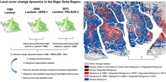
Graphical Abstract

1. Introduction

Deltas are economic and environmental hot spots [1]. They take up less than 1% of the Earth’s surface but are home to more than ca. 7% of the global population—a density more than 10 times the average [2]. Deltas are able to support such high human populations thanks to the high productivity, biodiversity, and the ability to use the waterways for transport. They are key contributors to the production of agricultural goods and are, therefore, highly important in the fight against global food insecurity [3]. However, these important systems are highly delicate and vulnerable. Tropical delta regions, in specific, are under risk of numerous threats, including sea level rise, extreme floods, storm surges, erosion, subsidence, and salinity intrusion, amongst others, which are expected to increase both in frequency and magnitude with the climate crisis [4]. These problems have been proven to increase out-migration rates and human security risks in developing regions, often inhabited by some of the poorest populations in the world [3]. Given the importance and the vulnerability of tropical deltas, monitoring and understanding the land cover dynamics in these regions is vital for achieving efficient policy planning and progress toward achieving the Sustainable Development Goals [5].
The Niger River Delta (NRD) is the largest river delta in Africa [6] and home to a rapidly increasing human population. It features the largest mangrove forest in Africa, estimated to be ~5% of the global mangrove coverage and the fifth largest mangrove forest in the world [7]. It is recognised as a highly important resource for the local communities, as it is utilised for fisheries, fuelwood, construction material, flood protection, medicinal purposes, recreation, and tourism, and holds an important spiritual value [8,9,10,11,12,13]. Substantial oil and gas deposits are found under the mangrove ecosystem of the NRD. Over the last decades, this highly significant ecosystem is under threat of loss or degradation, mainly due to oil and gas exploration activities, the overexploitation of the mangroves for fuelwood, urbanisation, and the invasion of the Nipa palm species (Nypa fruticans) [11,14,15,16,17,18,19]. Climate change [13,20], sea level rise [21], and coastal erosion [22] are also threats to the mangrove system. Despite the importance of the NDR resources, and the perceived degradation from anthropogenic and environmental pressures, reliable information on land cover dynamics and, particularly, on the extent and condition of the mangrove forest, is still lacking.
Assessing land cover dynamics over large areas is only possible via Earth Observation technologies, which is commonly done with multi-temporal Landsat data. The Landsat archive is truly invaluable as it constitutes the only global medium-scale data available for ~50 years. More ‘traditional’ approaches have used image mosaics or single images from single-sensor data to map two (before and after) dates and assess change from these [9,23,24,25,26,27]. However, over certain parts of the world, e.g., western and eastern Africa, the data archive has significant gaps [27,28]. Moreover, the use of optical data for accurately mapping and monitoring land cover dynamics over the tropics can be problematic due to the extensive cloud contamination, which renders the creation of image mosaics over large areas an unachievable task [29,30,31].
Recent advances in data availability, computing power, cloud computing, and algorithm development (e.g., machine and deep learning) have given rise to new approaches to multi-temporal assessments of land cover, e.g., image compositing [32], and spectral-temporal metrics [33,34]. The combination of optical and radar data has also been hailed as an important advancement in regional-scale land cover mapping as certain land cover types, such as mangroves and savannah woody vegetation, are mapped successfully using radar backscatter data, taking advantage of their ability to ‘see’ through cloud [19,35,36,37,38,39,40,41]. Over the last decade, object-based image analysis (OBIA) approaches have also been tested to successfully separate mangrove species from other coastal vegetation [42], to map the Amazonian mangrove belt [38], and to assess long-term variations of forest loss, fragmentation, and degradation using a combination of OBIA and spatial autocorrelation indicators [43].
There has been a limited number of studies that mapped land cover dynamics in the NDR [9,23,27,44] as the area is one of the most affected worldwide from the gaps in the Landsat archive and a consistent cloud contamination. With the exception of Nwobi et al. [19], these have employed ‘traditional’ remote sensing approaches and results have been contradictory. Even fewer studies have attempted to estimate the spatial extent of the degraded mangrove cover. Kuenzer et al. [27] used mosaics of Landsat images to map land cover change in the NDR over three dates but reported low per class classification accuracies for both the “tall mangrove” and the “degraded mangrove” classes, making area calculations unreliable. Salami et al. [45] compared the accuracies achieved by using Landsat ETM+, ASTER and NigeriaSat-1 data to map the six main land cover classes. For the mapping of degraded mangrove, they reported high accuracies for all three platforms. However, their study covered a small fraction of the NRD.
Based on the initial assessment of land cover transitions and dynamics, land cover change studies often move on to explain the changes in terms of explanatory variables (i.e., land use change drivers) or to forecast spatial patterns of future land cover under different scenarios (i.e., land use change models) [46,47,48,49,50,51]. The success of these next stages greatly depends on the ability to carry out an accurate initial assessment of the dynamics. Moreover, apart from the need to map land cover accurately, there is also a requirement to understand the dynamics more fully. For example, a simple comparison among the land cover maps does not determine whether the observed changes derive from processes that are systematically more intensive than random processes. Over the last years, new approaches have been suggested for characterising land cover change patterns quantitatively so that any potential subsequent analyses can focus more efficiently on the important patterns and processes of change, such as the intensity analysis proposed by Aldwaik and Pontius [52]. Other studies, with a specific interest on the fragmentation of habitats for example, have focused on the calculation of landscape metrics from the initial assessment of land cover. These studies have shown that the fragmentation of forests has detrimental effects for the health of the ecosystem and the services that it is able to provide [50,53,54]. A number of indices have been created to quantify landscape structure and spatial heterogeneity based on the composition and configuration of the landscape [55,56,57,58].
To date, no study related with the assessment of land cover change in the NDR has incorporated recent analytical approaches (e.g., intensity and fragmentation analyses) and the technological and algorithmic achievements (e.g., multi-sensor data, machine learning algorithms) to improve classification accuracies and our understanding of the land cover dynamics. Therefore, there is a need for a comprehensive study of land cover change in the region. In this paper, we aim to accurately assess the land cover dynamics in the NDR over the last decades, and improve our understanding of the extent of the degradation of the delta’s mangrove forest. We will do so by:
  • Mapping the main land cover types of the NDR in three epochs using Landsat data, spectral-temporal metrics, and a machine learning algorithm;
  • Testing the performance of the classifier when radar L-band data are added to the Landsat;
  • Assessing land cover change intensity over the two periods; and
  • Quantifying the mangrove forest degradation and its fragmentation using landscape metrics.

2. Study Area

The Niger Delta is a flat alluvial plain located in Nigeria on the Gulf of Guinea (Figure 1). It is the largest river delta in Africa formed primarily by sediment deposition. It has a coastline of 470 km and consists of a number of ecological zones, including mangrove swamps, freshwater swamps, forests, and lowland rain forests. The Delta has two distinct seasons (wet and dry) with an average temperature of 27 °C throughout the year and annual rainfall of 3000 to 4500 mm [13]. The Niger Delta Region covers an area of 56,000 km2 that consists of 7 administrative states (Abia, Akwa Ibom, Anambra, Bayelsa, Delta, Imo, and Rivers) and is home to more than 33 million inhabitants (265 people per km2; [59]). More than 70% of these people depend on the natural environment for their livelihoods.
The NDR is considered a hot spot for biodiversity in the world with 3 sites designated as Ramsar Wetlands of International Importance [60]. It is a hub for oil and gas exploration, home to 80% of the refineries in Nigeria and extensive infrastructure (e.g., c. 900 oil wells, c. 100 flow stations and gas plants, c. 1500 km trunk lines, and c. 45,000 km flow lines) [61]. Nigeria’s GDP, which rose from ~292 billion USD in 2009 to over 448 billion USD in 2019 [62], is mainly generated by the oil and gas sector. Yet, the NDR remains under-developed and its inhabitants impoverished. The Nigerian Land Use Act excludes the ownership of oil minerals by the state. This is perceived by many as socially inequitable, and has resulted in continuous instability in the region [63]. Additionally, more than 220 oil spills and 17 billion cubic metres of gas flares per year, together with the impacts of the human population explosion, have led to the degradation of the Niger Delta ecosystem [9,10,19,27,64].

3. Materials and Methods

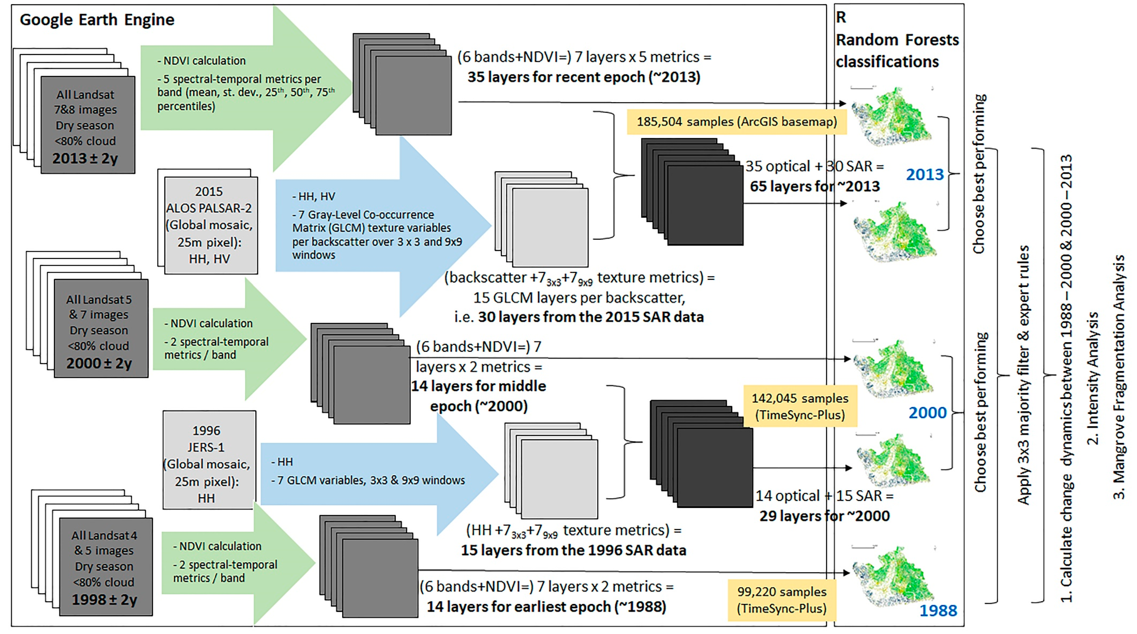
We mapped the main land cover types in three epochs centred around 1988, 2000, and 2013, and assessed land cover change and change intensity in the two respective periods. The chosen classes were: Water, urban (i.e., built-up), woodland (i.e., lowland rainforest and freshwater forest), bareland, agricultural land, grassland, mangroves, and degraded mangroves. The choice of the classes was based on our knowledge of the area, the nomenclature used by ESA’s 20 m land cover data for Africa and the 30 m-pixel Landsat-based GlobeCover30, and our desire to separate healthy mangroves from degraded ones. By definition, degraded is the land that has temporarily or permanently undergone a lowering of its capacity to deliver ecosystem services [65]. In the case of mangroves, the degraded forest has less biomass and tree cover, and is unable to provide a number of services at the same level as the healthy system, e.g., support for local livelihoods, carbon sequestration, erosion protection, provision of habitat for numerous fauna species, amongst others [66]. We also assessed the fragmentation of the mangrove forest during these two periods. Additionally, we tested the performance of the classifier when radar data are added to the optical. Figure 2 is a flowchart of our methodological framework.

3.1. Data

3.1.1. Reference Data

Very high-resolution reference data were used for the recent epoch. This dataset is available as a MAXAR Vivid basemap within the ArcGIS software [67,68]. These cover the study area with data from November 2009 to January 2017. About 90% of the study area is covered with 46-cm-pixel data from GeoEye-1 (10 December 2010, 16 December 2011, 3 January 2013, 17 December 2013, 10 April 2014, 8 January 2015), 60-cm-pixel data from QuickBird-2 (11 February 2010, 3 October 2010, 12 June 2013), and 50-cm-pixel data from WorldView-2 (1 December 2011, 16 February 2013, 13 January 2014, 12 March 2015, 17 December 2015). Thanks to the familiarity with the study area, the broad land cover classes that were targeted in this paper were relatively easily identifiable on the very high-resolution imagery. This was also the case for the degraded mangroves, which presented the additional advantage of being spatially confined within the coastal zone, in general, and the mangrove system, in particular.

3.1.2. Landsat Data

The choice of Landsat data was driven by the need to coincide with as many other NDR studies as possible, so that comparisons could be drawn between them. Two such studies were identified: the one by Ayanlade and Drake [23] and the study by Kuenzer et al. [27]. The latter was particularly targeted, as it is the only one that has attempted to map the “degraded mangrove” class. The choice of the three epochs was also driven by the availability of the reference data and the SAR imagery.
We used all the dry season (December to February) Level 1 surface reflectance Landsat 4, 5, 7, and 8 images centred around 1988 (±2 years), 2000 (±2 years), and 2013 (±2 years) with less than 80% cloud cover from the USGS EROS Data Center for the eight WRS-2 tiles covering the study area (path 187, row57; p188, r55; p188, r56; p188, r57; p189, r55; p189, r56; p189, r57; p190, r56). Only the non-thermal bands were used, and clouds and cloud shadows were removed using F-mask [69,70]. Finally, the Normalised Difference Vegetation Index (NDVI) [71] was calculated. From the resulting 7-band image stacks (i.e., six non-thermal bands, plus the NDVI), spectral-temporal variability metrics were calculated [33,34,72,73]. For the recent epoch, five statistics for each of the seven bands were calculated: the standard deviation, the mean, and 3 percentiles (25th, 50th, and 75th). This brought the total layers for this epoch to 35. However, as data availability for the first two epochs was problematic (Figure 3), we limited the number of statistics per band to 2 (mean and st. dev.) and the total number of layers to 14.

3.1.3. Radar Data

Radar data were chosen for testing whether their addition to the optical metrics could improve the land cover classification. For the recent epoch, we employed the 2015 global 25 m resolution L-band Synthetic Aperture Radar data from the Advanced Land Observing Satellite-2 (ALOS-2) PALSAR-2 sensor via Google Earth Engine’s API. The data are free and open access with two polarisations (HH and HV) and are currently available for 2015 to 2018. To increase the utility of the SAR data, we used Google Earth Engine to calculate a series of Gray-Level Co-Occurrence Matrix (GLCM) texture variables [72]. GLCMs are a series of localised texture metrics that quantify the statistical properties of a layer over a moving window [74]. We calculated seven GLCM layers (mean, variance, homogeneity, contrast, dissimilarity, entropy, and second moment) [75]. These statistics were calculated over both 3 × 3 and 9 × 9 windows, resulting in 15 layers per SAR backscatter (one backscatter + seven 3 × 3 GLCM layers + seven 9 × 9 GLCM layers), totalling 30 layers for the year 2015.
For the middle epoch, we acquired JAXA’s 25 m resolution JERS-1 tropical region mosaics for the year 1996, the only year that such data are available over the Niger Delta Region. One polarisation is available (HH), from which we calculated 15 GLCM layers to use in the classification.

3.2. Land Cover Mapping

3.2.1. Sampling and Validation

In total, 185,504 samples were taken for the epoch centred around 2013. For the first and second epochs (i.e., 1988 and 2000), TimeSync-Plus v4.6 was used [76] to check for unchanged pixels at the 2013 sample locations. This resulted in 142,045 and 99,220 samples, respectively, for which we could confidently say that no change in the Landsat time series occurred. During classification, half of these samples were used for training and half for validation.

3.2.2. Image Classification & Post-Classification Processing

We developed the land cover classification using Random Forests classification models. Random Forests have been used successfully to classify Landsat imagery, thanks to their effective handling of correlated predictors and reduced tendency toward overfitting [77]. We used the ‘RStoolbox’ and ‘randomForest’ packages within the R statistical environment [78]. One optical only model was tested for the first epoch, while for the middle and most recent ones, we tested the performance of optical only and optical + SAR metrics (Figure 2). Based on the accuracies achieved, the outputs from the best performing models were chosen for the middle and more recent epochs. A 3 × 3 majority filter was applied to the outputs from all 3 epochs to get rid of the ‘salt and pepper’ effect of the classification. Finally, based on our knowledge of the study area, expert rules were applied to correct for some classification errors [72].

3.3. Intensity Analysis

Aldwaik and Pontius [52] devised a methodology that characterises patterns of land change quantitatively. It provides a mathematical framework that compares a uniform intensity to observed intensities of temporal changes among land cover classes (or ‘categories’) [79]. There are three levels of analysis, with each level exposing different types of information given the previous level of analysis. The first level, i.e., the interval level, examines how the size and speed of change vary across time intervals. The intensity of the rate of annual change is estimated using the following equations [52] (for notation, see Table S1 in the Supplementary Material):
S t = a r e a   o f   c h a n g e   d u r i n g   i n t e r v a l   [ Y t   ,   Y t + 1 ] / a r e a   o f   s t u d y   r e g i o n d u r a t i o n   o f   i n t e r v a l   [ Y t   ,   Y t + 1 ]   ×   100 % ,
U = a r e a   o f   c h a n g e   d u r i n g   a l l   i n t e r v a l s / a r e a   o f   s t u d y   r e g i o n d u r a t i o n   o f   a l l   i n t e r v a l s   ×   100 % .
The second level is called “category level” and it examines how the size and intensity of gross losses and gross gains in each land cover class vary across classes for each time interval. This level identifies which land cover classes are relatively dormant or active in each time interval [52]. Equations (3) and (4) provide the intensity of a class’ annual gain and loss, respectively:
G t j = a r e a   o f   g r o s s   g a i n   o f   c l a s s   j   d u r i n g   [ Y t   ,   Y t + 1 ] / d u r a t i o n   o f   [ Y t   ,   Y t + 1 ] a r e a   o f   c l a s s   j   a t   t i m e   Y t + 1   ×   100 % ,
L ti = a r e a   o f   g r o s s   l o s s   o f   c l a s s   I   d u r i n g   [ Y t   ,   Y t + 1 ] / d u r a t i o n   o f   [ Y t   ,   Y t + 1 ] a r e a   o f   c l a s s   i   a t   t i m e   Y t   × 100 % .
The third level, the “transition level”, examines how the size and intensity of land cover class’ transitions vary across the other classes that are available for that transition [52]. At each level, the method tests for stationarity of patterns across time intervals and identifies which land cover transitions are particularly intensive in a given period. Aldwaik and Pontius [52] provide a detailed explanation of the limitations concerning where the transition from a particular land cover class m to a class n can occur. For example, if a given land cover class n exists at a particular location at the initial time, then class n cannot gain at that place. If class n gains, then it must gain from locations that, initially, are not class n. If class n gains uniformly across the study area, then this class will gain from other classes, in proportion to the initial sizes of these land cover classes. Alternatively, class n might intensively avoid gaining from some particular class(es) and might intensively target gaining from some other class(es). Given the observed gross gain of class n, Equations (5) and (6) identify which other classes are intensively avoided versus targeted for gaining by class n in a given time interval:
R t i n = a r e a   o f   t r a n s i t i o n   f r o m   i   t o   n   d u r i n g   [ Y t   ,   Y t + 1 ] / d u r a t i o n   o f   [ Y t   ,   Y t + 1 ] a r e a   o f   c l a s s   i   a t   t i m e   Y t   ×   100 % ,
W tn = a r e a   o f   g r o s s   g a i n   o f   c l a s s   n   d u r i n g   [ Y t   ,   Y t + 1 ] / d u r a t i o n   o f   [ Y t   ,   Y t + 1 ] a r e a   t h a t   i s   n o t   c l a s s   n   a t   t i m e   Y t   ×   100 % .
We used the intensity.analysis package in R to carry out the processing (https://cran.r-project.org/web/packages/intensity.analysis/vignettes/README.html).

3.4. Landscape Pattern Analysis

Post-classification comparison is most informative about changes in the composition of a landscape but gives us little—only visual—information about the spatial characteristics of these changes and the distribution of landscape elements. Landscape pattern analysis using landscape metrics provide us with additional information about the structure of changes, such as landscape fragmentation and patch aggregation or dispersion, as well as their changes in time. With the latter, we can observe changes in landscape spatial configuration through time.
We followed the approach used by Gounaridis et al. [53] and selected a number of class-level metrics [80] in order to study the changes in the spatial configuration and patterns of the ‘mangrove’ and ‘degraded mangrove’ land cover classes. We used ‘Percentage of Landscape’ (PLAND) as a measure of class abundance, and the ‘number of patches’ (NP), ‘landscape patch index’ (LPI), and ‘patch area median’ (AREA_MD) to study fragmentation of the classes of interest. With regard to patch shape analysis, we used the ‘area weighted mean patch shape index’ (SHAPE_AM), and for the aggregation of these classes, we used the ‘area weighted mean Euclidean nearest neighbour distance index’ (ENN_AM) along with its standard deviation (ENN_SD). Finally, we also used the aggregation index of ‘percentage of like adjacencies’ (PLADJ). Table 1 provides a listing of the selection of landscape metrics used in this study, together with a short description of their correlation with mangrove forest fragmentation. For more information, refer to McGarigal and Marks [80] who provide a full description of the metrics, including their mathematical formulas.

4. Results

4.1. Land Cover Mapping and Validation

Figure 4a–c are the outcomes of the classification of the metrics for the three epochs, and are accompanied by pie charts that summarise the proposition covered by each class. For the middle and latest epochs (Figure 4b,c), the combination of the optical with the SAR data produced slightly better results (Table 2) and were, therefore, the ones chosen for the subsequent analyses. The largest land cover class is by far woodland, which covers ~40% of the area (~23,000 km2). Agricultural land is the second largest in all three time points (~12,000 km2), while mangroves (degraded and non-degraded) and grassland occupy significant portions of the delta, too (~8000 km2).
The classification results produced high overall accuracies of 79% (95% CI: ±3%), 83% (95% CI: ±3%), and 82% (95% CI: ±2.6%) for the three epochs, respectively (Table 2). Per-class accuracies (% correct, producer’s and user’s Accuracies; Table 2) were also high, with the exception of the bareland and grassland classes. The lower accuracies for these two types are attributed to the spectral confusion with the agricultural class: when fields are fallow, it gets confused with bareland, while when they are covered with vegetation, it is mostly confused with grassland (Tables S1–S5). The latter is also confused with woodland, as open woodland pixels contain a significant amount of spectral response from grasses.
Most importantly for the objective of this study, the mangrove class was mapped with high accuracy, with percentage correct and user’s and producer’s accuracies above 90% in all three time steps and models (Table 2). The degraded mangrove class was also mapped accurately, with producer’s accuracies being consistently very high for all epochs and data combinations. However, there was some confusion between this class and the non-degraded mangroves (confusion matrices Tables S2–S6 in the Supplementary Material), resulting in lower user’s accuracies, ranging from 77% to 79% for the first two time points (Table 2).
The inclusion of the SAR data in the classification of the more recent epochs generally improved the results but only slightly (Table 2). The most noteworthy improvements were achieved by the inclusion of the PALSAR-2-based metrics in the latest time point, with the user’s accuracies of the water and urban classes improving by 4% (Table 2).

4.2. Land Cover Change Dynamics

The three land cover maps were used to calculate the contingency matrix in Table 3. The matrix summarises, for the two periods, the area that has remained unchanged and the area and the type of change observed for each individual class. It also provides a summary of the area covered by each class in the beginning and in the end of each period as well as of the gains and losses they experienced. The spatial distribution of the latter is also illustrated in Figure 4d–g.

4.3. Intensity Analysis

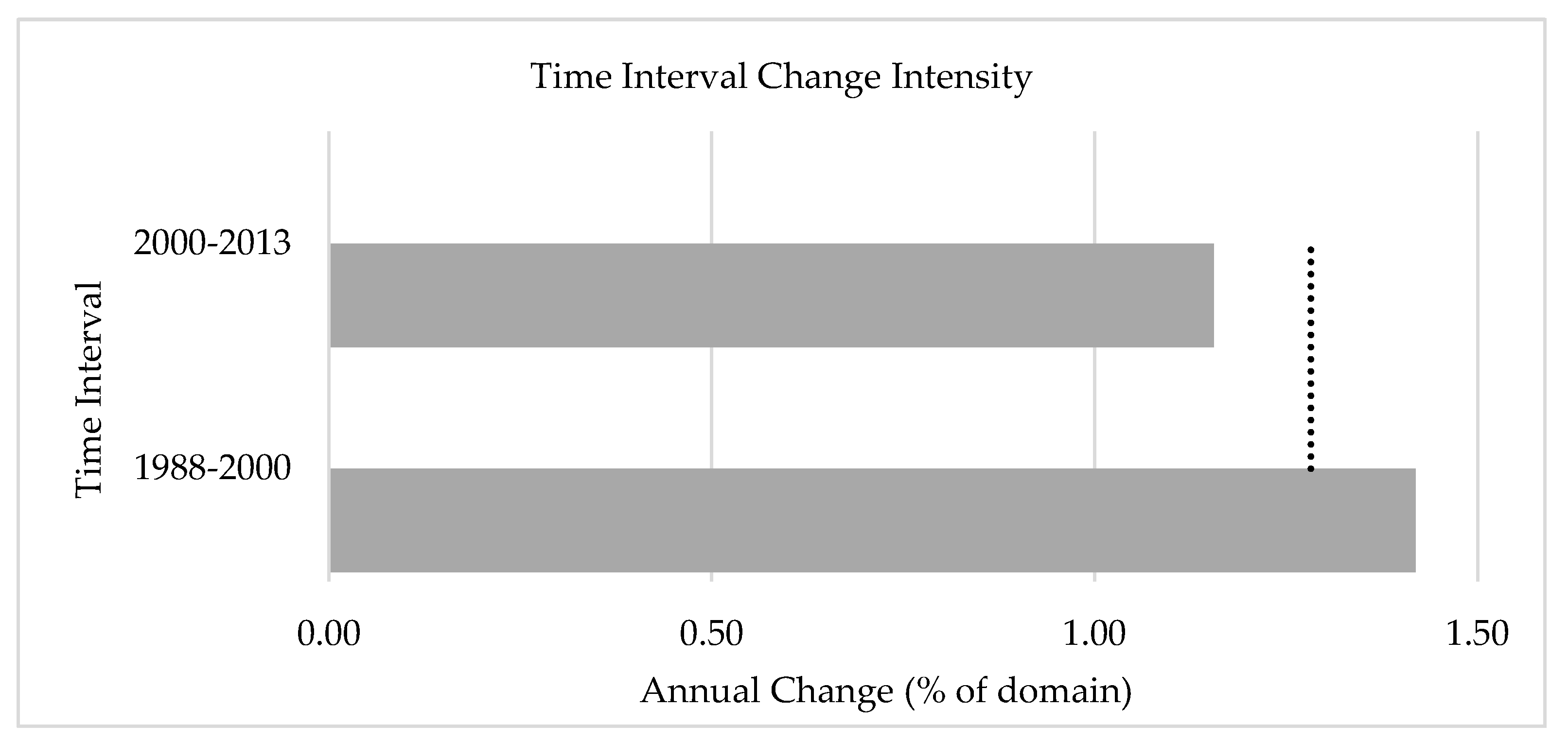
The interval level of the intensity analysis identifies the time interval in which the overall annual rate of change is faster. The total change in both intervals was found to be relatively similar: ~17% of the total area in the first period and ~15% in the second. However, the intensity of the annual area of change in the first interval is faster than in the second (1.42% and 1.16%, respectively; Figure 5). The output of Equation (2) is 1.28%, depicted as a dashed line in Figure 5. Compared to this value, the rate in the first period is considered ‘fast’, while in the second ‘slow’.
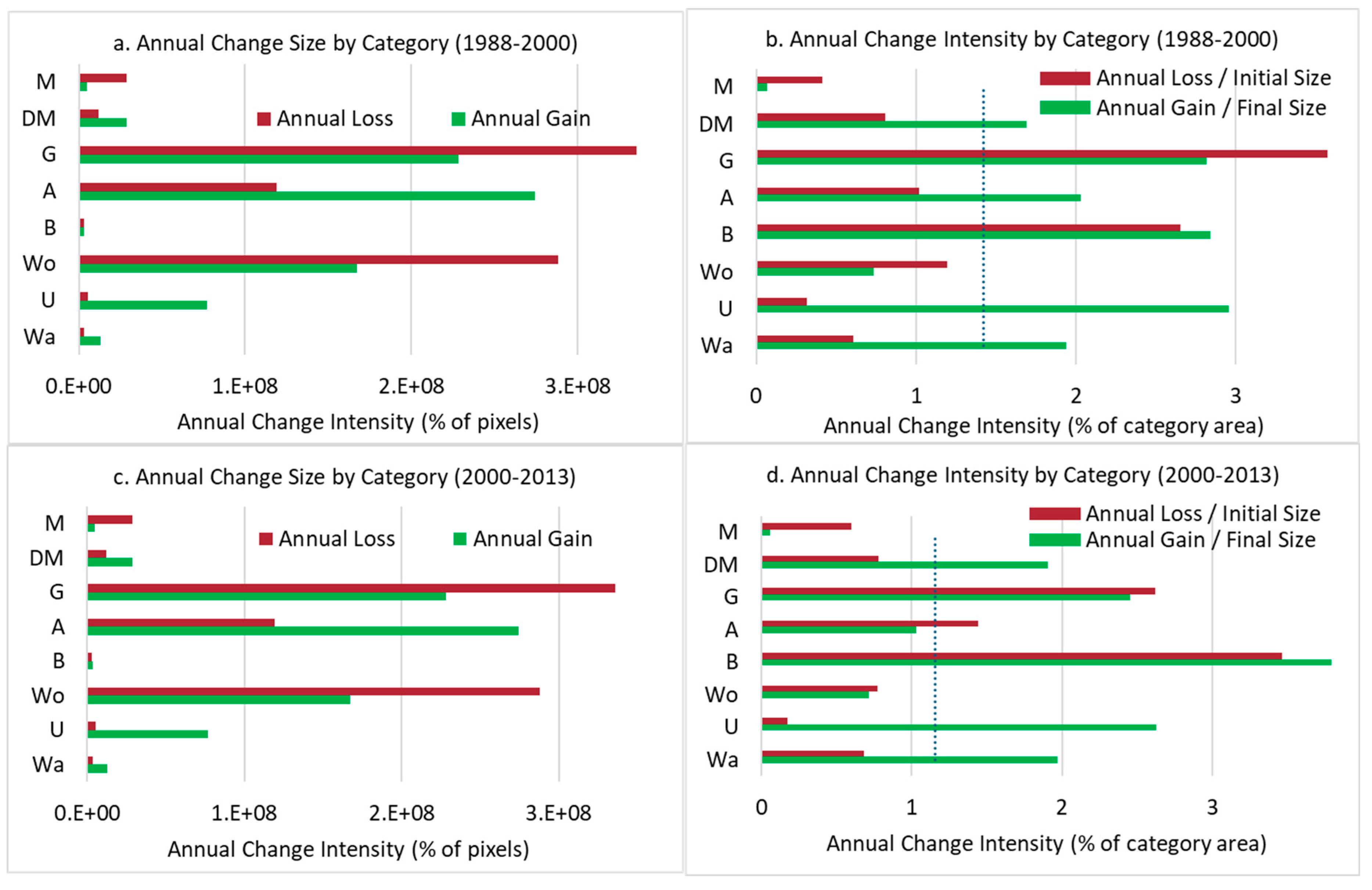
Figure 6 is the graphical representation of the ‘category level’ of the intensity analysis. Figure 6a,c depict the size of the annual gain of loss of each land cover class in the first and the second period, respectively. Figure 6b,d show the intensity for a class’ annual gain or loss, as calculated by Equations (3) and (4). The two dashed lines show the output of Equation (1) for each period, i.e., the uniform line for each period at this category intensity level [52]. When an intensity bar remains to the left of the uniform (dashed) line, then the change is relatively dormant for that land cover class and period. On the contrary, if the bar extends to the right of the dashed line, then the change is relatively active for that class and period. If, for a given land cover class, the intensity of the gains or losses remain active or dormant during all study periods, then the specific type is considered stationary.
At the transition level, the intensity analysis identifies which transitions are more intensive in a given time interval. Given the scope of the present paper and the need to keep the presentation of the results as succinct as possible, Table 4 summarises the results only for the transition from mangrove to any other class for the two periods. The outcome for all the other transitions is provided in Tables S7 and S8 of the Supplementary Material.

4.4. Landscape Pattern Analysis

Figure 7 depicts the evolution of the selected landscape metrics through time for the healthy and the degraded mangroves classes.

5. Discussion

Accurate and reliable information of land cover dynamics is essential for the sustainable management of tropical deltas and mangrove ecosystems and their capacity for ecosystem service provision. The ‘traditional’ remote sensing mapping approach involving the use of image mosaics of optical data from two dates, together with likelihood function maximisation image classification algorithms, is not reliable in the humid tropics due to cloud cover [29,31], data availability [27,28], and algorithm performance. This has led to conflicting land cover change estimates for the largest river delta in Africa and the failure to assess the extent of degradation of one of the most endangered ecosystems in the world [60]. Our results show that, by incorporating novel image compositing techniques, spectral-temporal metrics, and machine learning classification algorithms, a reliable assessment of the change dynamics over the Niger Delta Region can be made. Our accurate land cover estimates also allowed for a more comprehensive land change analysis that incorporates an assessment of change intensity and the fragmentation of a key component of the NDR: its mangrove forests.

5.1. Land Cover and Change Dynamics

There is an inherent difficulty in mapping land cover in tropical deltas, in general, and mangrove forests, in particular, as they are affected by seasonal and intertidal effects, with pixels often comprising of a mixture of vegetation, soil, and water due to their location between land and sea and the average tidal range in the Niger Delta being 1.5 m [9]. Nevertheless, we mapped the eight main land cover types for the entire NDR, achieving high overall accuracies in all epochs (~79% for 1988, and 82% for 2000 and 2013; Table 2) and high producer’s accuracies for all classes and years. With the exception of the grassland and bareland classes, user’s accuracies were also high (from 70% to 91%). Our results compare favourably with other studies in the NDR [19,23,44,45]. Regarding the mapping of degraded mangroves, one of the main objectives of this paper, our study is the first to map this accurately with user’s accuracies between 77% and 87% and producer’s consistently above 82%. The only other study that attempted to map degraded mangroves reported very low accuracies [27].
The results reveal some interesting dynamics:
  • There is consistent net loss in mangrove and woodland types and a consistent net gain of the urban class in both periods of study
  • The area covered by non-degraded mangroves was reduced by ~250 km2 in each period (=Gross Loss – Gross Gain)
  • About 10% of mangroves are degraded in each interval, and an additional 34 km2 of mangrove were converted to urban land use in both periods
  • A portion of degraded mangrove is able to bounce back into its healthier state
  • The net loss for the woodland class was more than 700 km2 in each period. A part of this class is converted to grasses (~8% and ~9%) and to agricultural land (~7% and ~5%)
  • A quarter of the area mapped as grassland in the initial dates is converted to woodland by the end date
  • The built-up areas increased by 47% (~900 km2) in the first period, an area larger than the size of New York City. In the second period, the increase was smaller (~800 km2) but still it amounted to 27% of the area covered in 2000
More specifically, according to our findings, healthy mangroves reported a net loss in both study periods: 292 km2 in the first and 235 km2 in the second, while degraded mangroves consistently reported a net gain (21 km2 in the first and 97 km2 in the second). Interestingly, our study and the studies by Kuenzer et al. [27] and James et al. [9] found a similar decrease in the overall combined (degraded and non-degraded) mangrove area. According to our results, this area was 270 km2, while, in an almost identical period of study, Kuenzer et al. [27] found that the loss was 239 km2. In the James et al. [9] study between 1987 to 2002, the loss was 213 km2. However, our more accurate findings identify the total areas covered by the mangrove classes to be very different to the areas in the Kuenzer et al. [27] study: we found that mangroves and degraded mangroves occupied an area between 8697 and 8428 km2 in the two periods, while Kuenzer et al. [27] claim that these numbers were 10,311 and 10,072 km2, respectively. These figures differ by almost a fifth, and can play a significant role in the setting of conservation targets, management policies, and sustainability goals. Moreover, our mangrove results compare favourably with three studies that mapped mangroves as one class accurately: the study of Nwobi et al. [19], who found that mangroves occupied an area of 9115 km2 in 2007 and 8017 km2 in 2017; the study of Ayanlade and Drake [23] (9965 km2 in 1987, 9255 km2 in 2001, and 8430 km2 in 2011); and the study by James et al. [9] (7037 km2 in 1987 and 6824 km2 in 2002).
While it is relatively simple to compare the results on the extent of mangroves between the different studies that mapped land cover change in the NDR, as this class is confined in the coastal belt and is always included within the study area, it is not as straightforward to compare the findings on other land cover types, as the study areas do not match. In the case of woodland, for example, the biggest land cover type in the NDR, our study found that it occupied 23,770 km2 in 1987 and suffered net losses in both periods: ~700 km2 in the first and ~800 km2 in the second. The study by Ayanlade and Drake [23] also found net losses in both periods for the combined “lowland rainforest” and “freshwater forest” classes but found that these occupied 31,200 km2 in 1987, 25,400 km2 in 2001, and 21,470 km2 in 2011. However, their study area far exceeds the boundaries of our delineation of the NDR. The study by Kuenzer et al. [27] also agrees that “forest” and “swamp forest” experienced net losses in both periods. They report far smaller areas than both our study and the study by Ayanlade and Drake [23]: 18,325 km2 in 1987 and 15,408 km2 in 2013. Finally, the Nwobi et al. [19] study also agrees that “tropical forests” were reduced but reported that these occupied 29,000 km2 in 2007 and 25,500 km2 in 2017. As all of these studies, including ours, reported high per-class accuracies in the mapping of forests, it is difficult to ascertain which on is closer to the true figure.
The difficulty in comparing the findings of different studies remains for the agricultural class, which we found to significantly increase in the first period (from 11,571 to 13,787 km2) and decrease in the second (12,645 km2 in 2013). An additional issue to the problem of relating to different study areas around the NDR is the choice of land cover nomenclature. Based on our knowledge of the region and on the classification systems of the ESA 20m African land cover data for 2016 and the GlobeLand 30 m data for 2010, we included a grassland class in our mapping efforts, which were found to decrease in the first period (from 9421 to 7089 km2) and increase in the second (8102 km2 in 2013). Our figures for the agricultural class are significantly lower to those in Ayanlade and Drake [23], Kuenzer et al. [27], and Nwobi et al. [19]. However, none of these studies included a separate class for grassland but, according to their spatial outputs, appear to have mapped this together with the agricultural class. We recognise that separating these classes poses difficulties, as the spectral separability between them is low: our user’s accuracies for grassland are testament to that (Table 2). However, we strongly believe that it is a shortcoming to map these two classes as one, as this precludes the identification of very important land cover dynamics between either of these classes and, for example, the woodland or urban classes. If summed together, our estimates of agricultural and grassland compare favourably with those of Nwobi et al. [19], who estimated the area covered by “agricultural land” as 21,733 km2 in 2007 and 24,179 km2 in 2017.
An important change that occurred in both periods is the expansion of the built-up areas: from 1990 km2 in 1988, to 2924 km2 in 2000, to 3728 km2 in 2013, i.e., an 87% increase. As in the previous land cover types, the difference in the extent of the study area makes comparison to the other studies difficult. For example, the Ayanlade and Drake [23] study reports much higher figures, but their study includes the city of Benin, the fourth largest Nigerian city, which lies outside of our delineation of the NDR. Similarities exist between our findings and the Nwobi et al. [19] study: their ‘built-up-area’ class occupied 3950 km2 in 2007 and 5938 km2 in 2017. Their higher estimates can be attributed to the fact that they include the city of Calabar and a number of built-up areas in the northeast of their study area that lie outside our delineation of the NDR.
According to the results of our intensity analysis (Figure 6b), in the first period of study, only mangroves and woodland demonstrated dominant gains, while all the other categories had active gains. Interestingly, only the grassland and bareland types had active annual change intensities, with the former having the largest size of losses in this period (Figure 6a). However, these two are the classes that scored lower user’s accuracies and the respective intensity results need to be treated with caution. Notable results from this period are the ~5 times greater annual intensity of mangrove loss than gain and the ~10 times greater annual intensity of urban gain than loss. The intensity of agricultural expansion is also noteworthy, reporting ~2 times greater gain than loss.
In the first period, the land cover class that mangroves ‘target’ most intensively when they change is degraded mangroves, with a transition intensity of 1.57% of the total area of degraded mangroves in the end of the first period. This is much higher than the estimated uniform change intensity of 0.06%. An area of 535 km2 of mangroves was degraded by the year 2000. In the second period, this change is even more intense (1.80%, higher than the uniform intensity of 0.08%) and leads to a conversion of a total of 596 km2 of mangrove to degraded mangrove by 2013. Bareland is also found to be a targeted class for mangroves with an estimated transition intensity of 0.20% (221 km2). Water also targets bareland, as well as mangroves and degraded mangroves, with transition intensities higher than the estimated uniform change intensity. As this is the first paper to undertake an intensity analysis in the NDR, we are unable to compare our findings to existing studies.

5.2. Fragmentation and Degradation of the Niger Delta Mangrove Forest

The Niger Delta’s mangrove forest is a hub for substantial oil and gas deposits. As a consequence, it is highly vulnerable to activities of oil and gas extraction, e.g., land clearing, dredging, construction of flow stations, pipe and seismic lines, well blowouts, leakages or corrosion, equipment failure, error during operation or maintenance, accidents during transportation, sabotage, etc., as well as urbanisation, selective logging, and the proliferation of the invasive Nipa palm species (Nypa fruticans) that lead to the forest’s destruction, fragmentation, and degradation [9,10,19,27,64].
Our land cover change and intensity analyses showed that degraded mangroves increased in both periods of study and mangroves losses were 5 times more intense than gains. To further assess the condition of the Niger Delta mangrove forest, we carried out the first ever fragmentation analysis of the area. Our fragmentation results show that the ‘number of patches’ (NP) for the healthy mangroves increased persistently while the ‘total percentage of landscape’ (PLAND) decreased (Figure 7a,b). The ‘largest patch index’ (LPI), a measure of dominance (Figure 7c), shows that in the second period, larger patches are on a decrease. The ‘area weighted mean shape index’ (SHAPE_AM; Figure 7f) is also decreasing for the healthy mangroves, in both periods: this indicates that changes are happening in the perimeter of patches, uniformly. The ‘area weighted mean Euclidean nearest neighbour distance’ index (ENN_AM; Figure 7d) is slightly decreasing, indicating less dispersion of the healthy mangrove patches. The standard deviation of this index (ENN_SD; Figure 7h) is decreasing but with high values compared to the mean, which indicates a more uneven distribution of patches. The high and steady values of PLADJ (Figure 7g) confirm the ENN results: the healthy mangrove patches remain relatively aggregated throughout the study period. This was expected, as mangroves are very localised within the delta and naturally only occur by the coast.
Figure 7 also shows the change in landscape metrics through time for the degraded mangroves. The size of this class (PLAND; Figure 7a) is constantly increasing but shows some fluctuation in the number of patches (NP; Figure 7b). A divergent pattern is observed in the evolution of the number of patches and the median of patch area metrics (AREA_MD; Figure 7e): NP increases in the first period and AREA_MD decreases, while in the second period, this is reversed. The latter means that this class becomes less fragmented, with more patches and lower patch size in the first period. Between 2000 and 2013, there are fewer patches and larger patch sizes, indicating that some of the first period’s patches have merged to form larger ones.
A visual examination of the land cover maps and derived change maps from these revealed three areas that demonstrate higher concentrations of degraded mangrove. One such area is in the eastern part of the NDR, around the city of Port-Harcourt and the towns of Bonny, Okrika, and Degema (Figure 8a). Mangrove degradation here can be attributed to the effects of rapid urbanisation and oil extractive activities [14,17], as demonstrated by the overlap with the locations of the oil wells, the pipelines, and the oil spills in Figure 8a. At the central part of the study area, mangrove degradation is mainly due to oil spills resulting from crude oil extractive activities, notably near River Bayelsa and the towns of Nembe, Southern Ijaw, Ekeremor, Brass, and Oloibiri, where oil extraction first began as early as the 1950s (Figure 8b). The highest concentration of degraded mangroves is, however, in the western part of the NDR, in the Delta state (Figure 8c). This area shows widespread degradation, with a notable increase in the second and third date around the towns of Wari South and Wari South West. Several oil spill and gas incidents have been reported in the literature around this area and period [14,15,17,18].

6. Conclusions

The Niger Delta Region (NDR) is an important ecosystem, providing numerous services to the millions of its human inhabitants. Despite its undisputable importance, it is under threat of degradation, mainly due to human pressure, and especially as a direct consequence of the activities related with the significant oil and gas reserves in the region. Understanding the extent of the problem requires an accurate assessment of the land cover dynamics in the region, which can only be achieved through the use of state-of-the-art remote sensing technologies and analytical techniques. Cloud contamination and gaps in the commonly employed Landsat archive makes this a fathomable task.
Here, we were able to accurately assess the land cover dynamics over a period of 25 years using the Google Earth Engine cloud computing platform to estimate spatial-temporal Landsat-based metrics in three epochs. Our results showed that mangroves, the lowland rainforests, and the freshwater forests have demonstrated a net loss, while the built-up areas have almost doubled in the period of study. By performing a land cover change intensity analysis, we were also able to demonstrate how highly intense these changes were. We also tested the ability of L-band SAR data in improving the Random Forests classifications of the main land cover types in the delta and found that these only improve the mapping of the urban and water classes, provided that more than one polarisation is available. Our results provide a valuable quantification of the land cover dynamics in the NDR and the first ever accurate assessment of the spatial extent of the degraded mangroves in the region. Such assessments are imperative for successfully addressing a number of the Sustainable Development Goals and achieving Land Degradation Neutrality by 2030, as envisaged by the United Nations LDN Target Setting Programme.

Supplementary Materials

The following are available online at https://www.mdpi.com/2072-4292/12/21/3619/s1, Table S1: Mathematical notation for Intensity Analysis [79], Table S2: Confusion matrix of the classification of the Landsat-based metrics centred around the year 1988, Table S3: Confusion matrix of the classification of the Landsat-based metrics centred around the year 2000, Table S4: Confusion matrix of the classification of the Landsat- and JERS-1-based metrics centred around the year 2000, Table S5: Confusion matrix of the classification of the Landsat-based metrics centred around the year 2013, Table S6: Confusion matrix of the classification of the Landsat-and ALOS PALSAR-2-based metrics centred around the year 2013, Table S7: Transition level intensity analysis FROM-class TO-class for 1988–2000 and 2000–2013 (all classes except Mangrove, which appears in Table 4), Table S8: Transition level intensity analysis TO-class FROM-class for 1988–2000 and 2000–2013.

Author Contributions

Conceptualization, I.I.N., E.S., S.K., G.C. and S.M.; methodology I.I.N., E.S., S.K. and T.P.H.; software: I.I.N., E.S., S.K. and T.P.H.; writing—original draft preparation: I.I.N., E.S., and S.K.; writing—review and editing: I.I.N., E.S., and T.P.H.; supervision: E.S., G.C. and S.M. All authors have read and agreed to the published version of the manuscript.

Funding

Iliya I. Nababa was funded by Petroleum Technology Development Fund (PTDF), Nigeria (grant PTDF/ED/PHD/IIN/789/15).

Acknowledgments

The authors are grateful to the USGS for the Landsat data, to JAXA for the ALOS PALSAR-2 and JERS-1 data and to Google Earth Engine for providing access to the data and the processing environment. Oil spill data were obtained from the National Oil Spill Detection and Response Agency (NOSDRA), Nigeria (https://www.nosdra.gov.ng/ and https://oilspillmonitor.ng/). Oil wells were digitised in ArcMap 10.7 [67,68] using map of oil and gas infrastructure obtained from Shell Petroleum Development Company, Nigeria (https://www.shell.com.ng/). Pipeline data were digitised from very resolution basemap imagery in ArcMap 10.7 [67,68] and an oil and gas infrastructure map obtained from Shell Petroleum Development Company, Nigeria https://www.shell.com.ng/.

Conflicts of Interest

The authors declare no conflict of interest.

References

  1. Foufoula-Georgiou, E. A vision for a coordinated international effort on delta sustainability. Deltas Landf. Ecosyst. Hum. Act. 2013, 358, 3–11. [Google Scholar]
  2. Ericson, J.P.; Vorosmarty, C.J.; Dingman, S.L.; Ward, L.G.; Meybeck, M. Effective sea-level rise and deltas: Causes of change and human dimension implications. Glob. Planet. Chang. 2006, 50, 63–82. [Google Scholar] [CrossRef]
  3. Szabo, S.; Renaud, F.G.; Hossain, M.S.; Sebesvári, Z.; Matthews, Z.; Foufoula-Georgiou, E.; Nicholls, R.J. Sustainable development goals offer new opportunities for tropical delta regions. Environ. Sci. Policy Sustain. Dev. 2015, 57, 16–23. [Google Scholar] [CrossRef]
  4. Szabo, S.; Brondizio, E.; Renaud, F.G.; Hetrick, S.; Nicholls, R.J.; Matthews, Z.; Tessler, Z.; Tejedor, A.; Sebesvari, Z.; Foufoula-Georgiou, E. Population dynamics, delta vulnerability and environmental change: Comparison of the Mekong, Ganges–Brahmaputra and Amazon delta regions. Sustain. Sci. 2016, 11, 539–554. [Google Scholar] [CrossRef] [PubMed] [Green Version]
  5. Chow, J. Mangrove management for climate change adaptation and sustainable development in coastal zones. J. Sustain. For. 2018, 37, 139–156. [Google Scholar] [CrossRef]
  6. Goudie, A.S. The drainage of Africa since the cretaceous. Geomorphology 2005, 67, 437–456. [Google Scholar] [CrossRef]
  7. Spalding, M. World Atlas of Mangroves; Routledge: Abingdon-on-Thames, UK, 2010. [Google Scholar]
  8. Zabbey, N.; Hart, A.; Erondu, E. Functional roles of mangroves of the Niger Delta to the coastal communities and national economy. In Proceedings of the 25th Annual Conference of the Fisheries Society of Nigeria (FISON), Lagos, Nigeria, 25–29 October 2010. [Google Scholar]
  9. James, G.K.; Adegoke, J.O.; Saba, E.; Nwilo, P.; Akinyede, J. Satellite-based assessment of the extent and changes in the mangrove ecosystem of the Niger Delta. Mar. Geod. 2007, 30, 249–267. [Google Scholar] [CrossRef]
  10. Okonkwo, C.N.P.; Kumar, L.; Taylor, S. The Niger Delta wetland ecosystem: What threatens it and why should we protect it? Afr. J. Environ. Sci. Technol. 2015, 9, 451–463. [Google Scholar]
  11. Numbere, A. Impact of Hydrocarbon Pollution on the Mangrove Ecosystem of the Niger River Delta, Nigeria. Ph.D. Thesis, Saint Louis University, Saint Louis, MO, USA, 2014. [Google Scholar]
  12. NDDC. Niger Delta Regional Development Master Plan; Niger Delta Development Commission: Port Harcourt, Nigeria, 2006; pp. 48–99. [Google Scholar]
  13. World Bank. Defining an Environmental Development Strategy for the Niger Delta, Nigeria. Available online: http://documents.worldbank.org/curated/en/506921468098056629/pdf/multi-page.pdf (accessed on 18 October 2017).
  14. Kadafa, A.A. Oil Exploration and Spillage in the Niger Delta of Nigeria. Civil. Environ. Res. 2012, 2, 38–51. [Google Scholar]
  15. Balogun, T.F. Mapping impacts of crude oil theft and illegal refineries on mangrove of the Niger Delta of Nigeria with remote sensing technology. Mediterr. J. Soc. Sci. 2015, 6, 150. [Google Scholar] [CrossRef] [Green Version]
  16. Onyena, A.P.; Sam, K. A review of the threat of oil exploitation to mangrove ecosystem: Insights from Niger Delta, Nigeria. Glob. Ecol. Conserv. 2020, 22, e00961. [Google Scholar] [CrossRef]
  17. Duke, N.C. Oil spill impacts on mangroves: Recommendations for operational planning and action based on a global review. Mar. Pollut. Bull. 2016, 109, 700–715. [Google Scholar] [CrossRef] [PubMed]
  18. Twumasi, Y.A.; Merem, E.C. GIS and remote sensing applications in the assessment of change within a coastal environment in the Niger Delta region of Nigeria. Int. J. Environ. Res. Public Health 2006, 3, 98–106. [Google Scholar] [CrossRef]
  19. Nwobi, C.; Williams, M.; Mitchard, E.T.A. Rapid Mangrove Forest Loss and Nipa Palm (Nypa fruticans) Expansion in the Niger Delta, 2007–2017. Remote Sens. 2020, 12, 2344. [Google Scholar] [CrossRef]
  20. Uyigue, E.; Agho, M. Coping with Climate Change and Environmental Degradation in the Niger Delta of Southern Nigeria; Community Research and Development Centre Nigeria (CREDC): Benin City, Nigeria, 2007. [Google Scholar]
  21. Okali, D.; Eleri, E.O. Climate Change and Nigeria: A Guide for Policy Makers; Nigerian Environmental Study Action Team (NEST): Ibadan, Nigeria, 2004. [Google Scholar]
  22. Awosika, L.F. Impacts of Global Climate Change and Sea Level Rise on Coastal Resources and Energy Development in Nigeria. In Global Climate Change: Impact on Energy Development; Umolu, J.C., Ed.; DAMTECH Nigeria Limited: Jos, Nigeria, 1995. [Google Scholar]
  23. Ayanlade, A.; Drake, N. Forest loss in different ecological zones of the Niger Delta, Nigeria: Evidence from remote sensing. Geojournal 2016, 81, 717–735. [Google Scholar] [CrossRef]
  24. Mena, C.F. Trajectories of land-use and land-cover in the northern Ecuadorian Amazon: Temporal composition, spatial configuration, and probability of change. Photogramm. Eng. Remote Sens. 2008, 74, 737–751. [Google Scholar] [CrossRef]
  25. Gao, J.; Liu, Y.S. Determination of land degradation causes in Tongyu County, Northeast China via land cover change detection. Int. J. Appl. Earth Obs. Geoinf. 2010, 12, 9–16. [Google Scholar] [CrossRef]
  26. Obiefuna, J.N.; Nwilo, P.C.; Atagbaza, A.O.; Okolie, C.J. Land Cover Dynamics Associated with the Spatial Changes in the Wetlands of Lagos/Lekki Lagoon System of Lagos, Nigeria. J. Coast. Res. 2013, 29, 671–679. [Google Scholar] [CrossRef]
  27. Kuenzer, C.; van Beijma, S.; Gessner, U.; Dech, S. Land surface dynamics and environmental challenges of the Niger Delta, Africa: Remote sensing-based analyses spanning three decades (1986–2013). Appl. Geogr. 2014, 53, 354–368. [Google Scholar] [CrossRef]
  28. Kirui, K.B.; Kairo, J.G.; Bosire, J.; Viergever, K.M.; Rudra, S.; Huxham, M.; Briers, R.A. Mapping of mangrove forest land cover change along the Kenya coastline using Landsat imagery. Ocean Coast. Manag. 2013, 83, 19–24. [Google Scholar] [CrossRef]
  29. Martinuzzi, S.; Gould, W.A.; González, O.M.R. Creating Cloud-Free Landsat ETM+ Data Sets in Tropical Landscapes: Cloud and Cloud-Shadow Removal; Gen. Tech. Rep. IITF-32; U.S. Department of Agriculture, Forest Service, International Institute of Tropical Forestry: Washington, DC, USA, 2007. [Google Scholar]
  30. Colby, J.D.; Keating, P.L. Land cover classification using Landsat TM imagery in the tropical highlands: The influence of anisotropic reflectance (vol 19, pg 1479, 2001). Int. J. Remote Sens. 2001, 22, 2655–2656. [Google Scholar]
  31. Okoro, S.U.; Schickhoff, U.; Bohner, J.; Schneider, U.A. A novel approach in monitoring land-cover change in the tropics: Oil palm cultivation in the Niger Delta, Nigeria. Erde 2016, 147, 40–52. [Google Scholar] [CrossRef]
  32. Frantz, D. FORCE—Landsat+ Sentinel-2 analysis ready data and beyond. Remote Sens. 2019, 11, 1124. [Google Scholar] [CrossRef] [Green Version]
  33. Griffiths, P.; van der Linden, S.; Kuemmerle, T.; Hostert, P. Pixel-Based Landsat Compositing Algorithm for Large Area Land Cover Mapping. IEEE J. Sel. Top. Appl. Earth Obs. Remote Sens. 2013, 6, 2088–2101. [Google Scholar] [CrossRef]
  34. Mueller, H.; Rufin, P.; Griffiths, P.; Siqueira, A.J.B.; Hostert, P. Mining dense Landsat time series for separating cropland and pasture in a heterogeneous Brazilian savanna landscape. Remote Sens. Environ. 2015, 156, 490–499. [Google Scholar] [CrossRef] [Green Version]
  35. Hansen, M.C.; Egorov, A.; Roy, D.P.; Potapov, P.; Ju, J.; Turubanova, S.; Kommareddy, I.; Loveland, T.R. Continuous fields of land cover for the conterminous United States using Landsat data: First results from the Web-Enabled Landsat Data (WELD) project. Remote Sens. Lett. 2011, 2, 279–288. [Google Scholar] [CrossRef]
  36. Verhulp, J.; Denner, M. The Development of the South African National Land Cover Mapping Program: Progress and Challenges. Available online: http://www.africageoproceedings.org.za/wp-content/uploads/2014/08/119_Verhulp_Denner1.pdf (accessed on 26 October 2020).
  37. Basuki, T.M.; Skidmore, A.K.; Hussin, Y.A.; Van Duren, I. Estimating tropical forest biomass more accurately by integrating ALOS PALSAR and Landsat-7 ETM+ data. Int. J. Remote Sens. 2013, 34, 4871–4888. [Google Scholar] [CrossRef] [Green Version]
  38. Nascimento, W.R.; Souza, P.W.M.; Proisy, C.; Lucas, R.M.; Rosenqvist, A. Mapping changes in the largest continuous Amazonian mangrove belt using object-based classification of multisensor satellite imagery. Estuar. Coast. Shelf Sci. 2013, 117, 83–93. [Google Scholar] [CrossRef]
  39. Kamal, M.; Phinn, S.; Johansen, K. Object-Based Approach for Multi-Scale Mangrove Composition Mapping Using Multi-Resolution Image Datasets. Remote Sens. 2015, 7, 4753–4783. [Google Scholar] [CrossRef] [Green Version]
  40. Wicaksono, P. Mangrove above-ground carbon stock mapping of multi-resolution passive remote-sensing systems. Int. J. Remote Sens. 2017, 38, 1551–1578. [Google Scholar] [CrossRef]
  41. Bunting, P.; Rosenqvist, A.; Lucas, R.M.; Rebelo, L.M.; Hilarides, L.; Thomas, N.; Hardy, A.; Itoh, T.; Shimada, M.; Finlayson, C.M. The Global Mangrove WatchA New 2010 Global Baseline of Mangrove Extent. Remote Sens. 2018, 10, 1669. [Google Scholar] [CrossRef] [Green Version]
  42. Heumann, B.W. An object-based classification of mangroves using a hybrid decision tree—Support vector machine approach. Remote Sens. 2011, 3, 2440–2460. [Google Scholar] [CrossRef] [Green Version]
  43. Shirvani, Z.; Abdi, O.; Buchroithner, M.F. A new analysis approach for long-term variations of forest loss, fragmentation, and degradation resulting from road network expansion using Landsat time-series and object-based image analysis. Land Degrad. Dev. 2020, 31, 1462–1481. [Google Scholar] [CrossRef] [Green Version]
  44. Onojeghuo, A.O.; Blackburn, G.A. Forest transition in an ecologically important region: Patterns and causes for landscape dynamics in the Niger Delta. Ecol. Indic. 2011, 11, 1437–1446. [Google Scholar] [CrossRef]
  45. Salami, A.T.; Akinyede, J.; de Gier, A. A preliminary assessment of NigeriaSat-1 for sustainable mangrove forest monitoring. Int. J. Appl. Earth Obs. Geoinf. 2010, 12, S18–S22. [Google Scholar] [CrossRef]
  46. Kamwi, J.M.; Cho, M.A.; Kaetsch, C.; Manda, S.O.; Graz, F.P.; Chirwa, P.W. Assessing the Spatial Drivers of Land Use and Land Cover Change in the Protected and Communal Areas of the Zambezi Region, Namibia. Land 2018, 7, 131. [Google Scholar] [CrossRef] [Green Version]
  47. Geist, H.J.; Lambin, E.F. Proximate causes and underlying driving forces of tropical deforestation. Bioscience 2002, 52, 143–150. [Google Scholar] [CrossRef]
  48. Quezada, M.L.; Arroyo-Rodriguez, V.; Perez-Silva, E.; Aide, T.M. Land cover changes in the Lachua region, Guatemala: Patterns, proximate causes, and underlying driving forces over the last 50 years. Reg. Environ. Chang. 2014, 14, 1139–1149. [Google Scholar] [CrossRef]
  49. Campos, M.; Velazquez, A.; Verdinelli, G.B.; Skutsch, M.; Junca, M.B.; Priego-Santander, A.G. An interdisciplinary approach to depict landscape change drivers: A case study of the Ticuiz agrarian community in Michoacan, Mexico. Appl. Geogr. 2012, 32, 409–419. [Google Scholar] [CrossRef]
  50. Fernandez, G.F.C.; Obermeier, W.A.; Gerique, A.; Sandoval, M.F.L.; Lehnert, L.W.; Thies, B.; Bendix, J. Land Cover Change in the Andes of Southern Ecuador-Patterns and Drivers. Remote Sens. 2015, 7, 2509–2542. [Google Scholar] [CrossRef] [Green Version]
  51. Lei, C.G.; Wagner, P.D.; Fohrer, N. Identifying the most important spatially distributed variables for explaining land use patterns in a rural lowland catchment in Germany. J. Geogr. Sci. 2019, 29, 1788–1806. [Google Scholar] [CrossRef] [Green Version]
  52. Aldwaik, S.Z.; Pontius, R.G. Intensity analysis to unify measurements of size and stationarity of land changes by interval, category, and transition. Landsc. Urban Plan. 2012, 106, 103–114. [Google Scholar] [CrossRef]
  53. Gounaridis, D.; Zaimes, G.N.; Koukoulas, S. Quantifying spatio-temporal patterns of forest fragmentation in Hymettus Mountain, Greece. Comput. Environ. Urban Syst. 2014, 46, 35–44. [Google Scholar] [CrossRef]
  54. López, S.; López-Sandoval, M.F.; Gerique, A.; Salazar, J. Landscape change in Southern Ecuador: An indicator-based and multi-temporal evaluation of land use and land cover in a mixed-use protected area. Ecol. Indic. 2020, 115, 106357. [Google Scholar] [CrossRef]
  55. Coppin, P.; Jonckheere, I.; Nackaerts, K.; Muys, B.; Lambin, E. Digital change detection methods in ecosystem monitoring: A review. Int. J. Remote Sens. 2004, 25, 1565–1596. [Google Scholar] [CrossRef]
  56. Liu, H.; Zhou, Q. Developing urban growth predictions from spatial indicators based on multi-temporal images. Comput. Environ. Urban Syst. 2005, 29, 580–594. [Google Scholar] [CrossRef]
  57. Seto, K.C.; Fragkias, M. Mangrove conversion and aquaculture development in Vietnam: A remote sensing-based approach for evaluating the Ramsar Convention on Wetlands. Glob. Environ. Chang.-Hum. Policy Dimens. 2007, 17, 486–500. [Google Scholar] [CrossRef]
  58. Chen, X.W. Using remote sensing and GIS to analyse land cover change and its impacts on regional sustainable development. Int. J. Remote Sens. 2002, 23, 107–124. [Google Scholar] [CrossRef]
  59. NBS. National Population Projection; NBS: Abuja, Nigeria, 2018. [Google Scholar]
  60. World Resources Institute. IUCN—The World Conservation Union. In Global Biodiversity Strategy: Guidelines for Action to Save, Study, and Use Earth’s Biotic Wealth Sustainably and Equitably; World Resources Inst: Andrew Steer, DC, USA, 1992. [Google Scholar]
  61. Ugochukwu, C.N.; Ertel, J. Negative impacts of oil exploration on biodiversity management in the Niger De area of Nigeria. Impact Assess. Proj. Apprais. 2008, 26, 139–147. [Google Scholar]
  62. World Bank. GDP (Current US$)—Nigeria. Available online: https://data.worldbank.org/indicator/NY.GDP.MKTP.CD?end=2010&locations=NG&start=1960 (accessed on 2 August 2020).
  63. Ako, R.T. Nigeria’s Land Use Act: An anti-thesis to environmental justice. J. Afr. Law 2009, 53, 289–304. [Google Scholar] [CrossRef]
  64. Imevbore, V.; Imevbore, A.; Gundlach, E. Niger Delta Environmental Surveys: Vol-1-Environmental and Socio-Economic Characteristics; Environmental Resources Managers Ltd.: Lagos, Nigeria, 1997. [Google Scholar] [CrossRef]
  65. Safriel, U.; Adeel, Z. Development paths of drylands: Thresholds and sustainability. Sustain. Sci. 2008, 3, 117–123. [Google Scholar] [CrossRef]
  66. Thomas, N.; Lucas, R.; Bunting, P.; Hardy, A.; Rosenqvist, A.; Simard, M. Distribution and drivers of global mangrove forest change, 1996–2010. PLoS ONE 2017, 12, e0179302. [Google Scholar] [CrossRef] [Green Version]
  67. ESRI. ArcGIS Pro. Available online: https://www.esri.com/en-us/arcgis/products/arcgis-pro/overview (accessed on 25 September 2020).
  68. Maxar; Technologies. Imagery Basemaps. Available online: https://www.maxar.com/products/imagery-basemaps (accessed on 25 September 2020).
  69. Masek, J.G.; Vermote, E.F.; Saleous, N.E.; Wolfe, R.; Hall, F.G.; Huemmrich, K.F.; Gao, F.; Kutler, J.; Lim, T.K. A Landsat surface reflectance dataset for North America, 1990-2000. IEEE Geosci. Remote Sens. Lett. 2006, 3, 68–72. [Google Scholar] [CrossRef]
  70. Zhu, Z.; Woodcock, C.E. Object-based cloud and cloud shadow detection in Landsat imagery. Remote Sens. Environ. 2012, 118, 83–94. [Google Scholar] [CrossRef]
  71. Tucker, C.J. Red and photographic infrared linear combinations for monitoring vegetation. Remote Sens. Environ. 1979, 8, 127–150. [Google Scholar] [CrossRef] [Green Version]
  72. Symeonakis, E.; Higginbottom, T.P.; Petroulaki, K.; Rabe, A. Optimisation of Savannah Land Cover Characterisation with Optical and SAR Data. Remote Sens. 2018, 10, 499. [Google Scholar] [CrossRef] [Green Version]
  73. Higginbottom, T.P.; Symeonakis, E.; Meyer, H.; van der Linden, S. Mapping fractional woody cover in semi-arid savannahs using multi-seasonal composites from Landsat data. ISPRS J. Photogramm. Remote Sens. 2018, 139, 88–102. [Google Scholar] [CrossRef] [Green Version]
  74. Haralick, R.M. Statistical and structural approaches to texture. Proc. IEEE 1979, 67, 786–804. [Google Scholar] [CrossRef]
  75. Thapa, R.B.; Watanabe, M.; Motohka, T.; Shimada, M. Potential of high-resolution ALOS-PALSAR mosaic texture for aboveground forest carbon tracking in tropical region. Remote Sens. Environ. 2015, 160, 122–133. [Google Scholar] [CrossRef]
  76. Cohen, W.B.; Yang, Z.G.; Kennedy, R. Detecting trends in forest disturbance and recovery using yearly Landsat time series: 2. TimeSync—Tools for calibration and validation. Remote Sens. Environ. 2010, 114, 2911–2924. [Google Scholar] [CrossRef]
  77. Pal, M. Random forest classifier for remote sensing classification. Int. J. Remote Sens. 2005, 26, 217–222. [Google Scholar] [CrossRef]
  78. Team, R.C. R: A Language and Environment for Statistical Computing. R Foundation for Statistical Computing, Vienna. 2017. Available online: https://www.R-Project.org (accessed on 26 October 2020).
  79. Pontius, R.G.; Gao, Y.; Giner, N.M.; Kohyama, T.; Osaki, M.; Hirose, K. Design and interpretation of intensity analysis illustrated by land change in Central Kalimantan, Indonesia. Land 2013, 2, 351–369. [Google Scholar] [CrossRef]
  80. McGarigal, K. FRAGSTATS: Spatial Pattern Analysis Program for Quantifying Landscape Structure; US Department of Agriculture, Forest Service, Pacific Northwest Research Station: Corvallis, OR, USA, 1995; Volume 351. [Google Scholar]
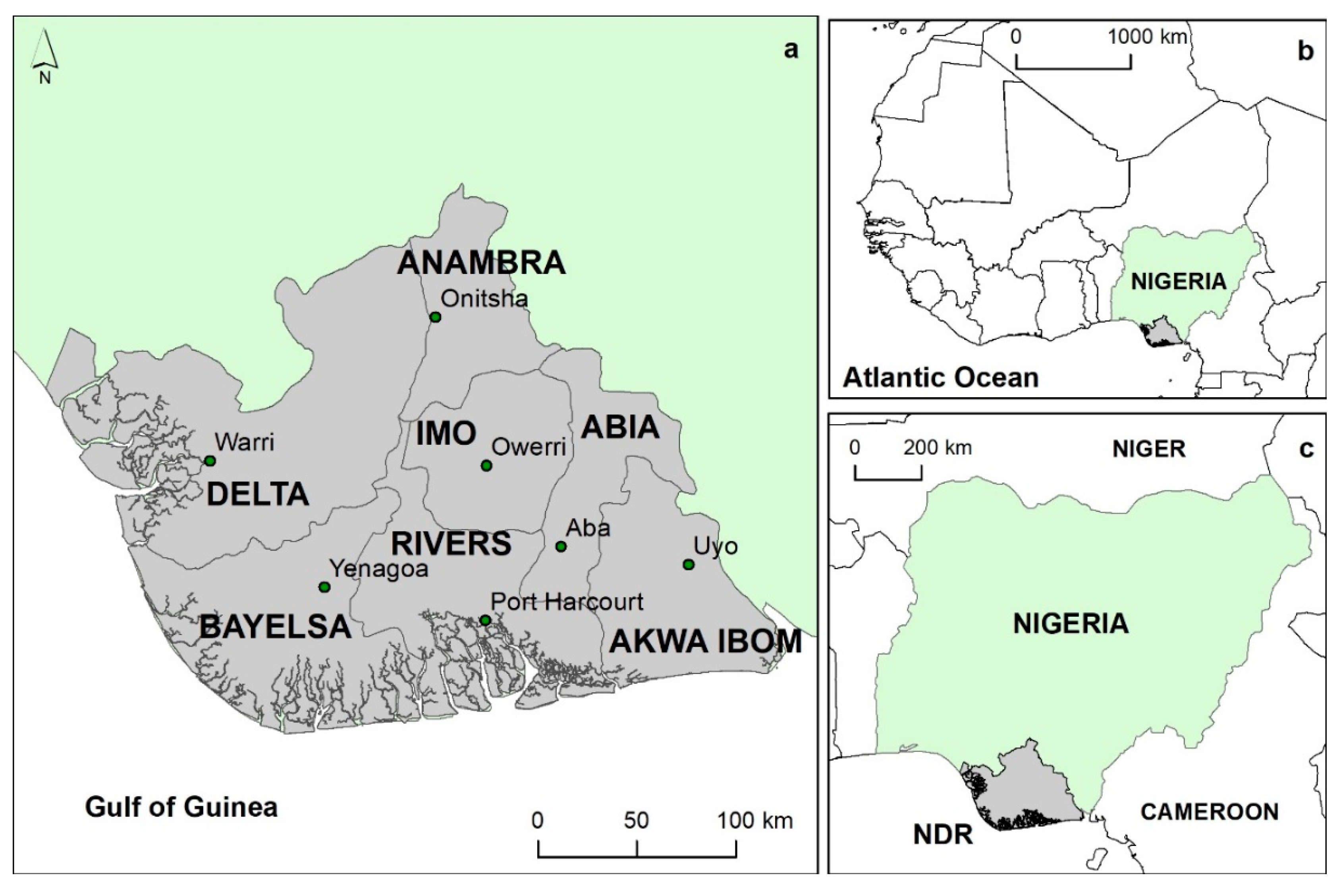
Figure 1. (a) Our delineation of the Niger Delta Region (comprising of the states of Abia, Akwa Ibom, Anambra, Bayelsa, Delta, Imo, and Rivers), and its location within (b) West Africa and (c) Nigeria.
Remotesensing 12 03619 g001
Figure 2. Methodological flowchart.
Remotesensing 12 03619 g002
Figure 3. Number of available observations from the Landsat USGS Level 1 archive for (a) the first epoch; (b) the middle epoch, and (c) the more recent epoch.
Remotesensing 12 03619 g003
Figure 4. Land cover over the Niger Delta Region in (a) 1988, (b) 2000, and (c) 2013. Pie charts show the respective estimates of the area covered by each land cover type (%); scale bar corresponds to (ac). Figures (d,e) are the losses and gains of each land cover type between 1988 and 2000; (f,g) the same for 2000–2013. The white background in (dg) signifies persistence.
Remotesensing 12 03619 g004
Figure 5. Intensity of the annual area of change within the two time intervals of the study. The dashed line is the uniform line (i.e., the output of Equation (2)).
Remotesensing 12 03619 g005
Figure 6. Category intensity analysis for the two periods. (a,c): gross annual area of gains and losses. (b,d): intensity of annual gains and losses within each land cover category. “# of elements” is the number of pixels. The dashed lines in (b,d) signify the uniform intensity value. Wa: Water; U: Urban; Wo: Woodland; B: Bareland; A: Agricultural: G: Grassland; DM: Degraded Mangrove; M: Mangrove.
Remotesensing 12 03619 g006
Figure 7. Landscape metrics for the mangrove and degraded mangrove classes. (a) Percentage of Landscape (%; PLAND); (b) Number of patches (NP); (c) Largest Patch Index (%; LPI); (d) Area weighted mean Euclidean nearest neighbour distance (m; ENN_AM); (e) Patch area median (ha; AREA_MD); (f) Area weighted Mean Patch Shape Index (SHAPE_AM); (g) Percentage of like adjacencies (%; PLADJ); (h) Euclidean nearest neighbour distance Standard Deviation (ENN_SD).
Remotesensing 12 03619 g007
Figure 8. Oil wells, pipelines, oil spills, and mangrove degradation hotspots in three parts of the study area: (a) the eastern area, around the city of Port-Harcourt; (b) the central area, near the river Bayelsa, and (c) the western area around the cities of Wari South and Wari South West. U: Urban; M: Mangrove; DM: Degraded Mangrove. (Oil spill data: https://www.nosdra.gov.ng and https://oilspillmonitor.ng. Oil wells and pipeline data: https://www.shell.com.ng).
Remotesensing 12 03619 g008
Table 1. Selection of landscape metrics used in this study with a short description of their relationship with mangrove forest fragmentation.
NameAbbreviationDescription
Percentage of Landscape (%)PLANDClass percentage in landscape (proportional abundance)
Patch area median (ha)AREA_MDThe median of patch areas in a class (a summary metric for the size of patches in the class, which is not influenced by very large patches)
Number of patchesNPThe number of patches in each class (simple measure of fragmentation)
Area weighted Mean Patch Shape IndexSHAPE_AMPatch shape complexity at class level (indicative of changes at the edges)
Largest Patch Index (%)LPIPercentage of total landscape area occupied by the largest-sized patch (measure of dominance)
Percentage of like adjacencies (%)PLADJThe proportions of like adjacencies to the total number of adjacencies for the class’ cells (aggregation)
Area weighted mean Euclidean nearest neighbour distance (m)ENN_AMEuclidean distance measured form patch edge to the closest patch edge from the same class (measures patch dispersion). Here we use the area weighted mean for the class to balance the influence of large patches.
Euclidean nearest neighbour distance Standard DeviationENN_SDMeasure of variation of ENN in the class (in comparison with the mean shows the form of distribution of patches in the class)
Table 2. Overall and per-class accuracy statistics for the three epochs (Wa: Water; U: Urban; Wo: Woodland; B: Bareland; A: Agricultural; G: Grassland; DM: Degraded Mangrove; M: Mangrove; CI: Confidence Interval; C = Correct; PA: Producer’s Accuracy; UA = User’s Accuracy).
1988 Landsat2000 Landsat2000
Landsat + JERS-1
2013 Landsat2013
Landsat + PALSAR-2
Overall
Accuracy
79.4882.3682.6181.2782.09
95% CI±0.003±0.0029±0.003±0.0027±0.0026
CPAUACPAUACPAUACPAUACPAUA
Wa737973758575758375748574788778
U709270819281819681849284889288
Wo847984878387878387848584848584
B617761498449488048508550508650
A818081888188888190887988877987
G716571536553546454566556576457
DM778277788678798579868286878287
M919091909090919091909290909390
Table 3. Contingency matrix for the two periods of study representing stable (in bold) and changed areas in km2. (a) 1988–2000; (b) 2000–2013. Wa: Water; U: Urban; Wo: Woodland; B: Bareland; A: Agricultural: G: Grassland; DM: Degraded Mangrove; M: Mangrove.
a 2000 (km2)
WaUWoBAGDMM1988 totalGross loss
1988Wa395.709.343.5912.937.720.6351.6620.58502.16106.46
U4.301444.7195.364.59341.9885.326.097.561989.91545.20
Wo11.61310.44193,54.713.601655.902020.5449.81363.9023,770.524415.81
B10.1010.090.3072.6719.140.190.120.28112.9040.23
A20.52543.09647.1539.388868.251439.747.485.8911,571.482703.24
G0.55572.512419.610.872883.363534.561.628.349421.415886.86
DM149.478.1713.410.353.451.641169.07454.691800.27631.20
M40.9026.06536.280.648.096.00535.475743.706897.151153.45
2000
Total
633.152924.41230,70.43135.0313,787.887088.631821.336604.94
Gross Gain237.461479.703715.7162.364919.643554.07652.25861.24
b 2013 (km2)2000 TotalGross Loss
2000Wa522.592.094.9110.264.160.4876.7713.16634.42111.83
U19.642150.29173.3818.35357.87184.3610.7210.192924.80774.51
Wo10.12371.4318,959.2221.031251.562038.8567.20351.52230,70.924111.70
B58.005.091.9957.1312.330.380.090.09135.1077.97
A25.86933.43939.5946.289083.422754.413.551.5813,788.124704.71
G1.34253.811784.195.441922.063113.855.572.387088.643974.79
DM157.763.6426.835.214.522.071158.61462.791821.42662.81
M65.307.86377.7714.217.687.84595.845529.726606.221076.50
2013
Total
860.613727.6322267.88177.9112,643.68102.241918.346371.43
Gross Gain338.021577.343308.66120.783560.184988.39759.74841.71
Table 4. Transition level intensity analysis FROM-Mangrove TO-all other classes (1988–2000 and 2000–2013). In bold and underlined: targeted classes (compared to uniform). Deg.: Degraded.
Transitions FROMMangrove
Time Interval1988–20002000–2013
TO CategoryObserved Annual Transition
(km2)
Transition Intensity
% of 2000 Category
Observed Annual Transition
(km2)
Transition Intensity
% of 2013 Category
Water2060.033320.05
Urban7170.035400.02
Woodland5060.0014310.01
Bareland400.042210.20
Agricultural4850.002980.00
Grassland2440.004610.01
Deg. Mangrove23,7991.5732,7421.80
Publisher’s Note: MDPI stays neutral with regard to jurisdictional claims in published maps and institutional affiliations.