Article

Flash Flood Susceptibility Modeling Using New Approaches of Hybrid and Ensemble Tree-Based Machine Learning Algorithms

by
Shahab S. Band
1,2,
Saeid Janizadeh
3,
Subodh Chandra Pal
4,
Asish Saha
4,
Rabin Chakrabortty
4,
Assefa M. Melesse
5 and
Amirhosein Mosavi
6,7,8,9,*
1
Institute of Research and Development, Duy Tan University, Da Nang 550000, Vietnam
2
Future Technology Research Center, National Yunlin University of Science and Technology, Douliou, Yunlin 64002, Taiwan
3
Department of Watershed Management Engineering and Sciences, Faculty in Natural Resources and Marine Science, Tarbiat Modares University, Tehran 14115-111, Iran
4
Department of Geography, The University of Burdwan, West Bengal 713 104, India
5
Department of Earth and Environment, AHC-5-390, Florida International University, Miami, FL 33199, USA
6
Faculty of Civil Engineering, Technische Universität Dresden, 01069 Dresden, Germany
7
School of Economics and Business, Norwegian University of Life Sciences, 1430 Ås, Norway
8
Kando Kalman Faculty of Electrical Engineering, Obuda University, 1034 Budapest, Hungary
9
Thuringian Institute of Sustainability and Climate Protection, 07743 Jena, Germany
*
Author to whom correspondence should be addressed.
Remote Sens. 2020, 12(21), 3568; https://doi.org/10.3390/rs12213568
Submission received: 7 September 2020 / Revised: 23 October 2020 / Accepted: 28 October 2020 / Published: 31 October 2020

Abstract

:
Flash flooding is considered one of the most dynamic natural disasters for which measures need to be taken to minimize economic damages, adverse effects, and consequences by mapping flood susceptibility. Identifying areas prone to flash flooding is a crucial step in flash flood hazard management. In the present study, the Kalvan watershed in Markazi Province, Iran, was chosen to evaluate the flash flood susceptibility modeling. Thus, to detect flash flood-prone zones in this study area, five machine learning (ML) algorithms were tested. These included boosted regression tree (BRT), random forest (RF), parallel random forest (PRF), regularized random forest (RRF), and extremely randomized trees (ERT). Fifteen climatic and geo-environmental variables were used as inputs of the flash flood susceptibility models. The results showed that ERT was the most optimal model with an area under curve (AUC) value of 0.82. The rest of the models’ AUC values, i.e., RRF, PRF, RF, and BRT, were 0.80, 0.79, 0.78, and 0.75, respectively. In the ERT model, the areal coverage for very high to moderate flash flood susceptible area was 582.56 km2 (28.33%), and the rest of the portion was associated with very low to low susceptibility zones. It is concluded that topographical and hydrological parameters, e.g., altitude, slope, rainfall, and the river’s distance, were the most effective parameters. The results of this study will play a vital role in the planning and implementation of flood mitigation strategies in the region.

1. Introduction

Floods are among the most destructive natural disasters [1]. The term flash flood can be defined as a phenomenon in which river water flows from its natural levees and causes inundation of the surrounding areas for a specific time [2]. It can be noted that flash floods are an unfavorable combination of different environmental parameters, i.e., meteorological, hydrological, geomorphological, and human intervention in the collapse of flash flood protection structures [3]. Over the last few decades, ongoing global climate change has been associated with an increase in the frequency and magnitude of global flash flood hazards. This is not the only reason why large-scale human intervention in the environment, such as forest ecosystems, e.g., deforestation, sedimentation in riverbeds, and riverbeds’ encroachment by human settlements and dam construction along with unhealthy development of urbanization, are responsible for devastating flash floods. In recent times, the flash flood intensity pattern has changed due to a gradual increase in the global population, especially in developing countries [4,5,6]. Flash flooding can cause significant socio-economic damages, i.e., loss of human settlement, fatality, infrastructural damages, i.e., agricultural land, buildings, communications, i.e., roads, railways [7,8,9]. Therefore, it has been estimated that 31% of total global economic losses with $104 billion are caused by flood hazards, known as the most costly natural disaster, among others [10]. In 2010, the World Statistics Survey also revealed that more than 178 million people were largely affected by devastating flash floods [11]. Flash flooding is also responsible for approximately 20,000 deaths every year, with 75 million people becoming homeless [12]. Iran is among the countries most susceptible to the flash flood. The Kalvan watershed has been affected by flooding annually; studies show that the Kalvan watershed is vulnerable to flash floods.
Multiple factors are responsible for the occurrence of a destructive flash flood, such as high intensity of rainfall, the tendency to generate runoff, rate of the rainfall-runoff process, soil properties and infiltration rate, poorly maintained flow pattern of a river system, and land-use changes. The frequency of flash floods is an essential method of analyzing flood hazards by predicting future flash floods. Therefore, flash flood frequency is measured using different historical flash flood data, i.e., discharge, rainfall, runoff [13]. As a result of devastating flash flood damage, various types of structural and non-structural measures should be taken to mitigate and prevent flash floods in a sustainable manner. Flash flood is considered to be one of the most dynamic natural disasters. and measures need to be taken to minimize economic losses and adverse effects. One of such measures is mapping the susceptibility areas for flash floods [14]. Accurate flash flood modeling and flash flood susceptibility mapping (FSM) analysis is the main concern among scientists and governments around the globe [15]. Statistical regression and time series analysis has been used for flash flood modeling for large basin areas [16]. The Hydrologic Engineering Center’s river analysis system (HEC-RAS) model [17,18] and MIKE model [19] are also used to predict spatio-temporal floods. The recognition of flood potential zones and the identification of different susceptible areas, i.e., high, moderate, low, are therefore necessary conditions for the mitigation and management of devastating flood hazards. In the last few decades, remote sensing and geospatial technology have been intensively used in flash flood susceptibility studies. This geospatial technology has been used for flash flood inundation mapping, site identification for flash flood shelter [13], and flash flood hazard assessment of tropical rainy areas [20]. Later on, different statistical methods in combination with geospatial technology were used for flash flood susceptibility analysis. Among these, multi-criteria decision analysis (MCDA), analytical hierarchy process (AHP), evidential belief function (EVF), etc. are notable methods. In recent decades, different types of machine learning (ML) models have received more attention among researchers throughout the world to predict flash flood susceptibility because of their high accuracy and capacity to handle complex input data structures. Different types of machine learning (ML) algorithms such as logistic regression (LR), artificial neural network (ANN), support vector machine (SVM), random forest (RF), boosted regression trees (BRT), generalized linear model (GLM), etc., along with different ensemble approaches, have been used to predict flash flood susceptibility. Extensive literature review shows that various ML algorithms, together with novel ML ensemble methods, were used to map flash flood susceptibility [3,15,21,22,23].
In recent times, studies have shown that hybrid or combined models have been used to evaluate flash flood susceptibility mapping rather than using a single ML model [24,25]. Thus, hybrid models are generally developed by integrating several statistical or ML models [26]. On the other hand, the ensemble methods were used to achieve the best performance with high predictive accuracy and were primarily developed by boosting or bagging more than one ML algorithm [25]. Due to the problem of overfitting in previous models such as random forest (RF) and decision tree [27], in this study, we used hybrid parallel and regularized methods to reduce errors in the RF model. In addition, the ensemble decision tree model including extremely randomized trees (ERT) was used in predicting flood susceptibility. In summary, the core aims of this study are: (i) Comparing hybrid parallel random forest (PRF), regularized random forest (RRF), and ERT with RF and boosted regression tree (BRT) as a benchmark model, (ii) prepare flash flood susceptibility maps based on hybrid and ensemble models, (iii) identifying most important variables on flash flood susceptibility in the Kalvan watershed.

2. Materials and Methods

2.1. Description of the Study Area

The Kalvan watershed is in the northwestern part of Markazi Province, Iran. The study area is located at 34°20′ and 34°50′ N and at 48°54′ and 49°29′ E and covers approximately 2056.75 km2. Elevations change from 1602 to 2660 m above sea level (Figure 1). Based on the Meteorological Department of Markazi Province, the watershed receives an average annual rainfall of 299 mm. The climate is arid to semi-arid. The significant volume of precipitation in the watershed happens during January and February, and the highest recorded 24-h rainfall total was about 47 mm. The dominant land uses, or land covers (LU/LC) in the Kalvan region are agriculture, rangeland, orchard, bare land, rock land, and urban; agriculture accounts for the most considerable portion of the region (Figure 3h).

2.2. Methodology

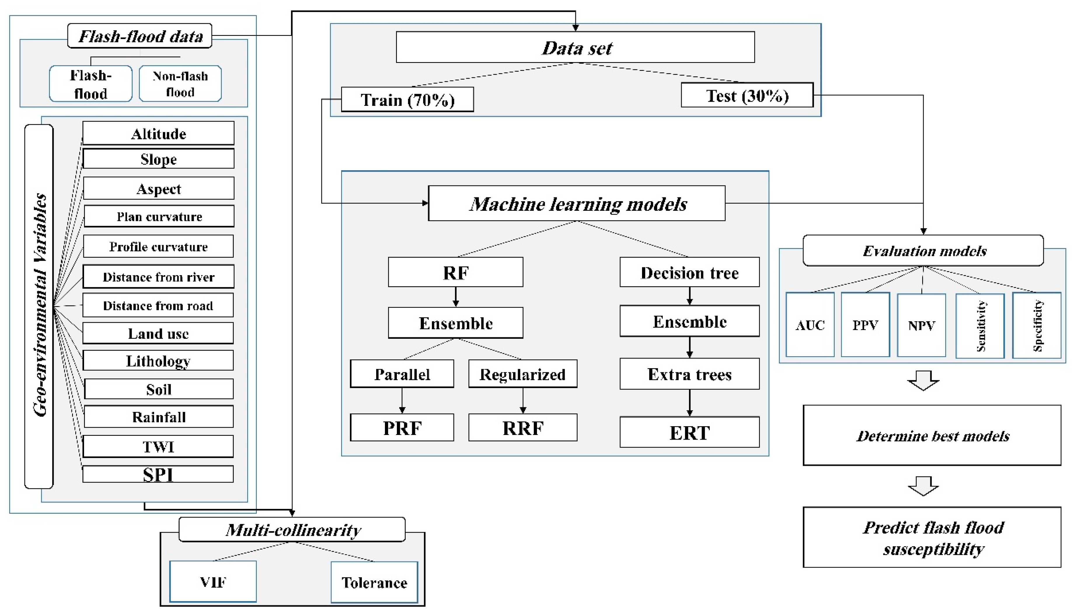
The methodology of the study is shown in the flowchart (Figure 2). The steps followed below summarize the approach used.
I.
A total of 256 flash flood susceptibility points were recognized based on field visits and information of the Department of Regional Water of Markazi Province.
II.
Thirteen flash flood susceptibility conditioning factors were chosen for modeling FSM.
III.
The multi-collinearity analysis was done among the flash flood susceptibility conditioning factors using the variance inflation factor (VIF) and tolerance (TOL) techniques.
IV.
Random forest model hybrid with two algorithmic regularizations and parallel for flash flood modeling was used.
V.
Extremely randomized trees such as an ensemble of a decision tree were used for flash flood modeling.
VI.
Flash flood susceptibility maps were prepared using BRT, RF, parallel and regularization methods on random forest and ensemble for extremely randomized trees (ERT).
VII.
Different flash flood susceptibility models’ performances were validated through statistical indices along with receiver operating characteristic (ROC)-AUC analysis.

2.3. Dataset Preparation for Spatial Modeling

In this study, flash flood susceptibility locations were provided based on flash flood events that occurred and were recorded by the Department of Regional Water of Markazi Province. A total of 256 flash flood points were used in this study. In order to determine the non-ditch points, geographic information system (GIS) software was used, and 256 points were randomly selected. The digital elevation model (DEM) map was obtained with a pixel size of 12.5 m from the ALOSPALSAR sensor, and the slope map, direction curve, plan curvature, profile curvature in the GIS software environment were prepared based on the DEM. The map of the distance from the waterway and the distance from the road based on the Euclidean extension was obtained in GIS software. A drainage density map was prepared using line density extension. System for Automated Geoscientific Analyses Geographic Information System (SAGA GIS) software was used to map the stream power index (SPI) and topographic wetness index (TWI). The region’s soil depth map was obtained based on the map prepared by the Administration of Natural Resources of Markazi Province. The lithological map was prepared based on the geological map of 1:100000 of the country’s mapping organization. Land use maps were prepared based on Landsat satellite images, Operational Land Image (OLI) measurement, and using the maximum likelihood algorithm with a Kappa value of 0.87 in the environment for visualizing images (ENVI) software environment. The precipitation map of the area was prepared from the rainfall records of six climatological monitoring stations for the period of 28 years and based on the inverse distance weighting (IDW) interpolation method.
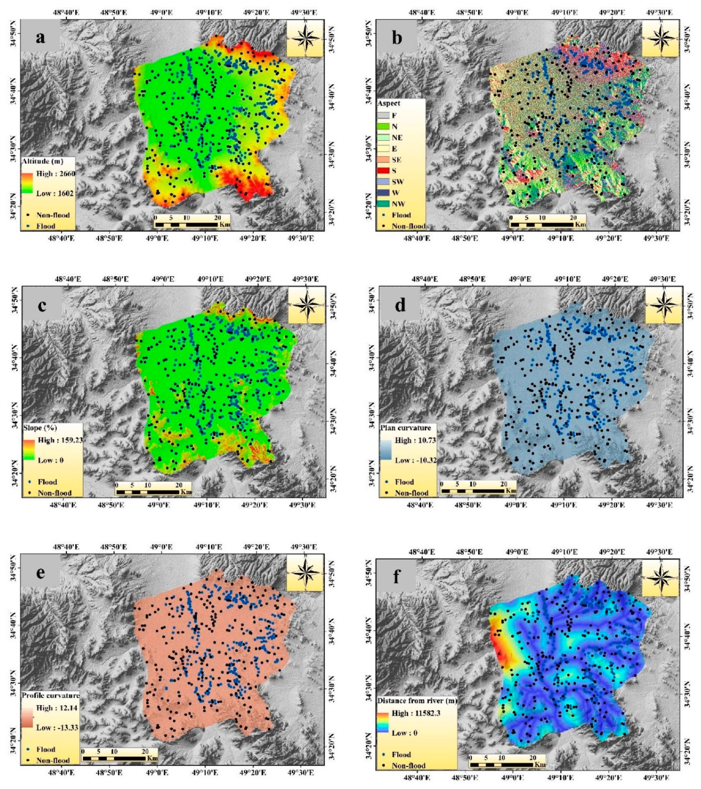
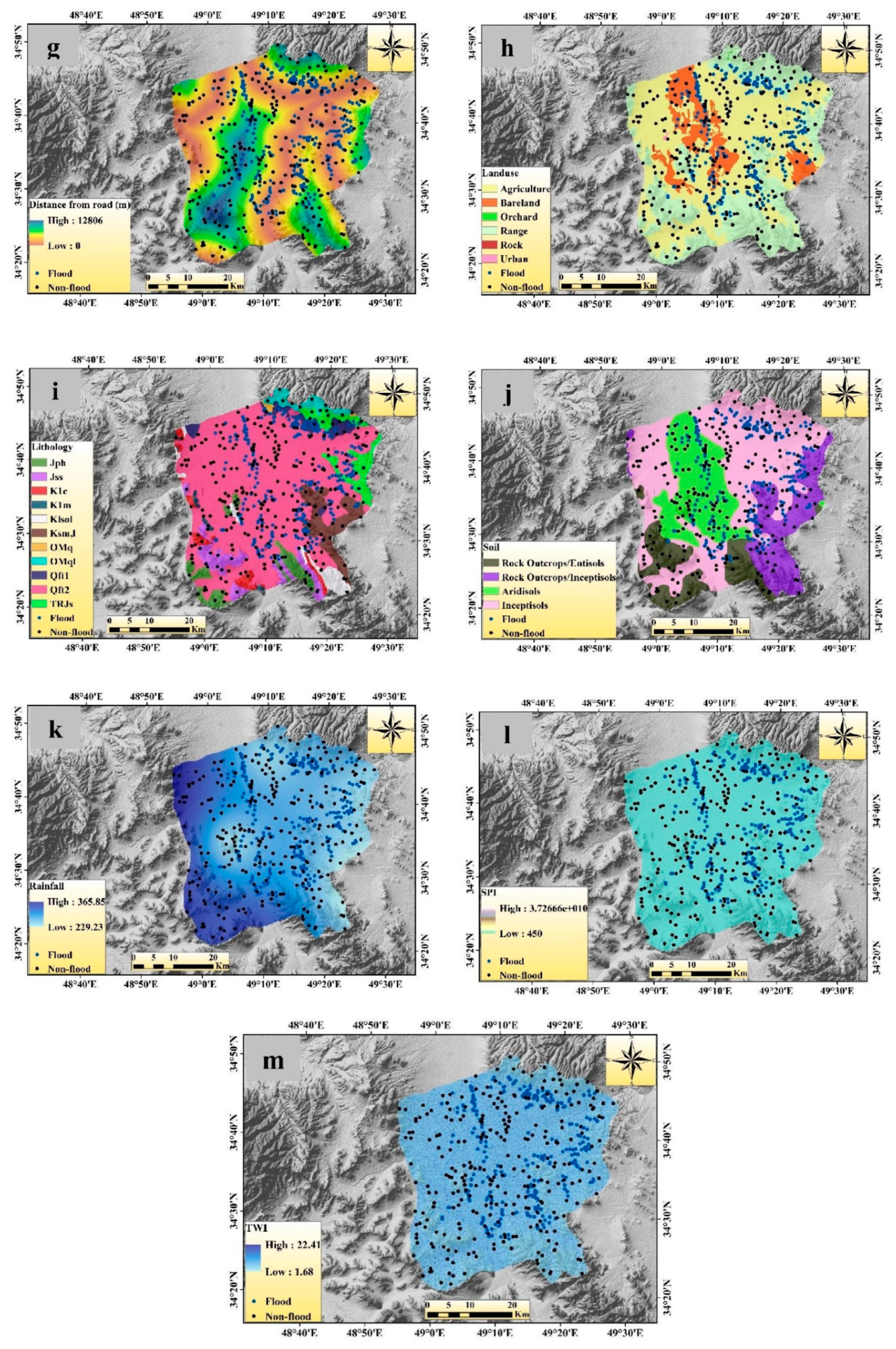
In this study, 13 geo-environmental variables that directly affect the flood process were chosen for the model setup and analysis. These variables or factors were altitude, slope, aspect, plan curvature, profile curvature, distance from river, distance from road, land use, lithology, soil depth, rainfall, stream power index (SPI), and topographic wetness index (TWI) (Figure 3a–m). Altitude was an important factor in the conditioning of flash floods, since it affects the natural flow of water. Generally, higher altitude areas are essentially safe from flash flooding (Das et al. 2019) and lower altitude areas have high potential for inundation during the flash flood times. The range of altitude varied from 1602 to 1660 m (Figure 3a) in this study area. The aspect indicated the direction of the slope and the flow pattern depended largely on the direction of the surface. Here, the slope aspect map was classified into nine classes (Figure 3b). Slope was also an important factor for the FSM, as it has a major influence on the runoff pattern and the flow of water. As a result, flash floods in the lower angle slope area are more frequent than in the higher angle slope area. The slope map is shown in Figure 3c and the percentage of slope ranges from 0 to 159.23. Topographic characteristics of an area were basically understood by plan and profile curvature. Here, the plan and profile curvature value ranged from −10.32 to 10.73 (Figure 3d) and −13.33 to 12.14 (Figure 3e).
The distance from the river was the most important factor in the flash flood susceptibility analysis. Flash flood frequency and magnitude were much high near the river and vice versa. Basically, the extension of flash flood and its magnitude largely depended on the distance from river [28]. The value of the distance from river map ranged from 0 to 11,582.3 m (Figure 3f). The distance from road network was also a critical flash flood conditioning factor. Roads are constructed based on a high-altitude area, so the pattern of water flow changes closer to the road as well, although high-intensity flash floods generally destroy the road structure. The distance from the road network map (Figure 3g) indicated that its value ranged from 0 to 12,806 m. The flash flood occurrence of an area largely depends on the land use/land cover (LULC) of that area. There was a negative correlation between the vegetation density and the occurrences of flash flood. Therefore, vegetation-prone areas had less runoff than the non-vegetation covered areas. The LULC map was prepared based on Landsat satellite images, OLI measurement, and the maximum probability algorithm in the ENVI software environment (Figure 3h). The present study was classified into six categories: i.e., agriculture, bare land, orchard, range, rock surface, and urban areas. Water percolation and its stagnation are largely dependent on the characteristics of the rocks. Therefore, lithology is an important parameter for the occurrence of flash floods in the area. The lithology of the present study area was classified into 12 classes (Figure 3i). The lithology map was provided based on the geological map of 1:100,000 of the Iranian National Cartographic Center (NCC). The significance of the soil type in the event of a flash flood is very high. Basically, the water storage capacity, percolation and permeability rate, and the drainage structure determined by soil types accelerate the area’s flash flooding [29]. The soil types map (Figure 3j) of the present study area was classified into four categories, namely rocky outcrops/Entisols, rocky outcrops/Inceptisols, Aridisols, and Inceptisols. The soil type map was obtained from the Administration of Natural Resources of Markazi Province. Rainfall is a direct factor in the occurrence of flash floods and the intensity of rainfall is a major factor in the magnitude of the flash floods. The amount of rainfall varies from 229.23 to 365.85 mm (Figure 3k). The precipitation map of the Kalvan watershed was prepared from the data of 6 climatological stations around the case study with a statistical period of 28 years (1991–2019) based on the IDW method.
The SPI can be defined as the power of erosion and degree of water discharge of a particular area within a watershed. It is established that if the SPI value is high, the flash flood power will also be high, and vice versa [2]. The SPI values have been calculated by using the following equation [30]:
S P I = A i t a n β  
where A i indicates a particular river basin area and t a n β indicates the slope gradient in degree. The SPI map of the present study area is shown in Figure 3l. TWI basically represents the moisture condition of the soil, water depth, and saturation zone of a specific topography [31]. TWI is widely used to know hydrological processes over topographical controls of a particular area. High TWI values represent more flash flood-prone areas than low TWI values. The following equation has been used to calculate TWI [32]:
T W I = K n ( A i t a n β )
where A i indicates a particular river basin area and t a n β indicates the slope gradient in degree. SPI and TWI variables were prepared in SAGAGIS 2.6 software.

2.4. Multi-Collinearity Analysis

Different geo-environmental factors have been used to predict flash flood susceptibility mapping using various kinds of models. It is necessary among all of these conditioning factors to find out which two or more than two factors are highly correlated with each other. If there is a higher correlation between two or more conditioning factors than the model, it is less valid to evaluate and to automatically reduce the accuracy of the output result. Therefore, multi-collinearity analysis helps to identify these highly correlated factors. Basically, multi-collinearity is a statistical analysis among more than two variables and represents a linear dependency between these variables [33]. Thus, high multi-collinearity conditioning factors need to be removed from the models for better prediction of the result [34]. Generally, variance inflation factor (VIF) and tolerance (TOL) techniques have been used to analyze the multi-collinearity. Different literature studies have shown high multi-collinearity found among all of these factors which have VIF values >5 or 10 and TOL values of <0.10 or 0.20 [35,36]. The TOL and VIF of a multi-collinearity analysis can be calculating using the following equation:
T O L = 1 R j 2
V I F = 1 T O L
where R j 2 represents the regression value of j on other different variables in a dataset.

2.5. Machine Learning Method Used in Flash Flood Susceptibility Modeling

2.5.1. Boosted Regression Tree (BRT)

BRT is a combination of statistical (egression trees) and machine learning (gradient boosting trees) techniques. Thus, BRT is also known as stochastic gradient boosting. BRT is an important data mining technique of a nonparametric method used to measure the association between dependent and independent variables [37]. It is very much used for the determination of independent variables and classification and forecasting analysis [38]. Among the two techniques used in BRT, boosting is used to improve model accuracy through appropriate new trees for residual error [39]. In addition to boosting, regression trees are used in BRT model to categorize the classification system from the decision tree groups in the model [40]. Generally, three parameters are needed for the optimization of a BRT model and these are a number of boosting tree iterations, interaction tree depth, and shrinkage [41]. The shrinkage is emphasized by the contribution of trees to the cultivated model. The parameter of the interaction tree depth is determined through the individual trees [42]. The function of BRT is basically based on the predictive variables X = { x 1 , x n } and a response variable y . The BRT model can be processed by using the training sample of { y i , X i } , i = 1 , N of known y and X values. We also wish to find out a function, i.e., F * ( X ) , which generally maps X to y. Thus, Equation (5) is used to minimize the values of a loss function among all the values of (y, X) [43]:
F * ( X ) = ψ ( y ,   F ( X ) )
The following equation is used for gradient boosting approximates F ( X ) :
F ( X ) = m = 0 M F m ( X ) = m = 0 M β m g ( X ; α m )  
where g ( X ; α m ) indicates a regression tree of a particular node, α m indicates the parameters of the tree, i.e., different splitting variables and split points, and β m indicates coefficients.
Finally, the BRT model is described by following equation given by Friedman in 2001 [43]:
F ( X ; [ β m α m ] m 0 ) = m = 0 m β m h ( X ; a m )  
where h ( X ; a m ) indicates the classification function with α parameters and X variables, m represents the variable of the stage of the model, and β m indicates the coefficient in the stage of m.

2.5.2. Random Forest (RF)

The algorithm of RF was developed by Breiman in the year 2001 [44]. It is an ensemble classifiers system based on binary decision trees. It can easily handle a large number of variables and it is basically a statistically-based approach [45]. By using the training dataset in the RF model, it generates numerous trees based on random bootstrapping, i.e., a random subset of the original training data [44]. The random bootstrapped sample also allows data not included, i.e., the remaining fallow subset data known as out of the bag (OOB) data [46]. This OOB data is used to assess the general errors in the model. The RF model is also used to analyze the dynamic trends known to non-linear interactions between explanatory and response variables. Besides this, any kind of assumption does not need to establish the relationship among explanatory and response variables in this model. Therefore, the RF algorithm has been used to analyze hierarchical and non-linear interactions in the big dataset along with better prediction of new-fangled data cases [47]. The RF requires three parameters to be tuned, i.e., number of variables (mtry), number of trees (ntree), and utmost number of terminal nodes (nodesize) [48]. The algorithm of RF is based on tree-structured classifiers and has been shown as follows:
h ( x , i k ) , k = 1 , 2 , n  
where i k represents flash flood occurrence conditioning factors; and 1, 2,…n are input vector x.
In an RF, the general errors can be defined as follows by Masetic and Subasi [49]:
G E = P x , y ( m g ( x , y ) < 0 )  
where x and y indicate the different flash flood occurrence conditioning factors, and mg represents the margin function. Again, the margin function can be described as follows:
m g ( x , y ) = a v k I ( h k ( x ) = y ) m a x j i a v k I ( h k ( x ) = j )  

2.5.3. Parallel Random Forest (PRF)

Traditional RF algorithms are not suitable for the analysis of big dataset. Therefore, the traditional RF algorithms for the analysis of large mass dataset parallelized design have been developed and are popularly known as PRF. The RF is generally an ensemble of different classification and regression tree (CART) decision trees and the implementation of parallel in traditional RF is better to analyze big datasets [50]. The RF model may be developed in parallel due to the ensemble of decision trees in the RF model. Basically, PRF is a modern version of RF based on decision tree computation [51]. In the real-time situation, RF was parallelized to minimize the execution time and to produce RF predictive output faster than that of the previous one [52]. In the PRF analysis, at first RF was divided into a variety of sub-forests. After that, these sub-forests were created in parallel and finally, all these sub-forests joined together in a larger forest at the core of the process. In PRF, massive dataset analysis is done in two ways: The first is the map, i.e., it creates different key value pairs in which the key indicates the index of a specific data value, and the second is the reduce, i.e., the analysis of key value pairs generated by the map function and the output of the final result [50].
The training dataset in the PRF model has been divided into different subsets of features due to splitting. Let us consider that the training dataset size is represented in S which is N   x   M , then independents variables represent x 0 ,   x 1 , x m 2 and dependent variables are x m 1 in that dataset. Later on, the dataset may be split into an ( M 1 ) feature subset. After that, each and every subset of features is loaded into the different data node. Finally, each subgroup of features is handled by a map mission, and trees are created in parallel.

2.5.4. Regularized Random Forest (RRF)

The RRF was generally developed for feature selection with one ensemble method [53] rather than several ensemble methods [54]. In this model, every element of the training dataset was analyzed at every tree node. It is also known that the process of selecting the features of the RRF model is greedy. In the RF model, the tree regularization method used to develop RRF could choose the compression function subset of the model [55]. Basically, the RRF algorithm has been developed in the way of RF, but the major distinction is that in RRF, the regularized information gain, i.e., G a i n R ( X i , v ) , is used.
G a i n R ( X i , v ) = { λ × G a i n ( X i , v )     i F G a i n ( X i , v )        i F  
where F represents the set of features used for splitting the tree nodes, λ [0, 1] represents penalty coefficient, and i F represents the coefficient penalized for the ith feature of splitting node v . Here λ represents larger penalty.
In RRF, minimum regularization occurs when λ = 1 and it is referred to as RRF (1). In RRF (1), the selection of feature subset is known as the least regularized subset, which indicates minimum regularization from RRF.

2.5.5. Extremely Randomized Trees (ERT)

The ERT model, also known as extra trees (ET), is a set of techniques based on a tree-based decision-making model. This is a specific randomization method proposed by Geurts et al. [56]. This model develops a number of regression trees or decision trees from the overall dataset [57]. The main difference between the RF and the ERT is that the ERT emphasizes randomness during training [58]. Randomization in the tree diversity helps to minimize the correlation; it means decision trees become more independent. In the ERT model, each tree node is randomly divided by the variable index and the splitting value. The main fundamental principle in the ERT model is the use of different decision trees, which are basically individually fragile learners, but when they are combined they become extremely robust learners [59]. The ERT algorithm is constructed on the basis of three parameters, i.e., the number of set decision trees (M), the number of randomly selected features (K), and the number of instances required to split the node ( n m i n ). The training dataset in the ERT model, X = { X 1 , X 2 , , X N } in which, sample X i = { f 1 , f 2 , , f d } is a D-dimensional vector and f j represents the feature and j { 1 , 2 , D } , and finally ET creates M-independent decision trees for the model.
The ERT model gives more accuracy and a superior result than the RF because this model removes discretization threshold values through optimization [56]. This model also has an important advantage of minimum computing times and can be easily implemented.

2.6. Methods of Validation and Accuracy Assessment

The validation and accuracy assessment of FSM using the machine learning model is very much necessary to evaluate the predictive result. Therefore, in this study, different statistical indices along with area under receiver operating characteristic (AUROC) curves were used to evaluate the five machine learning output results. In statistical indices, sensitivity (SST), specificity (SPF), positive predictive values (PPV), and negative predictive values (NPV) were used. If the result of these statistical indices showed a higher value, then every machine learning model gave a better result and vice versa [60]. The four statistical indices which were used in this study can be calculated by following equations
S S T = T P T P + F N  
S P F = T N F P + T N  
P P V = T P F P + T P  
N P V = T N T N + F N  
where TP represents true positive, TN represents true negative, FP represents false positive, and FN represents false negative.
On the other hand, the standard tool widely used for model validation and accuracy assessment is ROC-AUC. The ROC curve plotted on the X and Y axis is popularly known as sensitivity and 1-specificity. This X and Y axes represent true positive and false positive in the graph and the optimum value in both cases is 1 [61]. The ROC-AUC range varies from 0.5 to 1, indicating poor performance to excellent model validation performance. The ROC-AUC has been computed by using following equation:
S A U C = k = 1 n ( X k + 1 X k ) ( S k + 1 S k + 1 S k 2 )  
where S A U C is the area under curve, X k is the 1-specificity, and S k is the sensitivity of the receiver operating characteristic (ROC) curve.

3. Results

3.1. Multi-Collinearity Analysis

For this analysis, the multi-collinearity test of 13 flash flood causative factors was done considering the VIF and TOL limit (Table 1). The range of VIF was about 1.07 to 2.44, and the highest and lowest values of VIF were associated with slope and aspect. In the case of TOL, the range was about 0.41 to 0.93. The highest and lowest values of the TOL limit were associated with aspect (0.93) and slope (0.41). There was no such problem of multi-collinearity in the selected variables for estimating the flash flood susceptibility. Therefore, all 13 explanatory variables were used for modeling the flash flood susceptibility in the present study area.

3.2. Flash Flood Susceptibility Modeling

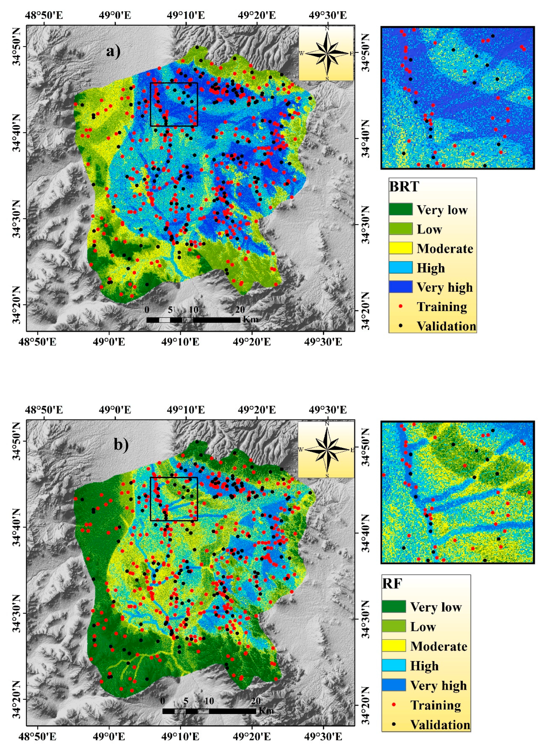
In the BRT model, the areal coverage of very high to high flash flood susceptible areas was 425.13 and 683.91 km2, respectively, and these zones were mainly located in the middle portion of the watershed (Table 2). The rest of the portion of this watershed was associated with moderate, low, and very low susceptible zones, and the areal coverage of these zones was 442.73 (21.53%), 404.28 (19.66%), and 100.70 km2 (4.90%), respectively (Figure 4a).
In the RF model, the very high, high, and moderate flash flood susceptibility zones were associated mainly in the northern, eastern, and middle portions of the watershed, and the areal coverage of these zones was 225.12 (10.95%), 384.4 (18.69%), and 440.21 km2 (21.40%), respectively. The rest of the part of this watershed was associated with low and very low flash flood susceptible areas and the areal coverage of these regions were 388.53 (18.89%) and 618.49 km2 (30.07%), respectively (Figure 4b).
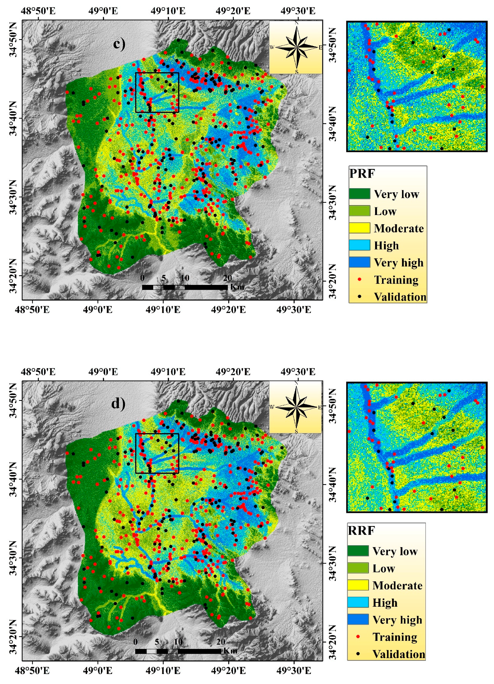
In the PRF model, the areal coverage of very high, high, and moderate flash flood susceptible areas was 239.72 (11.66%), 396.72 (19.29%), and 461.12 km2 (22.42%), and these susceptible zones were located mainly in the eastern, middle, and northern portions of the watershed. Apart from this, the rest of this region was associated with low to very low flash flood susceptible zones, and the areal extent of these zones was 440.96 (21.44%) and 518.23 km2 (25.20%), respectively (Figure 4c).
In the case of the RRF model, the areal coverage of very high, high, and moderate flash flood susceptible areas was 247.98 (12.06%), 373.75 (18.17%), and 466.56 km2 (22.68%), and these susceptible zones were located mainly in the eastern, middle, and northern portions of the watershed. Apart from this, the rest of this region was associated with low to very low flash flood susceptible zones, and the areal extent of these zones was 359.57 (17.48%) and 608.89 (29.60%), respectively (Figure 4d).
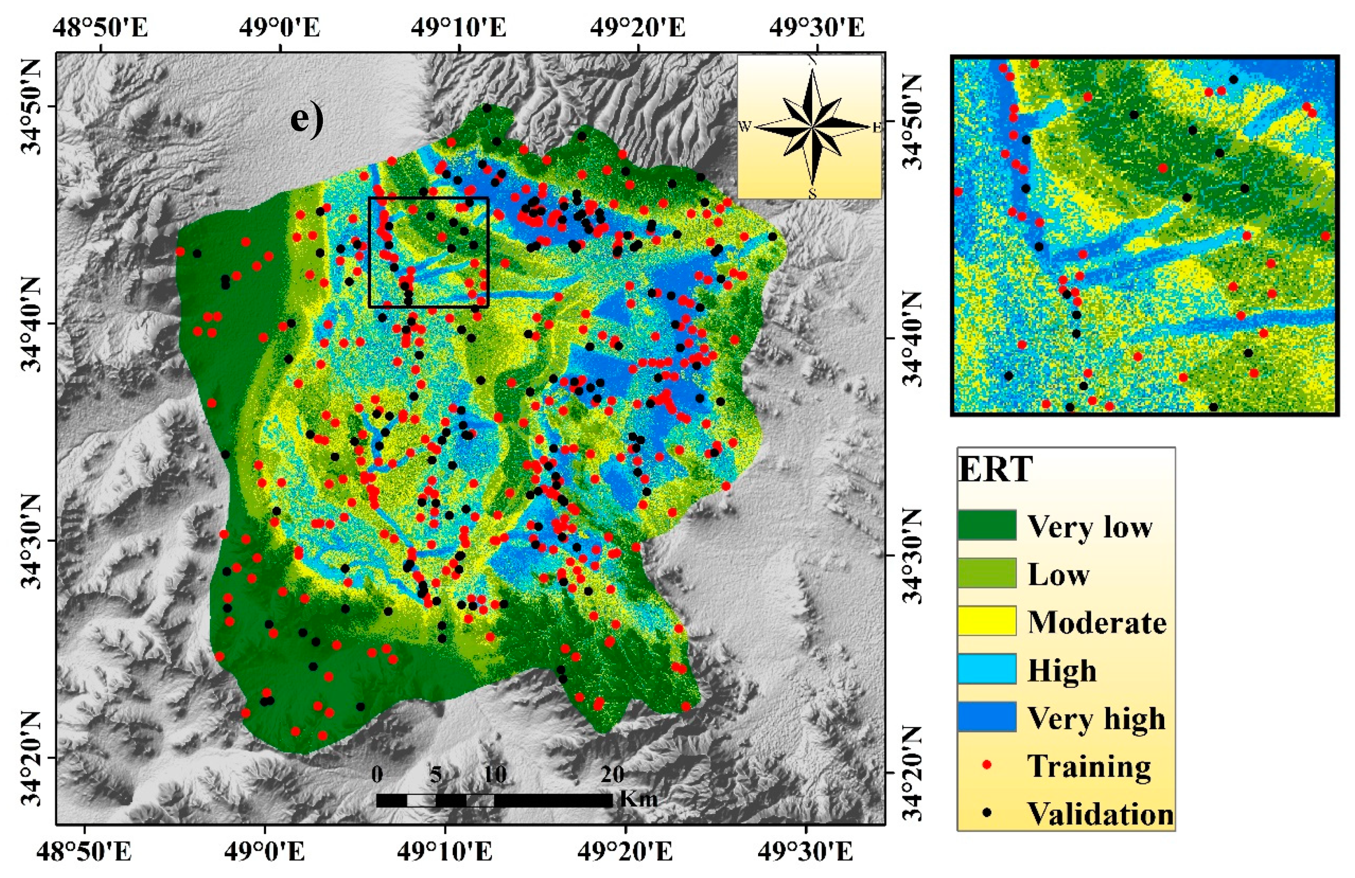
In the ERT model, the very high, high, and moderate flash flood susceptibility zones were associated mainly in the northern, eastern, and middle portions of the watershed, and the areal coverage of these zones was 249.84 (12.15%), 332.72 (16.18%), and 391.51 km2 (19.04%), respectively. The rest of the part of this watershed was associated with low and very low flash flood susceptible areas, and the areal coverage of these regions was 431.14 (20.96%) and 651.54 km2 (31.68%), respectively (Figure 4e).

3.3. Evaluation of Parameters

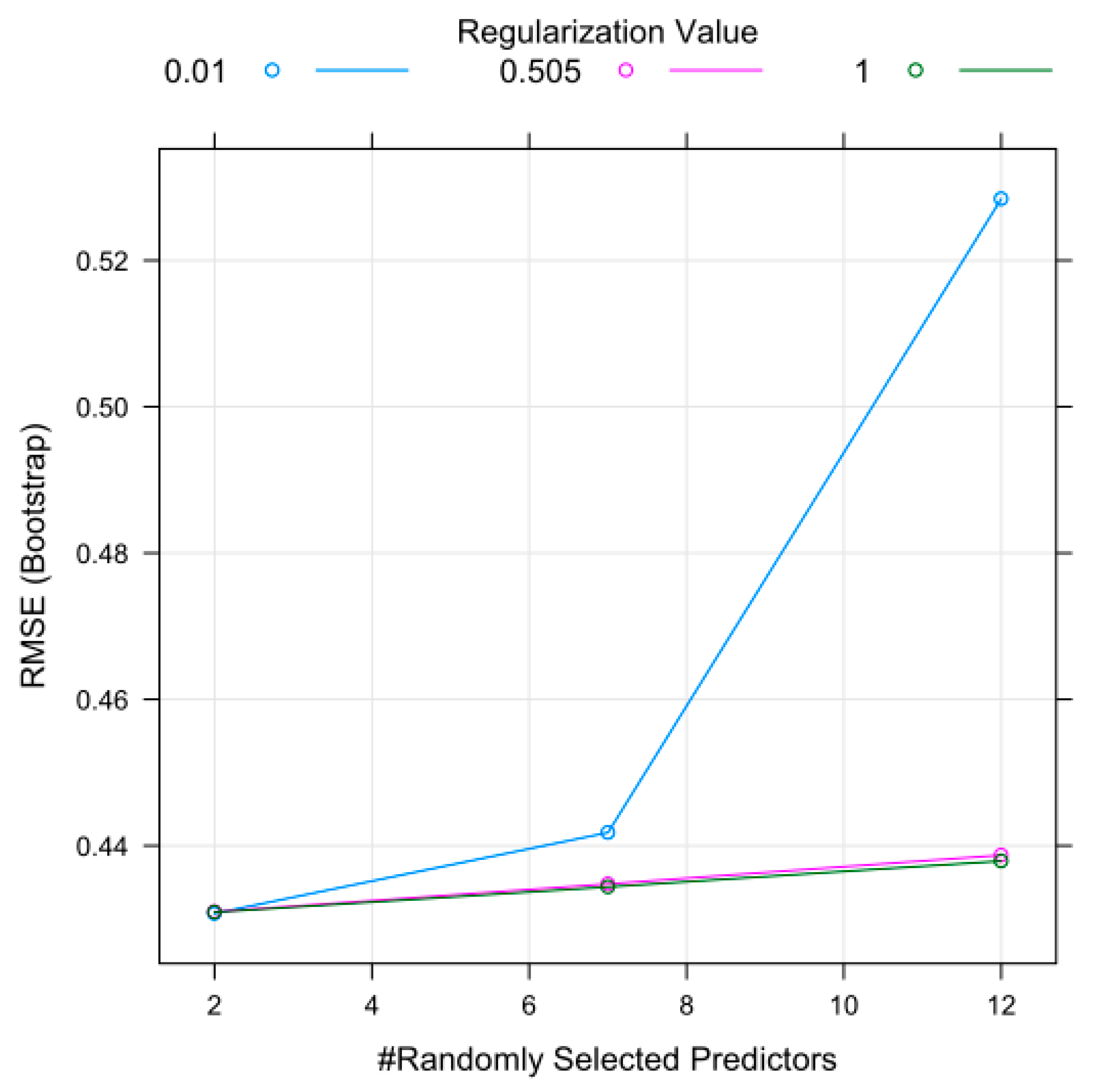
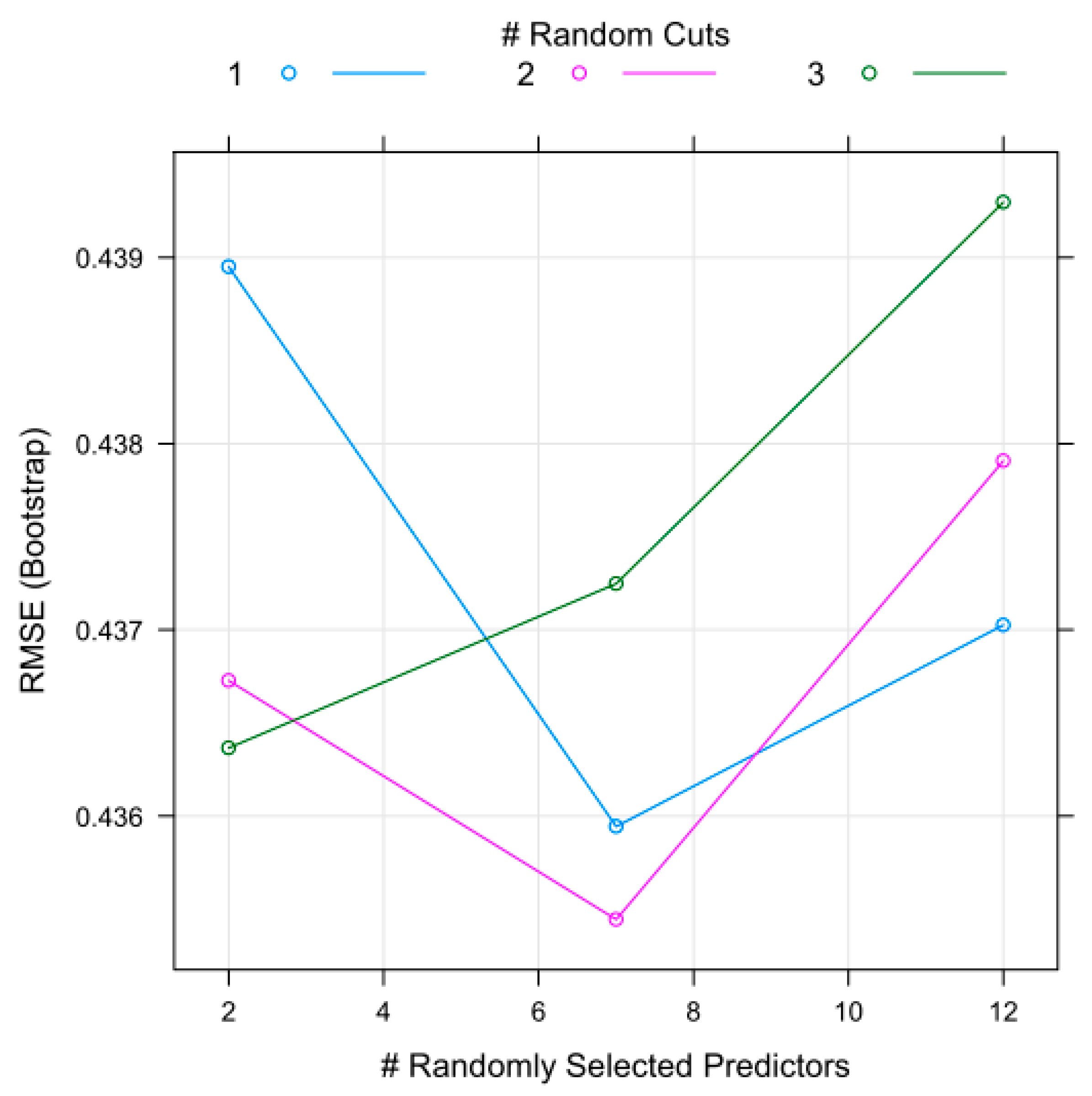
The results of parameter evaluation versus error rate (RMSE) in the two RRF and ERT models are shown in Figure 5 and Figure 6. Based on Figure 5, it was found that in the RF model, the optimal amount of regularization was 0.01 and the mtry number 2 had the least error in flood modeling. In addition, the results of Figure 6 showed in the ERT model the optimal number of random cut 2 and the number of mtry 7 were determined with the least error in order to model the flood.

3.4. Validation of the Models

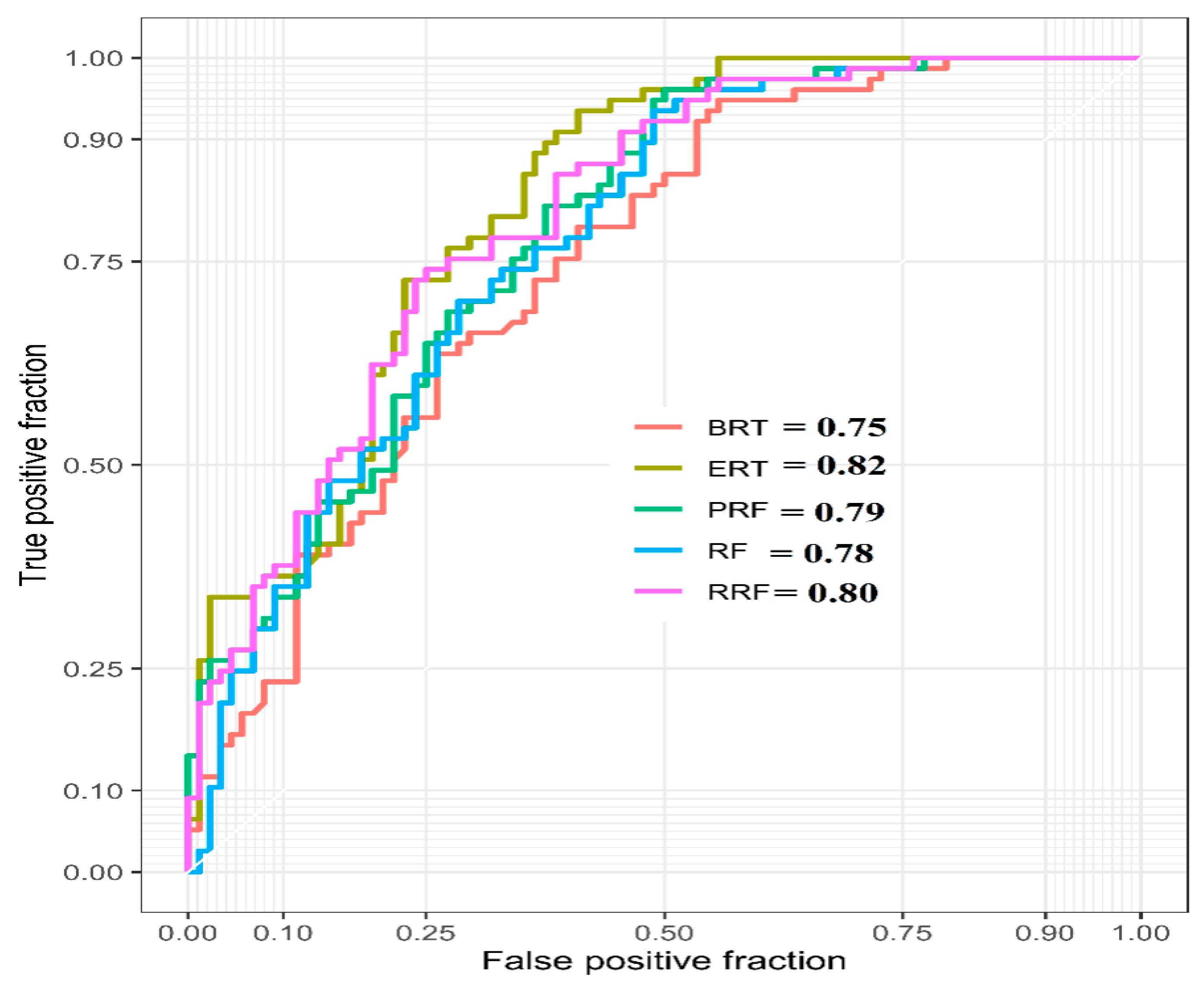
The validation of all the models was done with the help of the AUC values from ROC and different statistical indices. Considering the AUC, the best model was ERT and the AUC of this model was 0.82. Apart from this, the AUC values of the rest of the models, i.e., RRF, PRF, RF, and BRT, were 0.80, 0.79, 0.78, and 0.75, respectively (Figure 7). The AUC value for this perspective was estimated considering the true positive (TP) and false positive (FP) values of susceptibility modeling. The vertical axis and horizontal axis of this curve were representing the TP and FP values of susceptibility modeling. TPs were pixels which were correctly estimated to be susceptible to flash flooding and, otherwise, FPs were pixels which were incorrectly estimated to be susceptible to flash flooding. Seventy per cent of the overall data were considered to be model or training and the remaining thirty per cent was considered for validation purposes. The higher AUC values represented the higher accuracy, and vice versa. Here, all the models were associated with higher accuracy, but the ERT model was the most optimal for predicting the flash flood susceptibility. Apart from these, different statistical indices (i.e., sensitivity, specificity, PPV, and NPV) also indicated the same characteristics of all the predicted models (Table 3).

3.5. Importance Value

The importance of the variables of all the predicted models was estimated and is shown in Table 4. In the BRT model, the most important variables for predicting flash flood susceptibility were distance from river (100), rainfall (94.97), altitude (87.36), and slope (86.22). In the case of the RF model, the dominating variables for flash flood susceptibility were rainfall (100), altitude (81.89), and distance from river (75.03). In the PRF model, the most importance variables for flash flood susceptibility assessment were rainfall (100), altitude (79.53), and distance from river (74.81). In the RRF model, the dominating variables for predicting the flash flood susceptibility were rainfall (100) and distance from river (94.21), respectively. In the case of the ERT model, the most importance variables for generating the flash flood susceptibility model were distance from river (100), rainfall (94.97), altitude (87.36), and slope (86.22), respectively (Table 4). Other variables in all the predicted models were associated with moderate to lower importance for flash flood susceptibility assessment.

4. Discussion

In this study, various machine learning algorithms (i.e., BRT, RF, PRF, RRF, and ERT) were considered for estimating the flash flood susceptible areas with optimal accuracy. In most of the research work related to this field, the focus was on the use of various appropriate machine learning algorithms to estimate the effectiveness of susceptibility modeling. The application of machine learning and artificial intelligence techniques not only saved time and were less expensive, but were also associated with significant accuracy. For this reason, our main objective of this study was to identify the most efficient machine learning algorithm for estimating the flash flood susceptibility in a semi-arid environment. In this outcome, the ERT model (AUC = 0.82) was most optimal according to its predictive capacity, considering the values of AUC and different statistical indices, though there was a slight variation among the predicted models and its associated AUC values. This method created an ensemble of extremely randomized trees for the determination or estimation as per the traditional technique. Its primary differences from the other tree-based learning algorithms were that it divided clusters by randomly selecting cut-points, and it utilized the entire learning dataset to grow trees [56]. Forecasts of trees were also compiled to achieve the best estimation by most of the supports on supervised learning and mean estimation in the case of regression. From the perspective of bias-variance, a justification for the extra trees model was that the implied randomization of the cut-point and assign mixed with the ensemble average had to be able to minimize the deviation quite positively than lesser randomization strategies considered by different techniques. So far, many studies have proven the high ability of the ERT model in various fields of study. Zhou et al. [62] used extremely randomized trees for image classification for malware detection in comparison with KNN and RF, which showed the results were quite impressive with high accuracy rate. Eslami et al. [63] applied the ERT model to air quality forecasting and showed the high efficiency of the ERT model. Regarding the comparison of the ERT model with the random forest model, it should be noted that this model created a large number of trees and divided the nodes using random subset features the same as the random forest, but they had two main differences. In the ERT model, each tree node was randomly divided by the variable index and the splitting value. The ERT model’s main fundamental principle was the use of different decision trees, which were individually fragile learners, but when they were combined, they became extremely robust learners [59]. Although this method has been used in other fields of sciences, such as land cover classification [64] and modeling of daily lake surface water temperature [65], the effectiveness of this model in studying natural disasters, especially flash floods, has not been proven. The key aspect is using more sophisticated approaches like the ERT model to consider flash floods because the relationship between flood occurrence and its causes is not linear and requires very strong and complex models [66].
The importance of hydrological and topographical factors is more optimistic in flash flood susceptibility modeling. In the semi-arid environment, flash floods are one of the common natural hazards and have a serious impact on society. The hydrological factors like rainfall and river distance are the most influential elements in flash flood susceptibility. Apart from this, the topographical elements such as altitude and slope are the most important elements of susceptibility to flash flooding. There are different types of flash flood susceptibility research, which suggests the importance of topographic and hydrological elements as the most influential factors for flash flood susceptibility [18,60,67,68]. In the present study, the most important variables for predicting flash flood susceptibility are the distance from river, rainfall, altitude, and slope. One of the factors considered in flood vulnerability studies is the distance from the river. The areas near to river and stream are more sensitive to flooding and this is a fact that many studies have proved [26,69,70]. Our study showed a high correlation between areas close to the river and flood sensitivity, which was consistent with other studies. Rainfall is a main influencing factor in flood susceptibility mapping, which has been considerably observed in the other studies [71]. Among the topographic variables, slope has the greatest effect on the amount of surface runoff and, therefore, is known as the most critical influential variable in many flash flood studies [71,72,73]. Costache [74] showed that slope is the most crucial factor affecting the flash flood distribution in the Prahova river catchment, Romania. Altitude is one of the most important factors in flash flood modeling in this study area. According to the prepared flood susceptibility maps, it is clear that low-altitude areas, which are usually close to the riverbank, are affected by floods due to low slope and proximity to the river during floods. Various researchers have introduced the altitude factor as one of the factors affecting floods and have confirmed that low altitude areas are more sensitive to flooding [2,75,76].
Natural hazards such as flash floods have a severe impact on people and their livelihoods and the associated infrastructure [11,22]. This type of natural hazard cannot be prevented entirely, but its impact can be minimized by implementing appropriate strategies [77]. For this purpose, the modeling of flash flood susceptible areas with the incorporation of proper strategy is an essential part of monitoring and managing this hazard [78]. On the other hand, efficient modeling and mapping can minimize the severe impact of flash floods and reduce the chance of destroying people’s livelihoods, economy, and infrastructure [79]. Modeling flash floods’ susceptibility is one type of preparedness to reduce the impact of flash floods by implementing appropriate strategies [15]. However, the river basin level’s current outcome appears to help flash flood control officials once again. For this more comprehensive scale, including a river field, it is suggested that an integrated structural design be created that could more effectively consider the impact of anthropocentric variables to determine flash flood events for projected water discharge of varying probability. The main task of the future research is to develop the most suitable algorithm for creating such a type of hybrid models which could predict the scenario in a maximum optimal level after incorporating the lesser number of variables. The use of deep learning approaches due to their high accuracy is one of the solutions proposed for the future of natural hazard studies, especially flash floods studies.

5. Conclusions

This study was conducted to estimate the flash flood susceptibility of the Kalvan watershed in Iran. This region is generally associated with a semi-arid environment and very much prone to flash floods. Thus, the assessment of this type of hazard was necessary by incorporating a suitable algorithm for reducing the damages from it. For this purpose, we considered five hybrid parallel and regularized approaches to estimate the flash flood susceptibility in a more authentic way and with maximum possible accuracy. In this analysis, the most optimal model was ERT with an AUC value of 0.82. The rest of the models’ AUC values, i.e., RRF, PRF, RF, and BRT, were 0.80, 0.79, 0.78, and 0.75, respectively. In the ERT model, the areal coverage for a very high to moderate flash flood susceptible area is 582.56 km2 (28.33%), and the rest of the portion was associated with very low to low susceptible zones. Therefore, in order to avoid this kind of scenario, careful consideration and correct approaches need to be taken in this area. In the proposed susceptibility modeling, the importance of the topographical and hydrological parameters like altitude, slope, rainfall, and distance from the river were more effective than the other parameters considered in this study. Plan curvature, profile curvature, SPI, land use, etc. were associated with lower importance on flash flood susceptibility assessment. This outcome’s main novelty was the application and development of hybrid parallel and regularization approaches for estimating the flash flood susceptibility in a semi-arid environment. These models can be applied in any climatic condition and any type of susceptibility assessment. This type of outcome can help the regional planers and local administrators implement the development strategies for escaping this type of situation.

Author Contributions

S.J. acquired the data; S.J., S.S.B., A.M., and S.C.P. conceptualized and performed the analysis; S.C.P., A.S., R.C. and S.J. wrote the manuscript and discussion, and analyzed the data; A.M. supervised and completed the funding acquisition; A.M., S.S.B., S.J., S.C.P., A.S., R.C., A.M.M., and A.M. revised the manuscript. A.M. The validation had been jointly done by S.S.B., S.J., S.C.P., A.S., R.C., A.M.M., and A.M. Furthermore, S.J. provided technical sights, as well as edited, restructured, and professionally optimized the manuscript. All authors discussed the results and edited the manuscript. All authors have read and agreed to the published version of the manuscript.

Funding

This project was funded by the Hungarian State and the European Union under the EFOP-3.6.2-16-2017-00016 project.

Acknowledgments

Support of the Alexander von Humboldt Foundation is also acknowledged.

Conflicts of Interest

The authors declare no conflict of interest.

References

  1. Shen, G.; Hwang, S.N. Spatial—Temporal snapshots of global natural disaster impacts Revealed from EM-DAT for 1900–2015. Geomat. Nat. Hazards Risk 2019, 10, 912–934. [Google Scholar] [CrossRef] [Green Version]
  2. Chapi, K.; Singh, V.P.; Shirzadi, A.; Shahabi, H.; Bui, D.T.; Pham, B.T.; Khosravi, K. A novel hybrid artificial intelligence approach for flood susceptibility assessment. Environ. Model. Softw. 2017, 95, 229–245. [Google Scholar] [CrossRef]
  3. Roy, P.; Pal, S.C.; Chakrabortty, R.; Chowdhuri, I.; Malik, S.; Das, B. Threats of climate and land use change on future flood susceptibility. J. Clean. Prod. 2020, 272, 122757. [Google Scholar] [CrossRef]
  4. Khosravi, K.; Pourghasemi, H.R.; Chapi, K.; Bahri, M. Flash flood susceptibility analysis and its mapping using different bivariate models in Iran: A comparison between Shannon’s entropy, statistical index, and weighting factor models. Environ. Monit. Assess. 2016, 188, 656. [Google Scholar] [CrossRef] [PubMed]
  5. Yariyan, P.; Janizadeh, S.; Van Phong, T.; Nguyen, H.D.; Costache, R.; Van Le, H.; Pham, B.T.; Pradhan, B.; Tiefenbacher, J.P. Improvement of Best First Decision Trees Using Bagging and Dagging Ensembles for Flood Probability Mapping. Water Resour. Manag. 2020, 34, 3037–3053. [Google Scholar] [CrossRef]
  6. Janizadeh, S.; Avand, M.; Jaafari, A.; Phong, T.V.; Bayat, M.; Ahmadisharaf, E.; Prakash, I.; Pham, B.T.; Lee, S. Prediction Success of Machine Learning Methods for Flash Flood Susceptibility Mapping in the Tafresh Watershed, Iran. Sustainability 2019, 11, 5426. [Google Scholar] [CrossRef] [Green Version]
  7. Ferreira, S.; Hamilton, K.; Vincent, J.R. Nature, Socioeconomics and Adaptation to Natural Disasters: New Evidence from Floods; World Bank Group: Washington, DC, USA, 2011. [Google Scholar]
  8. Chowdary, V.M.; Chakraborthy, D.; Jeyaram, A.; Murthy, Y.V.N.K.; Sharma, J.R.; Dadhwal, V.K. Multi-criteria decision making approach for watershed prioritization using analytic hierarchy process technique and GIS. Water Resour. Manag. 2013, 27, 3555–3571. [Google Scholar] [CrossRef]
  9. Pham, B.T.; Avand, M.; Janizadeh, S.; Phong, T.V.; Al-Ansari, N.; Ho, L.S.; Das, S.; Le, H.V.; Amini, A.; Bozchaloei, S.K.; et al. GIS Based Hybrid Computational Approaches for Flash Flood Susceptibility Assessment. Water 2020, 12, 683. [Google Scholar] [CrossRef] [Green Version]
  10. Dano, U.L.; Balogun, A.-L.; Matori, A.-N.; Wan Yusouf, K.; Abubakar, I.R.; Said Mohamed, M.A.; Aina, Y.A.; Pradhan, B. Flood susceptibility mapping using GIS-based analytic network process: A case study of Perlis, Malaysia. Water 2019, 11, 615. [Google Scholar] [CrossRef] [Green Version]
  11. Khan, A.N. Analysis of flood causes and associated socio-economic damages in the Hindukush region. Nat. Hazards 2011, 59, 1239. [Google Scholar]
  12. Khosravi, K.; Nohani, E.; Maroufinia, E.; Pourghasemi, H.R. A GIS-based flood susceptibility assessment and its mapping in Iran: A comparison between frequency ratio and weights-of-evidence bivariate statistical models with multi-criteria decision-making technique. Nat. Hazards 2016, 83, 947–987. [Google Scholar] [CrossRef]
  13. Das, B.; Pal, S.C.; Malik, S. Assessment of flood hazard in a riverine tract between Damodar and Dwarkeswar River, Hugli District, West Bengal, India. Spat. Inf. Res. 2018, 26, 91–101. [Google Scholar] [CrossRef]
  14. Ali, S.A.; Khatun, R.; Ahmad, A.; Ahmad, S.N. Application of GIS-based analytic hierarchy process and frequency ratio model to flood vulnerable mapping and risk area estimation at Sundarban region, India. Model. Earth Syst. Environ. 2019, 5, 1083–1102. [Google Scholar] [CrossRef]
  15. Ali, S.A.; Parvin, F.; Pham, Q.B.; Vojtek, M.; Vojteková, J.; Costache, R.; Linh, N.T.T.; Nguyen, H.Q.; Ahmad, A.; Ghorbani, M.A. GIS-based comparative assessment of flood susceptibility mapping using hybrid multi-criteria decision-making approach, na{\″\i}ve Bayes tree, bivariate statistics and logistic regression: A case of Topl’a basin, Slovakia. Ecol. Indic. 2020, 117, 106620. [Google Scholar] [CrossRef]
  16. Bui, D.T.; Tsangaratos, P.; Ngo, P.-T.T.; Pham, T.D.; Pham, B.T. Flash flood susceptibility modeling using an optimized fuzzy rule based feature selection technique and tree based ensemble methods. Sci. Total Environ. 2019, 668, 1038–1054. [Google Scholar] [CrossRef] [PubMed]
  17. Brunner, G.W. HEC-RAS River Analysis System. Hydraulic Reference Manual. Version 1.0.; Hydrologic Engineering Center: Davis, CA, USA, 1995. [Google Scholar]
  18. Malik, S.; Pal, S.C. Application of 2D numerical simulation for rating curve development and inundation area mapping: A case study of monsoon dominated Dwarkeswar River. Int. J. River Basin Manag. 2020, 18, 1–11. [Google Scholar] [CrossRef]
  19. Zhou, Q.; Mikkelsen, P.S.; Halsnæs, K.; Arnbjerg-Nielsen, K. Framework for economic pluvial flood risk assessment considering climate change effects and adaptation benefits. J. Hydrol. 2012, 414, 539–549. [Google Scholar] [CrossRef]
  20. Biswajeet, P.; Mardiana, S. Flood hazrad assessment for cloud prone rainy areas in a typical tropical environment. Disaster Adv. 2009, 2, 7–15. [Google Scholar]
  21. Costache, R.; Bui, D.T. Identification of areas prone to flash-flood phenomena using multiple-criteria decision-making, bivariate statistics, machine learning and their ensembles. Sci. Total Environ. 2020, 712, 136492. [Google Scholar] [CrossRef]
  22. Chowdhuri, I.; Pal, S.C.; Chakrabortty, R. Flood susceptibility mapping by ensemble evidential belief function and binomial logistic regression model on river basin of eastern India. Adv. Sp. Res. 2020, 65, 1466–1489. [Google Scholar] [CrossRef]
  23. Shafizadeh-Moghadam, H.; Valavi, R.; Shahabi, H.; Chapi, K.; Shirzadi, A. Novel forecasting approaches using combination of machine learning and statistical models for flood susceptibility mapping. J. Environ. Manag. 2018, 217, 1–11. [Google Scholar] [CrossRef] [PubMed] [Green Version]
  24. Choubin, B.; Moradi, E.; Golshan, M.; Adamowski, J.; Sajedi-Hosseini, F.; Mosavi, A. An ensemble prediction of flood susceptibility using multivariate discriminant analysis, classification and regression trees, and support vector machines. Sci. Total Environ. 2019, 651, 2087–2096. [Google Scholar] [CrossRef]
  25. Hosseini, F.S.; Choubin, B.; Mosavi, A.; Nabipour, N.; Shamshirband, S.; Darabi, H.; Haghighi, A.T. Flash-flood hazard assessment using ensembles and Bayesian-based machine learning models: Application of the simulated annealing feature selection method. Sci. Total Environ. 2020, 711, 135161. [Google Scholar] [CrossRef] [PubMed]
  26. Dodangeh, E.; Choubin, B.; Eigdir, A.N.; Nabipour, N.; Panahi, M.; Shamshirband, S.; Mosavi, A. Integrated machine learning methods with resampling algorithms for flood susceptibility prediction. Sci. Total Environ. 2020, 705, 135983. [Google Scholar] [CrossRef]
  27. Fan, J.; Wang, X.; Wu, L.; Zhou, H.; Zhang, F.; Yu, X.; Lu, X.; Xiang, Y. Comparison of Support Vector Machine and Extreme Gradient Boosting for predicting daily global solar radiation using temperature and precipitation in humid subtropical climates: A case study in China. Energy Convers. Manag. 2018, 164, 102–111. [Google Scholar] [CrossRef]
  28. Fernández, D.S.; Lutz, M.A. Urban flood hazard zoning in Tucumán Province, Argentina, using GIS and multicriteria decision analysis. Eng. Geol. 2010, 111, 90–98. [Google Scholar] [CrossRef]
  29. Shafapour Tehrany, M.; Shabani, F.; Neamah Jebur, M.; Hong, H.; Chen, W.; Xie, X. GIS-based spatial prediction of flood prone areas using standalone frequency ratio, logistic regression, weight of evidence and their ensemble techniques. Geomat. Nat. Hazards Risk 2017, 8, 1538–1561. [Google Scholar] [CrossRef]
  30. Moore, I.D.; Wilson, J.P. Length-slope factors for the Revised Universal Soil Loss Equation: Simplified method of estimation. J. Soil Water Conserv. 1992, 47, 423–428. [Google Scholar]
  31. Mandal, S.; Mondal, S. Machine Learning Models and Spatial Distribution of Landslide Susceptibility. In Geoinformatics and Modelling of Landslide Susceptibility and Risk; Springer: Berlin/Heidelberg, Germany, 2019; pp. 165–175. [Google Scholar]
  32. Sörensen, R.; Zinko, U.; Seibert, J. On the Calculation of the Topographic Wetness Index: Evaluation of Different Methods Based on Field Observations. Hydrol. Earth Syst. Sci. 2006, 10, 101–112. [Google Scholar]
  33. Arabameri, A.; Rezaei, K.; Pourghasemi, H.R.; Lee, S.; Yamani, M. GIS-based gully erosion susceptibility mapping: A comparison among three data-driven models and AHP knowledge-based technique. Environ. Earth Sci. 2018, 77, 1–22. [Google Scholar] [CrossRef]
  34. Wang, G.; Chen, X.; Chen, W. Spatial Prediction of Landslide Susceptibility Based on GIS and Discriminant Functions. ISPRS Int. J. Geo-Inf. 2020, 9, 144. [Google Scholar] [CrossRef] [Green Version]
  35. Kutner, M.H.; Nachtsheim, C.J.; Neter, J.; Li, W. Applied Linear Statistical Models; McGraw-Hill Irwin: New York, NY, USA, 2005; Volume 5. [Google Scholar]
  36. Roy, P.; Chakrabortty, R.; Chowdhuri, I.; Malik, S.; Das, B.; Pal, S.C. Development of Different Machine Learning Ensemble Classifier for Gully Erosion Susceptibility in Gandheswari Watershed of West Bengal, India. In Machine Learning for Intelligent Decision Science; Springer: Berlin/Heidelberg, Germany, 2020; pp. 1–26. [Google Scholar]
  37. Robinzonov, N. Advances in Boosting of Temporal and Spatial Models, Lmu; University of Zurich: Zürich, Switzerland, 2013. [Google Scholar]
  38. Aertsen, W.; Kint, V.; Van Orshoven, J.; Muys, B. Evaluation of modelling techniques for forest site productivity prediction in contrasting ecoregions using stochastic multicriteria acceptability analysis (SMAA). Environ. Model. Softw. 2011, 26, 929–937. [Google Scholar] [CrossRef] [Green Version]
  39. Rahmati, O.; Naghibi, S.A.; Shahabi, H.; Bui, D.T.; Pradhan, B.; Azareh, A.; Rafiei-Sardooi, E.; Samani, A.N.; Melesse, A.M. Groundwater spring potential modelling: Comprising the capability and robustness of three different modeling approaches. J. Hydrol. 2018, 565, 248–261. [Google Scholar] [CrossRef]
  40. Naghibi, S.A.; Pourghasemi, H.R.; Abbaspour, K. A comparison between ten advanced and soft computing models for groundwater qanat potential assessment in Iran using R and GIS. Theor. Appl. Climatol. 2018, 131, 967–984. [Google Scholar] [CrossRef]
  41. Kuhn, M.; Johnson, K. A Short Tour of the Predictive Modeling Process. In Applied Predictive Modeling; Springer: Berlin/Heidelberg, Germany, 2013; pp. 19–26. [Google Scholar]
  42. Leathwick, J.R.; Elith, J.; Francis, M.P.; Hastie, T.; Taylor, P. Variation in demersal fish species richness in the oceans surrounding New Zealand: An analysis using boosted regression trees. Mar. Ecol. Prog. Ser. 2006, 321, 267–281. [Google Scholar] [CrossRef] [Green Version]
  43. Friedman, J.H. Greedy function approximation: A gradient boosting machine. Ann. Stat. 2001, 29, 1189–1232. [Google Scholar] [CrossRef]
  44. Breiman, L. Random Forests Machine Learning; Springer: Berlin/Heidelberg, Germany, 2001; Volume 45, pp. 5–32. [Google Scholar]
  45. Goetz, J.N.; Brenning, A.; Petschko, H.; Leopold, P. Evaluating machine learning and statistical prediction techniques for landslide susceptibility modeling. Comput. Geosci. 2015, 81, 1–11. [Google Scholar] [CrossRef]
  46. Catani, F.; Lagomarsino, D.; Segoni, S.; Tofani, V. Landslide susceptibility estimation by random forests technique: Sensitivity and scaling issues. Nat. Hazards Earth Syst. Sci. 2013, 13, 2815. [Google Scholar] [CrossRef] [Green Version]
  47. Olden, J.D.; Kennard, M.J.; Pusey, B.J. Species invasions and the changing biogeography of Australian freshwater fishes. Glob. Ecol. Biogeogr. 2008, 17, 25–37. [Google Scholar] [CrossRef]
  48. Yang, R.-M.; Zhang, G.-L.; Liu, F.; Lu, Y.-Y.; Yang, F.; Yang, F.; Yang, M.; Zhao, Y.-G.; Li, D.-C. Comparison of boosted regression tree and random forest models for mapping topsoil organic carbon concentration in an alpine ecosystem. Ecol. Indic. 2016, 60, 870–878. [Google Scholar] [CrossRef]
  49. Masetic, Z.; Subasi, A. Congestive heart failure detection using random forest classifier. Comput. Methods Programs Biomed. 2016, 130, 54–64. [Google Scholar] [CrossRef] [PubMed]
  50. Natarajan, V.A.; Kumari, N.S. Wind Power Forecasting Using Parallel Random Forest Algorithm. In Soft Computing for Problem Solving; Springer: Berlin/Heidelberg, Germany, 2020; pp. 209–224. [Google Scholar]
  51. Kullarni, V.Y.; Sinha, P.K. Random Forest classifier: A survey and future research directions. Int. J. Adv. Comput. 2013, 36, 1144–1156. [Google Scholar]
  52. Yang, X.; Wu, W.; Yan, B.; Wang, H.; Zhou, K.; Liu, K. Infrared image super-resolution with parallel random Forest. Int. J. Parallel Program. 2018, 46, 838–858. [Google Scholar] [CrossRef]
  53. Deng, H.; Runger, G. Feature selection via regularized trees. In Proceedings of the the 2012 International Joint Conference on Neural Networks (IJCNN), Brisbane, Australia, 10–15 June 2012; pp. 1–8. [Google Scholar]
  54. Tuv, E.; Borisov, A.; Runger, G.; Torkkola, K. Feature selection with ensembles, artificial variables, and redundancy elimination. J. Mach. Learn. Res. 2009, 10, 1341–1366. [Google Scholar]
  55. Deng, H.; Runger, G. Gene selection with guided regularized random forest. Pattern Recognit. 2013, 46, 3483–3489. [Google Scholar] [CrossRef] [Green Version]
  56. Geurts, P.; Ernst, D.; Wehenkel, L. Extremely randomized trees. Mach. Learn. 2006, 63, 3–42. [Google Scholar] [CrossRef] [Green Version]
  57. Yarveicy, H.; Ghiasi, M.M. Modeling of gas hydrate phase equilibria: Extremely randomized trees and LSSVM approaches. J. Mol. Liq. 2017, 243, 533–541. [Google Scholar] [CrossRef]
  58. Goetz, M.; Weber, C.; Bloecher, J.; Stieltjes, B.; Meinzer, H.-P.; Maier-Hein, K. Extremely randomized trees based brain tumor segmentation. Proc. BRATS Chall. MICCAI 2014, 4, 6–11. [Google Scholar]
  59. Paul, A.; Furmanchuk, A.; Liao, W.; Choudhary, A.; Agrawal, A. Property prediction of organic donor molecules for photovoltaic applications using extremely randomized trees. Mol. Inform. 2019, 38, 1900038. [Google Scholar] [CrossRef]
  60. Khosravi, K.; Shahabi, H.; Pham, B.T.; Adamowski, J.; Shirzadi, A.; Pradhan, B.; Dou, J.; Ly, H.-B.; Gróf, G.; Ho, H.L.; et al. A comparative assessment of flood susceptibility modeling using Multi-Criteria Decision-Making Analysis and Machine Learning Methods. J. Hydrol. 2019, 573, 311–323. [Google Scholar] [CrossRef]
  61. Pham, B.T.; Prakash, I. Evaluation and comparison of LogitBoost Ensemble, Fisher’s Linear Discriminant Analysis, logistic regression and support vector machines methods for landslide susceptibility mapping. Geocarto Int. 2019, 34, 316–333. [Google Scholar] [CrossRef]
  62. Zhou, X.; Pang, J.; Liang, G. Image classification for malware detection using extremely randomized trees. In Proceedings of the 2017 11th IEEE International Conference on Anti-Counterfeiting, Security, and Identification (ASID), Guangzhou, China, 27–29 October 2017; pp. 54–59. [Google Scholar]
  63. Eslami, E.; Salman, A.K.; Choi, Y.; Sayeed, A.; Lops, Y. A data ensemble approach for real-time air quality forecasting using extremely randomized trees and deep neural networks. Neural Comput. Appl. 2019, 32, 7563–7579. [Google Scholar] [CrossRef]
  64. Zafari, A.; Zurita-Milla, R.; Izquierdo-Verdiguier, E. Land cover classification using extremely randomized trees: A kernel perspective. IEEE Geosci. Remote Sens. Lett. 2019, 17, 1702–1706. [Google Scholar] [CrossRef]
  65. Heddam, S.; Ptak, M.; Zhu, S. Modelling of Daily Lake Surface Water Temperature from Air Temperature: Extremely Randomized Trees (ERT) versus Air2Water, MARS, M5Tree, RF and MLPNN. J. Hydrol. 2020, 588, 125130. [Google Scholar] [CrossRef]
  66. Hong, H.; Panahi, M.; Shirzadi, A.; Ma, T.; Liu, J.; Zhu, A.-X.; Chen, W.; Kougias, I.; Kazakis, N. Flood susceptibility assessment in Hengfeng area coupling adaptive neuro-fuzzy inference system with genetic algorithm and differential evolution. Sci. Total Environ. 2018, 621, 1124–1141. [Google Scholar] [CrossRef]
  67. Hong, H.; Tsangaratos, P.; Ilia, I.; Liu, J.; Zhu, A.-X.; Chen, W. Application of fuzzy weight of evidence and data mining techniques in construction of flood susceptibility map of Poyang County, China. Sci. Total Environ. 2018, 625, 575–588. [Google Scholar] [CrossRef] [PubMed]
  68. Arabameri, A.; Saha, S.; Chen, W.; Roy, J.; Pradhan, B.; Bui, D.T. Flash flood susceptibility modelling using functional tree and hybrid ensemble techniques. J. Hydrol. 2020, 587, 125007. [Google Scholar] [CrossRef]
  69. Predick, K.I.; Turner, M.G. Landscape configuration and flood frequency influence invasive shrubs in floodplain forests of the Wisconsin River (USA). J. Ecol. 2008, 96, 91–102. [Google Scholar] [CrossRef]
  70. Darabi, H.; Choubin, B.; Rahmati, O.; Haghighi, A.T.; Pradhan, B.; Kløve, B. Urban flood risk mapping using the GARP and QUEST models: A comparative study of machine learning techniques. J. Hydrol. 2019, 569, 142–154. [Google Scholar] [CrossRef]
  71. Tehrany, M.S.; Pradhan, B.; Mansor, S.; Ahmad, N. Flood susceptibility assessment using GIS-based support vector machine model with different kernel types. Catena 2015, 125, 91–101. [Google Scholar] [CrossRef]
  72. Costache, R.; Pravalie, R.; Mitof, I.; Popescu, C. Flood vulnerability assessment in the low sector of Saratel Catchment. Case study: Joseni Village. Carpathian J. Earth Environ. Sci. 2015, 10, 161–169. [Google Scholar]
  73. Termeh, S.V.R.; Kornejady, A.; Pourghasemi, H.R.; Keesstra, S. Flood susceptibility mapping using novel ensembles of adaptive neuro fuzzy inference system and metaheuristic algorithms. Sci. Total Environ. 2018, 615, 438–451. [Google Scholar] [CrossRef] [PubMed]
  74. Costache, R. Flash-flood Potential Index mapping using weights of evidence, decision Trees models and their novel hybrid integration. Stoch. Environ. Res. Risk Assess. 2019, 33, 1375–1402. [Google Scholar] [CrossRef]
  75. Al-Juaidi, A.E.M.; Nassar, A.M.; Al-Juaidi, O.E.M. Evaluation of flood susceptibility mapping using logistic regression and GIS conditioning factors. Arab. J. Geosci. 2018, 11, 765. [Google Scholar] [CrossRef]
  76. Tehrany, M.S.; Kumar, L.; Shabani, F. A novel GIS-based ensemble technique for flood susceptibility mapping using evidential belief function and support vector machine: Brisbane, Australia. PeerJ 2019, 7, e7653. [Google Scholar] [CrossRef]
  77. Hooijer, A.; Klijn, F.; Pedroli, G.B.M.; Van Os, A.G. Towards sustainable flood risk management in the Rhine and Meuse river basins: Synopsis of the findings of IRMA-SPONGE. River Res. Appl. 2004, 20, 343–357. [Google Scholar] [CrossRef]
  78. Kourgialas, N.N.; Karatzas, G.P. Flood management and a GIS modelling method to assess flood-hazard areas—A case study. Hydrol. Sci. J. J. Sci. Hydrol. 2011, 56, 212–225. [Google Scholar] [CrossRef]
  79. Sanyal, J.; Lu, X.X. Application of remote sensing in flood management with special reference to monsoon Asia: A review. Nat. Hazards 2004, 33, 283–301. [Google Scholar] [CrossRef]
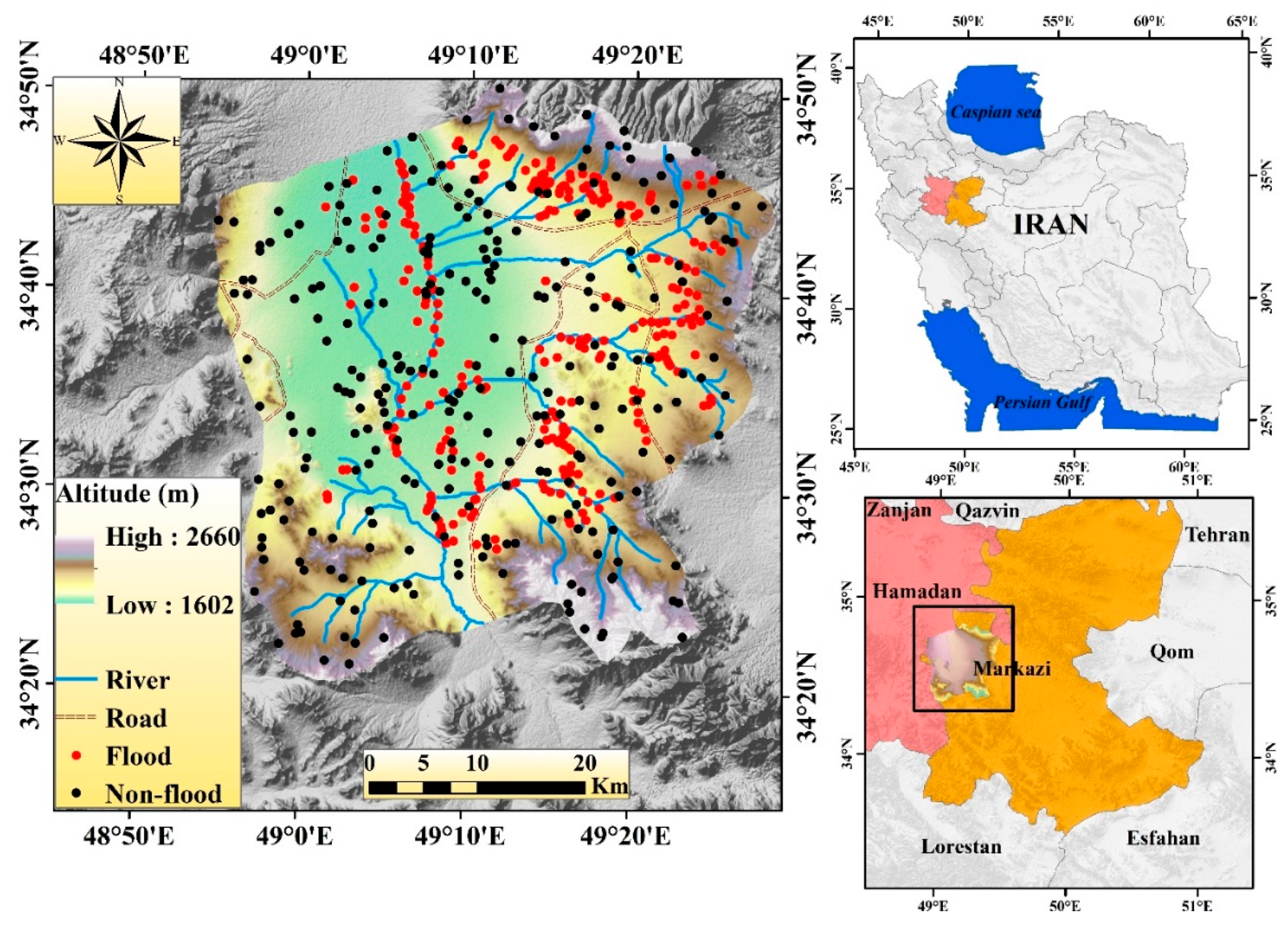
Figure 1. Location of the Kalvan watershed in Markazi and Hamadan Province, Iran.
Remotesensing 12 03568 g001
Figure 2. Methodological flow chart.
Remotesensing 12 03568 g002
Figure 3. Flash flood susceptibility conditioning factors: (a) Altitude, (b) slope, (c) aspect, (d) plan curvature, (e) profile curvature, (f) distance from river, (g) distance from road, (h) land use, (i) lithology, (j) soil depth, (k) rainfall, (l) stream power index (SPI), (m) topographic wetness index (TWI).
Remotesensing 12 03568 g003aRemotesensing 12 03568 g003b
Figure 4. Flash flood susceptibility map using the five models: (a) Boosted regression tree (BRT), (b) random forest (RF), (c) parallel random forest (PRF), (d) regularized random forest (RRF), and (e) extremely randomized trees (ERT).
Remotesensing 12 03568 g004aRemotesensing 12 03568 g004bRemotesensing 12 03568 g004c
Figure 5. Evaluation parameters in RRF mode.
Remotesensing 12 03568 g005
Figure 6. Evaluation parameters in ERT mode.
Remotesensing 12 03568 g006
Figure 7. The receiver operating characteristic (ROC) curve analysis for five flash flood susceptibility models using the validation dataset.
Remotesensing 12 03568 g007
Table 1. Multi-collinearity analysis to determine the linearity of the independent variables.
VariablesVIFTolerance
Altitude2.070.48
Slope2.440.41
Aspect1.070.93
Plan curvature1.570.64
Profile curvature1.440.69
Distance from river1.460.68
Distance from road1.380.72
Rainfall1.470.68
Land use1.540.65
Lithology2.030.49
Soil type1.490.67
SPI1.280.78
TWI1.670.60
Table 2. Flash flood susceptibility classes’ areas.
ModelsAreaSusceptibility Class
Very LowLowModerateHighVery High
BRTKm2100.7404.28442.73683.91425.13
%4.9019.6621.5233.2520.67
RFKm2618.49388.53440.21384.4225.12
%30.0718.9921.5618.7910.95
PRFKm2518.23440.96461.12396.72239.72
%25.2021.4422.4219.2911.65
RRFKm2608.89359.57466.56373.75247.98
%29.6017.4822.6818.1812.06
ERTKm2651.54431.14391.51332.72249.84
%31.6820.9619.0316.1812.15
Table 3. Predictive capability of piping models using train and test dataset.
ModelsStageParameters
SensitivitySpecificityPPVNPVAUC
BRTTrain0.860.620.690.810.83
Validation0.830.520.600.780.75
RFTrain0.840.780.820.800.89
Validation0.830.570.630.790.78
PRFTrain0.930.720.800.890.88
Validation0.820.590.640.790.79
RRFTrain0.770.800.820.740.87
Validation0.820.610.650.790.80
ERTTrain0.880.860.880.860.91
Validation0.810.660.670.790.82
Table 4. Variable importance analysis.
VariablesBRTRFPRFRRFERT
Altitude87.3681.8979.5336.9587.36
Slope86.2226.9526.9336.1586.22
Aspect18.2112.328.112.3414.79
Plan curvature22.3705.72022.37
Profile curvature29.529.111.635.3229.52
Distance from river10075.0374.8194.21100
Distance from road51.2839.1323.5124.7551.28
Rainfall94.9710010010094.97
Land use14.8810.7405.4214.88
Lithology63.2240.7237.6247.2163.22
Soil type14.4114.642.938.3414.41
SPI036.9130.7512.90
TWI69.0925.9217.6334.3469.09
Publisher’s Note: MDPI stays neutral with regard to jurisdictional claims in published maps and institutional affiliations.