Abstract
Garlic and winter wheat are major economic and grain crops in China, and their boundaries have increased substantially in recent decades. Updated and accurate garlic and winter wheat maps are critical for assessing their impacts on society and the environment. Remote sensing imagery can be used to monitor spatial and temporal changes in croplands such as winter wheat and maize. However, to our knowledge, few studies are focusing on garlic area mapping. Here, we proposed a method for coupling active and passive satellite imagery for the identification of both garlic and winter wheat in Northern China. First, we used passive satellite imagery (Sentinel-2 and Landsat-8 images) to extract winter crops (garlic and winter wheat) with high accuracy. Second, we applied active satellite imagery (Sentinel-1 images) to distinguish garlic from winter wheat. Third, we generated a map of the garlic and winter wheat by coupling the above two classification results. For the evaluation of classification, the overall accuracy was 95.97%, with a kappa coefficient of 0.94 by eighteen validation quadrats (3 km by 3 km). The user’s and producer’s accuracies of garlic are 95.83% and 95.85%, respectively; and for the winter wheat, these two accuracies are 97.20% and 97.45%, respectively. This study provides a practical exploration of targeted crop identification in mixed planting areas using multisource remote sensing data.
1. Introduction
Crop planting areas provides information for assessing food security and crop price [1,2,3]. Garlic and winter wheat are some of the primary economic and grain crops in China. However, obtaining the garlic and winter wheat planting area by the traditional census method needs a certain amount of human effort and cost [4]. Therefore, the timeliness is poor for these traditional methods. In addition, information regarding the planting area of garlic might be missing from government statistical data.
The remote sensing technique provides a very effective method for mapping crops [5,6,7], due to its fast response, and low cost [8,9,10]. However, there are still some difficulties for large-scale (e.g., regional or national scale) crops mapping. One of the main challenges is limited classification accuracy. For example, moderate resolution imaging spectroradiometer (MODIS) imagery has been the widely-applied remote sensing data source for large-scale crops mapping in previous studies [11,12,13]. The coarse spatial resolution (500/250 m) of MODIS imagery restricts the classification accuracy due to the issue of a large number of mixed pixels on MODIS imagery [13]. For instance, some researchers reported an overall accuracy of 88.86% when they mapped the winter wheat using MODIS data in China [2]. Therefore, we used Sentinel-2 and Landsat-8 optical multispectral images [14,15] with a spatial resolution of 10 m or 30 m to extract the garlic and winter wheat in the present study. When using these images, there is an issue associated with the vast volume of data and complex data processing. Image data volume is closely related to spatial resolution—the amount of data increases by four times with a spatial resolution increase of one time. Therefore, the data volume of Sentinel imagery (with a spatial resolution of 10 m) is approximately 2500 times that of MODIS imagery (with a spatial resolution of 500 m) for one band in the same study area. In previous studies, researchers usually selected a minor scale study area to reduce the difficulty associated with the massive amount of imagery preprocessing work [16,17].
Fortunately, the Google Earth Engine (GEE) cloud computing platform provides an effective solution for massive remote sensing data processing [18,19,20]. GEE datasets are preprocessed, and ready-to-use imagery data, which removes many barriers for data management [21]. More information about GEE is referred to by Gorelick et al. (2017). GEE has been widely used in remote sensing research on a large scale [22,23,24]. For instance, Jin et al. [25] studied smallholder maize area and yield with GEE. Hansen et al. [26] studied the global forest change using GEE. GEE cloud computing platform helps us to solve remote sensing big-data processing problems in this study.
Temporal profiles of vegetation indices (VIs) are widely used for crops mapping [27,28]. This is because crops have different phenology characteristics in their growing period and phenology is closely relevant to multi-temporal VIs [29,30]. During winter, the VIs of winter crops (includes garlic and winter wheat) are higher than those of other deciduous vegetation. During the maturity period of winter crops, VIs of winter crops are lower than those of other vegetation. Previous studies extracted winter crops based on this characteristic of winter crops and achieved good results [4,11]. However, it is challenging to build entire time series of VIs curves using Sentinel-2 and Landsat-8 imagery at a large scale because these images are easily influenced by clouds and its shadows [31,32]. Therefore, in the present study, we proposed an approach by compositing time series of Sentinel-2 and Landsat-8 images to solve the problem of inadequate optical imagery. We only identified winter crops from optical imagery without distinguishing garlic and winter wheat as they have similar phenology and spectral characteristics.
Sentinel-1 synthetic aperture radar (SAR) imagery has provided an unprecedented opportunity for crop monitoring due to their sensitivity of backscatter intensities to crop phenology and morphological development [33,34,35]. For example, Mandal et al. [33] proposed a dual-pol radar vegetation index based on Sentinel-1 images to characterize vegetation growth for the phenology of soybean and wheat. d’Andrimont et al. [36] detected the flowering phenology of oilseed rape using Sentinel-1 data. Chauhan et al. [37] monitored wheat lodging based on Sentinel-1 and Sentinel-2 imagery. Different types of crops have different canopy structures, and the canopy structure can be very different for different growth stages in one crop due to the leaves or stems from neighboring plants often intertwining [36,38]. The backscattering intensity of Sentinel-1 varies based on the change in the crop canopy structure [36]. Garlic and winter wheat have different canopy structures throughout their growth periods. Hence, we used Sentinel-1 images to identify garlic and winter wheat based on the winter crops map derived from optical imagery.
Recently, remote sensing classification methods have been rapidly developed and many advanced classification algorithms have emerged, e.g., random forest (RF) [39,40,41], support vector machines [42,43], deep learning [44,45], xTreme gradient boosting [41], and decision tree [46,47]. Among these methods, RF is a popular artificial intelligence algorithm, which is a combination of tree predictors [48]. These trees of RF are trained using the same features; however, various training sets are generated randomly from the original training data. After training, each tree assigns a class label to the test data. Finally, the results of all decision trees are fused and the majority of votes determine the class label for each land cover [42,49]. The excellent classification performance of RF has been proven by previous studies [50,51,52]. Additionally, the RF algorithm is encapsulated in GEE, and we can directly apply RF on the GEE cloud computing platform. Therefore, we selected the RF classifier to identify garlic and winter wheat.
In the present study, we focused on garlic and winter wheat classification in Northern China by coupling optical and Sentinel-1 SAR imagery. The aims of this study were to address the following three research questions: (1) Is the Sentinel-2 and Landsat-8 normalized difference vegetation index (NDVI) composition approach effective for winter crops mapping? (2) Are Sentinel-1 images effective for distinguishing between garlic and winter wheat? (3) Is the coupling of optical data and Sentinel-1 SAR data helpful for accurately identifying garlic and winter wheat?
2. Study Area
The study area is located in Northern China with a geographical range of 113.5° to 118.5°E and 34° to 36.6°N, as shown in Figure 1. The study area is one of the main producing areas of garlic and winter wheat in China. There are six China protected geographical indication products (CPGI, http://www.cpgi.org.cn/) for garlic in the study area, i.e., Zhongmou county, Qixian county, Jinxiang county, Lanling (Cangshan) county, Pizhou city, and Daming county (Figure 1b). In the study area, garlic and winter wheat have similar growth cycles and they are generally sown in October and harvested from May to June.
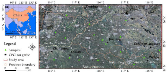
Figure 1.
(a) Location of the study area in China and (b) distribution of validation samples and the China protected geographical indication products (CPGI) for garlic.
3. Materials and Methods
The overall technical route of the study is shown in Figure 2. The workflow included five steps. First, we determined the time window based on the MODIS NDVI curves, which can reflect the phenological characteristics of winter crops (including garlic and winter wheat), and composited the time series of Sentinel-2 and Landsat-8 optical images. Optical image composition aims to enhance the image information of winter crops. Second, we extracted the winter crops using the optical composition imagery and the RF classification approach on GEE. Third, we composited the Sentinel-1 SAR imagery based on the time series of Sentinel-1 image curves, which can enhance the difference in image characteristics between garlic and winter wheat, and then distinguished the garlic and winter wheat based on the Sentinel-1 composition images by RF on GEE. Fourth, we yielded the intersection between optical classification results (from the second step) and Sentinel-1 classification results (from the third step) to achieve accurate identification of the garlic and winter wheat. Fifth, we validated the classification accuracy using the high spatial resolution image.
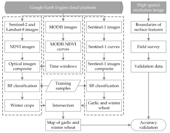
Figure 2.
Workflow for mapping garlic and winter wheat based on Sentinel-1 and Sentinel-2 imagery.
3.1. MODIS NDVI Curves and Composition of Sentinel-2 and Landsat-8 Images
To understand the phenological characteristics of garlic, winter wheat, and other surface features, their time series of MODIS NDVI curves from 6 September 2019 to 27 July 2020 were obtained based on the “MODIS/006/MOD09Q1” dataset from GEE. The MOD09Q1 data provided an estimate of the surface spectral reflectance of red and near-infrared (NIR) bands at 250 m resolution and have been corrected for atmospheric conditions. For per pixel location, a value was selected from all acquisitions within the 8 day composite based on high observation coverage, low view angle, the absence of clouds or cloud shadow, and aerosol loading. The MODIS NDVI images were computed using the following equation [53,54]:
where ρNIR is the reflectance of the NIR band and ρred is the reflectance of the red band.
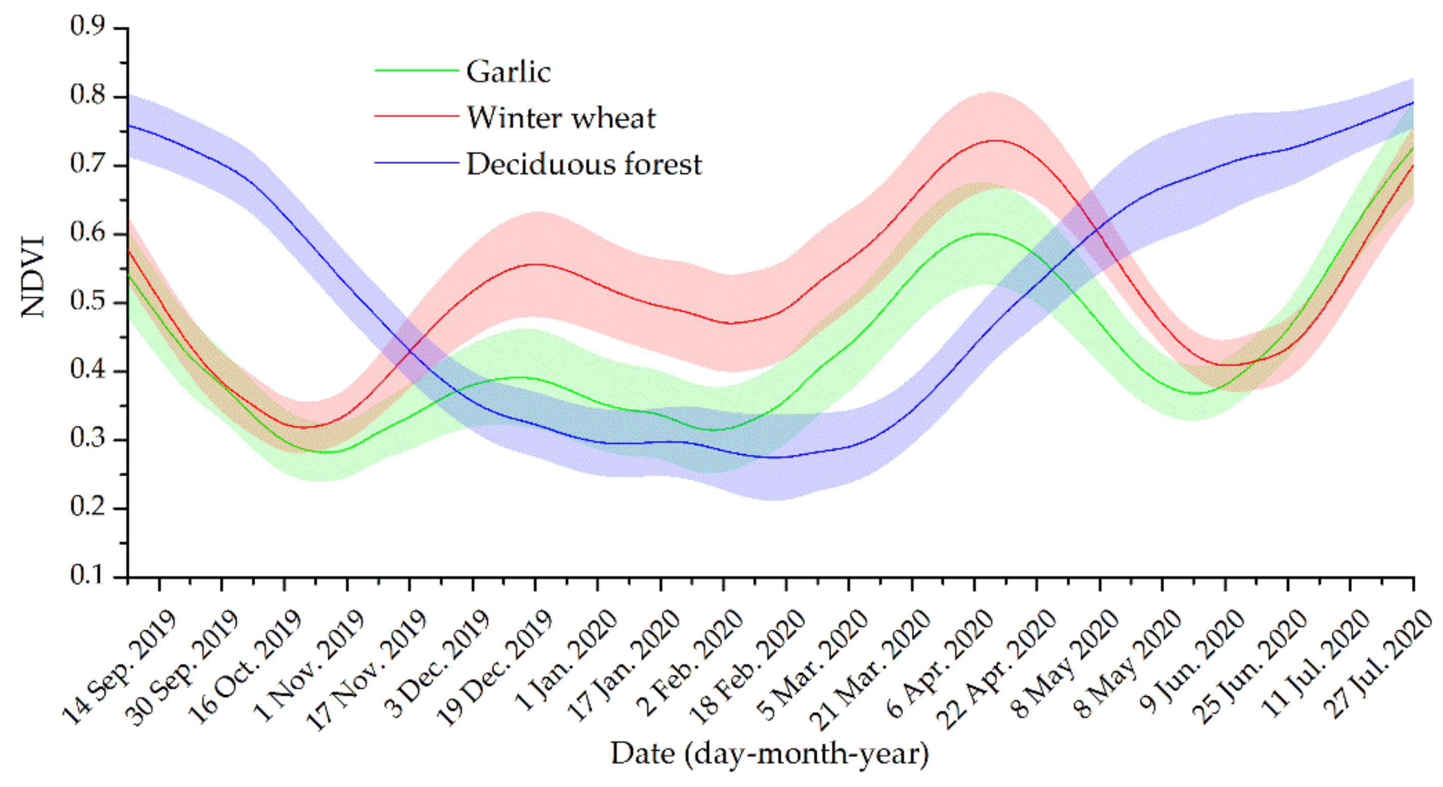
For time series MODIS NDVI images, the Savitzky–Golay filter [12,55] was applied to smooth the curves. Then, 1526 pixel sample curves of garlic, winter wheat, and deciduous forest were randomly selected from the time series MODIS NDVI images, as shown in Figure 3. The lines represent the mean NDVI value based on the samples, and the background color represents the standard deviation. Figure 3 illustrates that October is the sowing stage, and June is the harvest period for winter crops (garlic and winter wheat). Consequently, their NDVI values were lower than that of the deciduous forest in October and June, which was the time window of low NDVI values for winter crops. From December to March, winter crops reach the early or mid-life stages, and their green stems and leaves cover the ground, whereas this is the leaf-off stage for deciduous forests. Consequently, the NDVI value of winter crops was higher than that of the deciduous forest from December to March, which was the time window of high NDVI values for winter crops.

Figure 3.
Moderate resolution imaging spectroradiometer (MODIS) normalized difference vegetation index (NDVI) time series curves for different vegetation (i.e., garlic, winter wheat, and deciduous forest) in the study area from 6 September 2019 to 27 July 2020. The curves represent the mean NDVI value based on the samples. The background color represents the standard deviation for each type of vegetation NDVI curve.
In the study, we used Sentinel-2 and Landsat-8 images to extract winter crops. However, it was difficult to obtain a complete NDVI curve-like MODIS NDVI curve for any pixel based on Sentinel-2 and Landsat-8 imagery due to data availability, affected by weather conditions and differences in crop phenology. Therefore, we proposed an image composition method by using Sentinel-2 and Landsat-8 imagery to ensure that the image characteristics of the winter crops in the entire study areas were consistent. During the low NDVI value time window, i.e., from 1 October to 31 October 2019 and from 20 May to 30 June 2020, the minimum and median value composite images were computed based on the Sentinel-2 and Landsat-8 imagery. During the high NDVI value time window, i.e., from 1 December 2019 to 20 March 2020, only the maximum value composite image was computed based on the Sentinel-2 image. For example, there were multi NDVI values on every pixel location during the low NDVI value time window, we selected the minimum value among these NDVI values as the pixel value and used this method to traverse all pixel positions in turn in the study area. Thus, we obtained the minimum value composition image. The median and maximum value composition images were obtained in the same way. The three layer composition images were called optical composition images in the study.
The Sentinel-2 and Landsat-8 image collection were “COPERNICUS/S2” and “LANDSAT/LC08/C01/T1_TOA” on the GEE cloud platform, respectively, which were the top of atmosphere (TOA) reflectance production. To remove the influence of cloud cover, a mask cloud model from GEE was applied (more information on the mask cloud model can be found at https://code.earthengine.google.com/). The spatial resolutions of the Landsat-8 and Sentinel-2 images are 30 m and 10 m, respectively. Hence, the spatial resolution of Landsat-8 images was resampled to 10 m. The maximum value composition image only used the Sentinel-2 image, and its spatial resolution is 10 m, which ensured that the effective spatial resolution of the optical composition image reached 10 m.
3.2. Sentinel-1 Image Composition
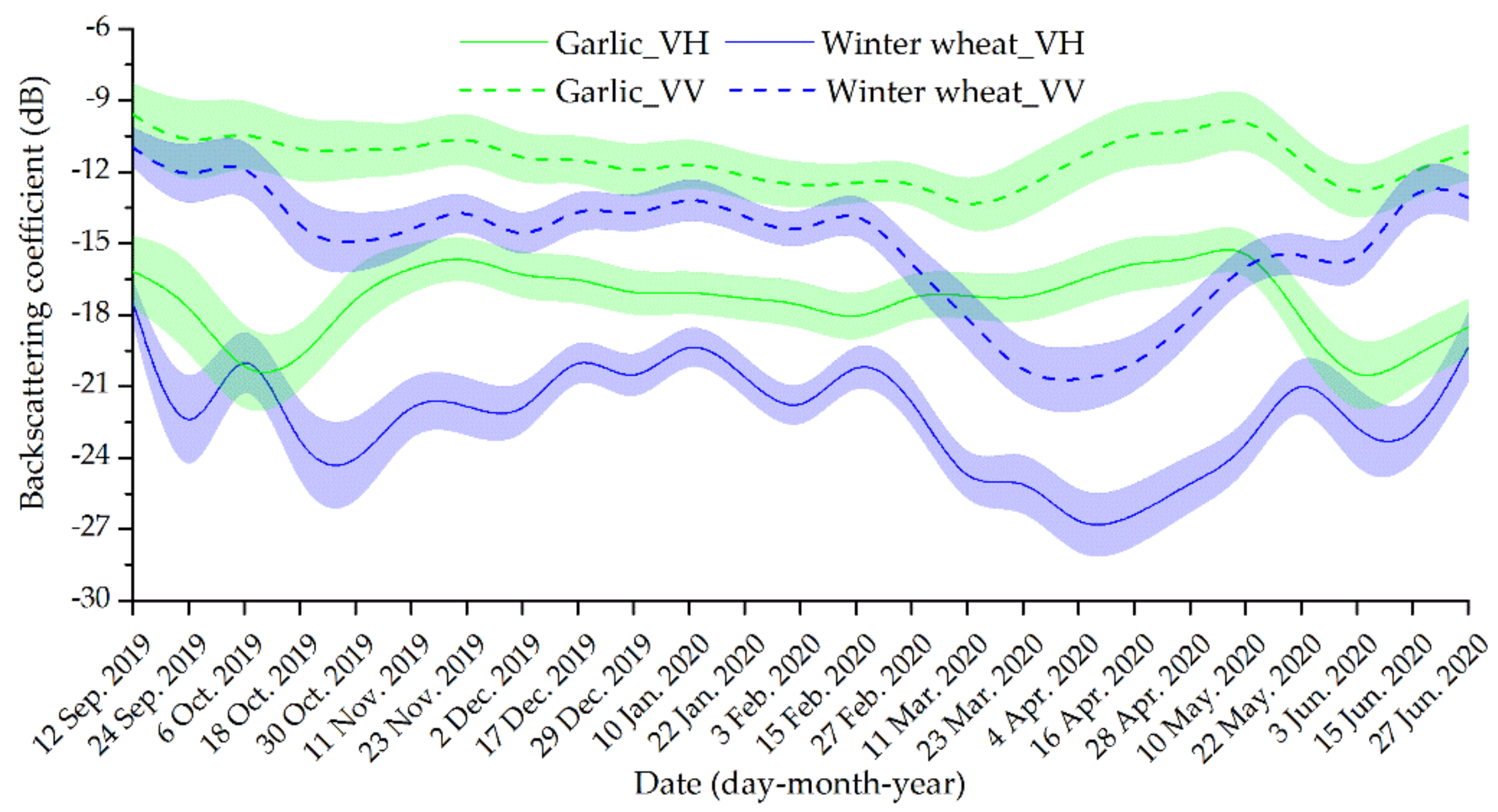
The time series of Sentinel-1 curves of garlic and winter wheat were plotted based on 1135 sample pixels, as shown in Figure 4, indicating a significant difference between garlic and wheat around April. The backscattering coefficient of winter wheat began to decrease significantly in March, reached a minimum value in early April, and then generally increased during April and May. However, garlic did not show the same changes in temporal characteristics.
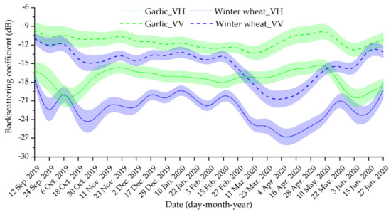
Figure 4.
Time series of Sentinel-1 curves for garlic and winter wheat. Green and blue refer to garlic and winter wheat, respectively. The dotted and solid lines represent the means of the backscattering coefficients of vertical- vertical (VV) and vertical-horizontal (VH) polarization images, respectively. The background color represents the standard deviation.
Therefore, three time windows were determined to enhance the difference between garlic and winter wheat and remove the difference of imaging date for different imagery strips. The first time window was from 1 January to 15 February 2020, the second time window was from 20 March to 20 April 2020, and the third time window was from 1 June to 15 June 2020. The median value composition images were computed in each time window for vertical-horizontal (VH) and vertical- vertical (VV) polarization imagery. Thus, the Sentinel-1 composition images were obtained.
3.3. Garlic and Winter Wheat Identification
First, a winter crops map (WCM) was obtained using the RF classification method based on the optical composition images (in Section 3.1) on the GEE cloud platform. The training samples included were 90 winter crops pixels and 59 other class pixels. The GEE codes, including the parameter of RF classifier and information on training samples, are shown in Appendix A. In the same way, garlic and winter wheat classification results (GWC) were obtained based on the Sentinel-1 composition images (in Section 3.2), and related GEE codes are shown in Appendix B.
Second, we defined that for a pixel that appeared as a winter crop on the WCM, if it was winter wheat on the GWC, then the pixel was winter wheat, or it was garlic. The remaining pixels were defined as the “other” category. Thus, we completed the coupling of optical and microwave classification results and created the final garlic and winter wheat map (FGWM).
3.4. Accuracy Validation
To achieve the objectivity of the accuracy validation and the operability of the sample selection, we selected eighteen quadrates of 3 × 3 km2, as shown in Figure 1. First, the boundaries of surface features within each quadrate were manually plotted based on the Google Earth imagery, and its spatial resolution was 1 m. Second, the attributes of surface features were identified from a field-based survey; then, these surface features were deemed to be ground-truth data. Third, we used the confusion matrix accuracy evaluation method to perform accuracy validation [56,57].
4. Results
4.1. Classification Results
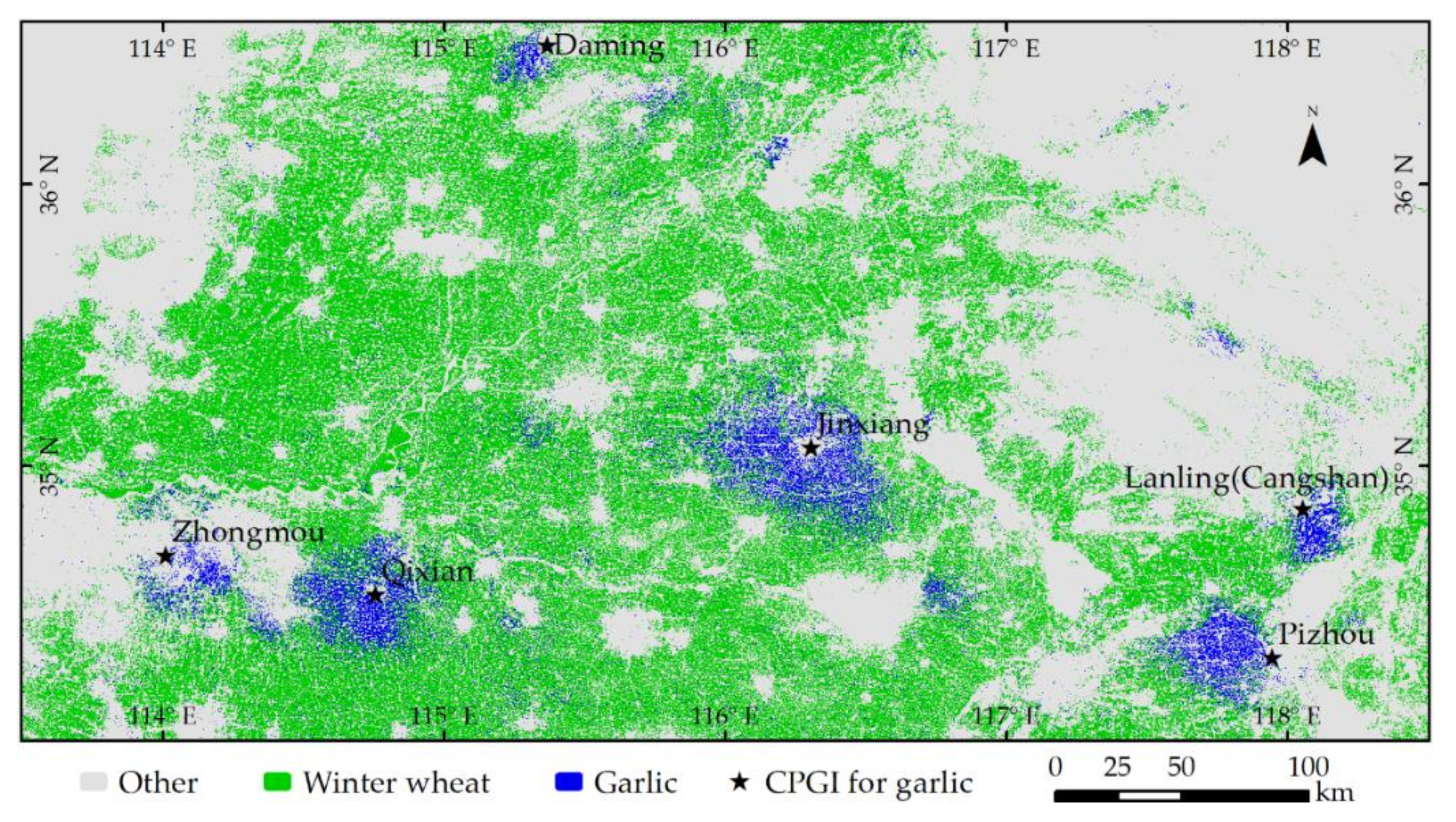
The WCM derived from the optical composition images as shown in Figure 5a and the GWC derived from Sentinel-1 SAR images as shown in Figure 5b illustrate that many non-garlic objects were incorrectly classified as garlic. In the WCM, the area of winter crops was 48,996.62 km2. In the GWC, the areas of the garlic and winter wheat were 53,182.22 km2 and 64,773.20 km2, respectively. Thus, the area of the winter crops (including garlic and winter wheat) that was extracted based on Sentinel-1 is larger than the area extracted based on the optical composition images.

Figure 5.
(a) Winter crops map (WCM) derived from optical composition images; (b) garlic and winter wheat classification results (GWC) derived from Sentinel-1 synthetic aperture radar (SAR) imagery.
The FGWM from 2020 (Figure 6) was obtained based on the WCM and GWC. In the study area, garlic had spatial characteristics of a concentrated distribution. For example, there were six major garlic planted regions in the study area, i.e., Zhongmou county, Qixian county, Jinxiang county, Lanling (Cangshan) county, Pizhou city, and Daming county. Among these regions, Jinxiang county had the largest garlic planting areas, with a value of 1091 km2. Winter wheat presented a continuous distribution of spatial characteristics and was the dominant winter crop in the study area. The planting areas of the garlic and winter wheat were 4664.03 km2 and 44,332.59 km2, respectively. The garlic planting areas was approximately one-tenth that of the winter wheat planting area, inconsistent with the results from the GWC solely using Sentinel-1 SAR images.

Figure 6.
The final garlic and winter wheat map (FGWM) from 2020 in the study area.
4.2. Accuracy
Based on the eighteen validation quadrats with an area of 3 km by 3 km, the classification accuracy for WCM and GWC is shown in Table 1 and Table 2. The overall accuracy was 96.08% with a kappa coefficient of 0.90 for WCM. Garlic and winter wheat were classified as winter crops because the optical composition images cannot distinguish them in the study. Therefore, we only reported the classification accuracy of winter crops in Table 1. The user’s and producer’s accuracies of winter crops classification results were 96.54% and 97.99%, respectively.

Table 1.
Results of accuracy validation for winter crops map (WCM).

Table 2.
Results of accuracy validation for garlic and winter wheat classification results (GWC).
For GWC, its overall accuracy was 73.62% with a kappa coefficient of 0.59. The user’s and producer’s accuracies of garlic classification results of GWC were 54.30% and 98.42%, respectively, and for winter wheat were 87.31% and 96.71%, respectively.
The overall accuracy was 95.97% with a kappa coefficient of 0.94 for the FGWM obtained from both WCM and GWC. As shown in Table 3, the user’s and producer’s accuracies of garlic classification results were 95.83% and 95.85%, respectively, and for winter wheat were 97.20% and 97.45%, respectively. The user’s accuracy and producer’s accuracy were similar for garlic and winter wheat classification results.

Table 3.
Results of accuracy validation for the final garlic and winter wheat map (FGWM).
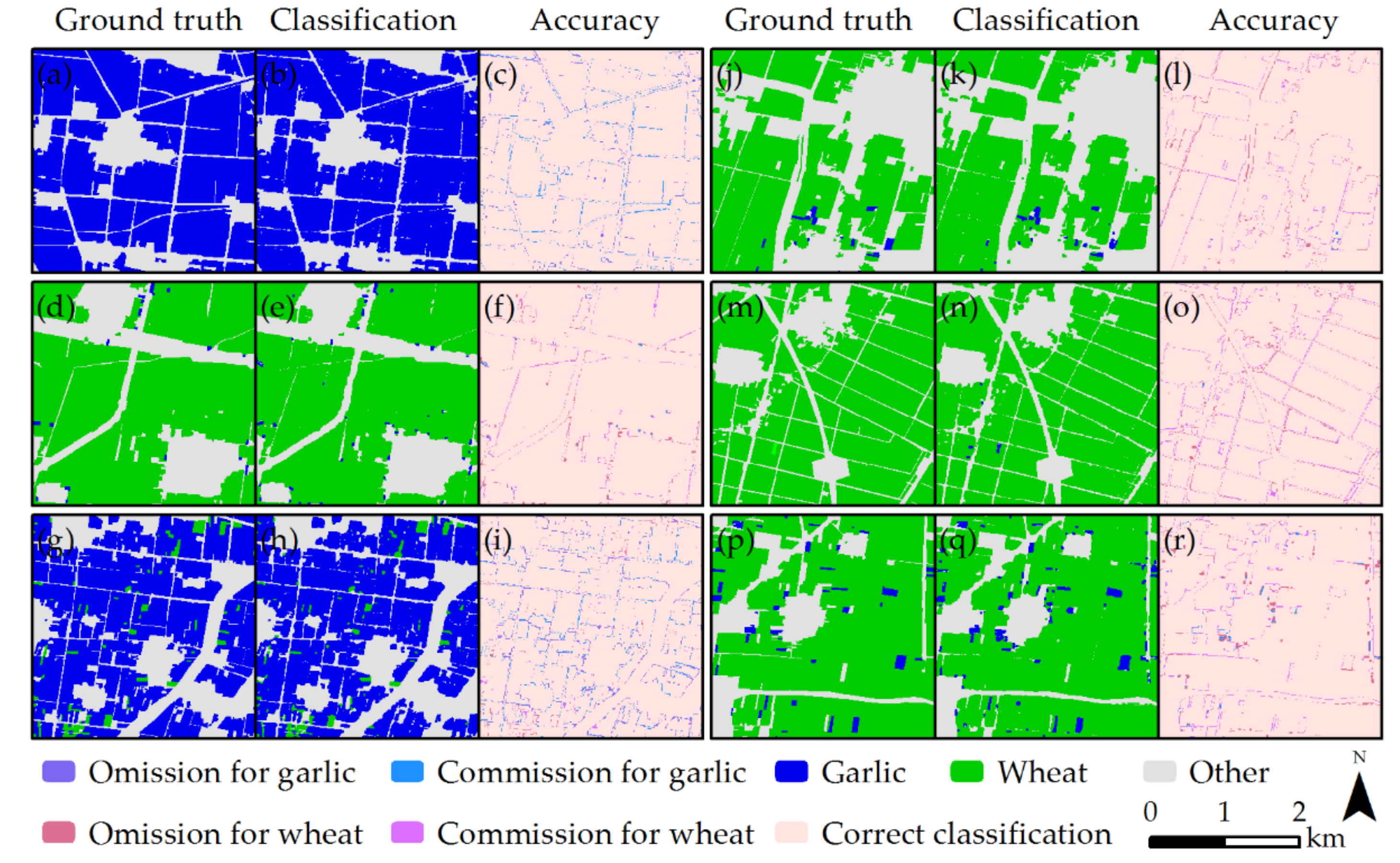
We randomly selected six validation quadrats to better understand the spatial distribution of correct and error classifications, as shown in Figure 7. The error classifications were mainly distributed at the boundaries of the different categories, which were strips with a width of one pixel. The texture of the ground features was well identified using our method. For example, the outlines of linear features (road and river) were clear on the classification map.
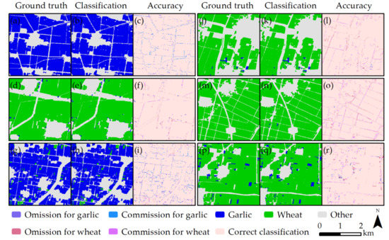
Figure 7.
Results of accuracy validation based on six validation quadrats with an area of 3 km by 3 km. (a,d,g,j,m,p) are the ground truth quadrats. (b,e,h,k,n,q) are the classification results for each quadrats. (c,f,i,l,o,r) are accuracy validation results.
5. Discussion
Garlic is an important economic crop and a necessity in people’s lives. Its planting area is large, nearly one-tenth that of winter wheat in the study area. An accurate acquisition of the planting areas of garlic is of great significance for forecasting the price of garlic and planting management. Nevertheless, limited studies have been undertaken on the simultaneous monitoring of garlic and winter wheat. Thus, the present study provides a useful exploration of the remote sensing identification of garlic and winter wheat using optical and Sentinel-1 SAR images.
The study area has a large east–west span, ranging from 113.5° to 118.5° E. Landsat-8 images require six imagery strips to cover the entire study area completely. The difference of imaging dates on different imagery strips can reach ten days, and the influence of cloud cover might exacerbate this difference [58]. Therefore, it can be difficult to find samples of NDVI temporal profiles to fully represent winter crops on all pixel positions based on the time series of Landsat-8 images, even for Sentinel-2 images [59]. This increased the challenges associated with crop identification. The imagery composition method proposed in the present study can effectively solve this problem. For example, there were three layers of images in the optical composition imagery, which significantly reduced the dependence on the number of cloud-free observations. Additionally, the optical composition imagery reduces the data redundancy and the dimension of imagery features for the winter crops, which helps improve the calculation efficiency [59].
Previous studies have verified that optical images have natural advantages when identifying vegetation [60,61,62], due to the unique spectral characteristics of vegetation [63]. Thereby, we obtained the potential and accurate maps of the winter crops (including garlic and winter wheat) using optical composition imagery, such as that shown in Figure 5a. However, optical images experience a lot of uncertainty when they are used to distinguish vegetation types. For example, different types of vegetation have similar spectral characteristics [59], and optical imagery is inevitably contaminated by clouds [64]. Therefore, it is difficult to accurately distinguish between garlic and winter wheat using optical imagery.
Figure 3 indicates that the NDVI of garlic was lower than that of winter wheat from December to May, particularly around January, which may help distinguish between garlic and winter wheat. The plant density of garlic was lower than that of winter wheat according to our survey, and the leaf area of garlic was lower than that of winter wheat during the same period. Thereby, theoretically, the NDVI of winter wheat was higher than that of garlic during this period. However, there were many mixed pixels for winter wheat, which caused the NDVI of winter wheat to decrease and become similar to that of garlic. Hence, it is almost impossible to distinguish garlic from winter wheat in practical applications using optical imagery.
In contrast to optical imagery, which are often contaminated by clouds and its shadows, SAR imagery is a reliable data source under all weather conditions [58]. SAR imagery is sensitive to plant structure [37,65,66]. As shown in Figure 4, the backscattering coefficient of winter wheat began to decrease significantly in March, reached a minimum value in early April, and then began to increase in both polarizations. It undergoes an elongation and booting stage from March to April for winter wheat [37,65]. Veloso et al. [67] stated that the observed backscatter was a combination of the ground backscatter, which was disturbed by soil moisture and surface roughness, and vegetation backscatter, which was destabilized by vegetation 3D structure. In addition, ground backscatter was dominant during the early and late growth of the crops, while vegetation backscatter generally dominates during the in-between growth stage. During the elongation and booting periods, the 3D structure of winter wheat changed significantly because of the increase in the number and length of stems [68]. This is the reason for the decrease in the backscattering coefficient. However, the garlic 3D structure did not experience these changes in characteristics.
The land use/cover classification accuracy using SAR imagery is generally lower than that of optical imagery with the same spatial resolution [59]. For example, many non-garlic crops were misclassified as garlic by only using Sentinel-1 SAR data, as seen in Figure 5b. The area of winter crops extracted from Sentinel-1 images was 117,955.42 km2, i.e., garlic was 53,182.22 km2, and winter wheat was 64,773.20 km2, which was 1.4 times greater than that extracted from the optical composition images. Therefore, combining optical and SAR imagery for crops mapping increases the overall accuracy compared to that of only employing optical or SAR imagery [58,69,70].
Compared to previous studies, our results have two contributions for crop mapping. First, higher accuracy (with overall accuracy of 95.97%), which was more 5% to 10% higher than that of some other studies. For example, Qiu et al. [2] reported an overall accuracy of 90.53% for winter wheat mapping and Yang et al. [7] reported overall accuracy from 82% to 88% for corn and rice mapping. Second, we distinguished garlic from winter wheat, which is important progress in the classification of types of winter crops. However, garlic, which has a similar growth cycle to winter wheat, is often neglected in some studies about winter crops mapping. For instance, Tao et al. [11] did not consider garlic in winter wheat mapping on the North China Plain, which limited map accuracy.
Although the accuracy of our result is satisfactory, there are still some uncertainties. For example, the difference between garlic and winter canola, which belongs to winter crops, on Sentinel-1 SAR imagery is unknown for the present paper, albeit the winter canola areas are few in the study area. Moreover, winter vegetables belong to winter crops, too. Comprehensive analysis of the imagery features of all different types of winter crops and improving the universality of garlic recognition methods are the directions for further research.
6. Conclusions
In the present study, by coupling the respective advantages of optical and microwave imagery, we achieved an accurate identification of garlic and winter wheat production in Northern China. Optical imagery can extract information on winter crops (including garlic and winter wheat), and microwave imagery can distinguish between garlic and winter wheat. In the study area, six major garlic producing areas were extracted with an overall accuracy of 95.97%. The accuracies of the user and producer for garlic are 95.83% and 95.85%, respectively, and that for winter wheat is 97.20% and 97.45%, respectively. These satisfactory accuracy data prove that the coupling of optical data and Sentinel-1 SAR data is helpful for accurately identifying garlic and winter wheat.
Optical imagery availability becomes limited when more than one cloud-free observation is required during some critical periods. In addition, the difference in the phenology of crops and imaging date means that the temporal profiles of crop image features are different. These interference factors restrict the classification accuracy. The proposed imagery composition scheme could reduce these limitations and is generally transferable to other study areas. The Sentinel-2 and Landsat-8 NDVI composition approach is an effective scheme for winter crops mapping.
Overall, the present study showed the great potential of coupling Sentinel-2 and Landsat-8 optical imagery and Sentinel-1 SAR imagery in improving the accuracy of the remotely sensed mapping of garlic and winter wheat.
Author Contributions
H.T., J.H., X.L. and Y.Q. conceived and designed the methodology; J.W. and J.P. performed the methodology; B.Z. and L.W. analyzed the data; and H.T. wrote the paper. All authors have read and agreed to the published version of the manuscript.
Funding
This research was funded by the China Postdoctoral Science Foundation, grant number [2019M662478], and National Demonstration Center for Experimental Environment and Planning Education (Henan University) Funding Project, grant number [2020HGSYJX009].
Conflicts of Interest
The authors declare that they have no known competing financial interests or personal relationships that could have appeared to influence the work reported in this paper.
Appendix A
The function of the following codes is to extract the overwintering crop map (OCM) using the random forest (RF) classification method based on the optical composition images on the Google Earth Engine (GEE) cloud computing platform. The codes runnable link is as follows: https://code.earthengine.google.com/a7f239ba8217a078ad707423cac1a9ac.
- var geometry = ee.Geometry.Rectangle([113.5,33.9,118.5,36.6]);
- var names = ‘optical_’;
- var month_min=[‘2019-10-1’,‘2019-11-1’,‘2020-5-20’,‘2020-7-1’];
- var month_max=[‘2019-12-1’,‘2020-3-20’];
- function maskS2clouds(image) {
- var qa = image.select(‘QA60’);
- var cloudBitMask = 1 << 10;
- var cirrusBitMask = 1 << 11;
- var mask = qa.bitwiseAnd(cloudBitMask).eq(0).and(qa.bitwiseAnd(cirrusBitMask).eq(0));
- return image.updateMask(mask).divide(10000).select(“B.*”).copyProperties(image, [“system:time_start”])}
- var maskL8 = function(image) {
- var qa = image.select(‘BQA’);
- var mask = qa.bitwiseAnd(1 << 4).eq(0);
- return image.updateMask(mask);};
- var kernel = ee.Kernel.square({radius: 1});
- var medianFilter = function(image){return image.addBands(image.focal_median({kernel: kernel, iterations: 1}))};
- var addNDVI = function(image){
- return image.addBands(image.normalizedDifference([‘nir’,’red’]).rename(‘ndvi’));};
- var s2b10 = [‘B2’, ‘B3’, ‘B4’, ‘B8’];
- var lan8 = [‘B2’, ‘B3’, ‘B4’, ‘B5’];
- var STD_NAMES_s2 = [‘blue’,‘green’,‘red’,‘nir’];
- var percentiles =[0,10,20,30,40,50,60,70,80,90,100];
- var sen2_1 = ee.ImageCollection(‘COPERNICUS/S2’)
- .filterDate(month_min[0], month_min[1])
- .filterBounds(geometry)
- .filter(ee.Filter.lt(‘CLOUDY_PIXEL_PERCENTAGE’, 20))
- .map(maskS2clouds)
- .select(s2b10,STD_NAMES_s2);
- var sen2_2 = ee.ImageCollection(‘COPERNICUS/S2’)
- .filterDate(month_min[2], month_min[3])
- .filterBounds(geometry)
- .filter(ee.Filter.lt(‘CLOUDY_PIXEL_PERCENTAGE’, 20))
- .map(maskS2clouds)
- .select(s2b10,STD_NAMES_s2);
- var lan8_1 = ee.ImageCollection(‘LANDSAT/LC08/C01/T1_TOA’)
- .filterDate(month_min[0], month_min[1])
- .filterBounds(geometry)
- .map(maskL8)
- .select(lan8,STD_NAMES_s2);
- var lan8_2 = ee.ImageCollection(‘LANDSAT/LC08/C01/T1_TOA’)
- .filterDate(month_min[2], month_min[3])
- .filterBounds(geometry)
- .map(maskL8)
- .select(lan8,STD_NAMES_s2);
- var lan8_min = ee.ImageCollection(lan8_1.merge(lan8_2));
- var sen2_min = ee.ImageCollection(sen2_1.merge(sen2_2).merge(lan8_min));
- var sen2_ndvi_min = sen2_min.map(addNDVI).select(‘ndvi’).min().clip(geometry);
- var sen2_ndvi_med = sen2_min.map(addNDVI).select(‘ndvi’).median().clip(geometry);
- var sen2_max = ee.ImageCollection(‘COPERNICUS/S2’)
- .filterDate(month_max[0], month_max[1])
- .filterBounds(geometry)
- .filter(ee.Filter.lt(‘CLOUDY_PIXEL_PERCENTAGE’, 20))
- .map(maskS2clouds)
- .select(s2b10,STD_NAMES_s2);
- var sen2_ndvi_max = sen2_max.map(addNDVI).select(‘ndvi’).max().clip(geometry);
- var sen_comp = sen2_ndvi_max.addBands(sen2_ndvi_min).addBands(sen2_ndvi_med);
- Map.addLayer(sen_comp,{min: 0, max: 0.8},‘sen_comp’);
- var features = [winter,other];
- var sample = ee.FeatureCollection(features);
- var training = sen_comp.sampleRegions({collection:sample, properties: [‘class’], scale: 10});
- var rf_classifier = ee.Classifier.randomForest(100).train(training, ‘class’);
- var RF_classified = sen_comp.classify(rf_classifier);
- var RF_classified = ee.Image(RF_classified).int8();
- Map.addLayer(RF_classified,{min: 0, max:2},‘RF_classified’);
- Export.image.toDrive({
- image:RF_classified,
- description:names+‘ndvi_class’,
- fileNamePrefix: names+‘ndvi_class’,
- scale: 10,
- region: geometry,
- maxPixels: 900000000000});
Appendix B
The function of the following codes is to extract the garlic and winter wheat classification results (GWC) using the RF classification method based on the Sentinel-1 composition images on the GEE cloud computing platform. The codes runnable link is as follows: https://code.earthengine.google.com/0bf373de1c9fd3750862bbd29a59651b.
- var geometry = ee.Geometry.Rectangle([113.5,33.9,118.5,37]);var names = ‘s1_’;
- var month1=[‘2020-1-1’,‘2020-2-16’];
- var month2=[‘2020-4-1’,‘2020-5-1’];
- var month3=[‘2020-6-1’,‘2020-6-16’];
- var nodataMask1 = function(img) { var score1 =img.select(‘VH’); return img.updateMask(score1.gt(-30)); };
- var nodataMask2 = function(img) { var score2 =img.select(‘VV’); return img.updateMask(score2.gt(-28)); };
- var kernel = ee.Kernel.square({radius: 1});
- var medianFilter = function(image){ return image.addBands(image.focal_median({kernel: kernel, iterations: 1}))};
- var s1_1 = ee.ImageCollection(‘COPERNICUS/S1_GRD’)
- .filterBounds(geometry)
- .filterDate(month1[0], month1[1])
- .filter(ee.Filter.listContains(‘transmitterReceiverPolarisation’, ‘VH’))
- .filter(ee.Filter.listContains(‘transmitterReceiverPolarisation’, ‘VV’))
- .map(nodataMask1)
- .map(nodataMask2)
- .map(medianFilter);
- var s1_1_vh = s1_1.select(‘VH’).median();
- var s1_1_vv = s1_1.select(‘VV’).median();
- var s1_2 = ee.ImageCollection(‘COPERNICUS/S1_GRD’)
- .filterBounds(geometry)
- .filterDate(month2[0], month2[1])
- .filter(ee.Filter.listContains(‘transmitterReceiverPolarisation’, ‘VH’))
- .filter(ee.Filter.listContains(‘transmitterReceiverPolarisation’, ‘VV’))
- .map(nodataMask1)
- .map(nodataMask2)
- .map(medianFilter);
- var s1_2_vh = s1_2.select(‘VH’).median();
- var s1_2_vv = s1_2.select(‘VV’).median();
- var s1_3 = ee.ImageCollection(‘COPERNICUS/S1_GRD’)
- .filterBounds(geometry)
- .filterDate(month3[0], month3[1])
- .filter(ee.Filter.listContains(‘transmitterReceiverPolarisation’, ‘VH’))
- .filter(ee.Filter.listContains(‘transmitterReceiverPolarisation’, ‘VV’))
- .map(nodataMask1)
- .map(nodataMask2)
- .map(medianFilter);
- var s1_3_vh = s1_3.select(‘VH’).median();
- var s1_3_vv = s1_3.select(‘VV’).median();
- var s1_img = s1_1_vv.addBands(s1_2_vv).addBands(s1_1_vh).addBands(s1_2_vh).addBands(s1_3_vh);
- Map.addLayer(s1_img,{min: -30, max: 0},‘s1_img’);
- Map.centerObject(s1_img, 7);
- var features = [garlic,wheat,other]
- var sample = ee.FeatureCollection(features)
- var training = s1_img.sampleRegions({ collection:sample, properties: [‘class’], scale: 10});
- var rf_classifier = ee.Classifier.randomForest(100).train(training, ‘class’);
- var RF_classified = s1_img.classify(rf_classifier);
- var RF_classified = ee.Image(RF_classified).int8();
- Map.addLayer(RF_classified,{min: 1, max:3},‘RF_classified’);
- Export.image.toDrive({
- image:RF_classified,
- description:names+‘sar_class’,
- fileNamePrefix:names+‘sar_class’,
- scale: 10,
- region: geometry,
- maxPixels: 900000000000});
References
- Xie, Y.; Wang, P.X.; Bai, X.J.; Khan, J.; Zhang, S.Y.; Li, L.; Wang, L. Assimilation of the leaf area index and vegetation temperature condition index for winter wheat yield estimation using landsat imagery and the ceres-wheat model. Agric. Forest Meteorol. 2017, 246, 194–206. [Google Scholar] [CrossRef]
- Qiu, B.W.; Luo, Y.H.; Tang, Z.H.; Chen, C.C.; Lu, D.F.; Huang, H.Y.; Chen, Y.Z.; Chen, N.; Xu, W.M. Winter wheat mapping combining variations before and after estimated heading dates. ISPRS J. Photogramm. Remote Sens. 2017, 123, 35–46. [Google Scholar] [CrossRef]
- Huang, J.; Tian, L.; Liang, S.; Ma, H.; Becker-Reshef, I.; Huang, Y.; Su, W.; Zhang, X.; Zhu, D.; Wu, W. Improving winter wheat yield estimation by assimilation of the leaf area index from landsat tm and modis data into the wofost model. Agric. Forest Meteorol. 2015, 204, 106–121. [Google Scholar] [CrossRef]
- Tian, H.F.; Huang, N.; Niu, Z.; Qin, Y.C.; Pei, J.; Wang, J. Mapping Winter Crops in China with Multi-Source Satellite Imagery and Phenology-Based Algorithm. Remote Sens. 2019, 11, 820. [Google Scholar] [CrossRef]
- Ma, Y.P.; Wang, S.L.; Zhang, L.; Hou, Y.Y.; Zhuang, L.W.; He, Y.B.; Wang, F.T. Monitoring winter wheat growth in North China by combining a crop model and remote sensing data. Int. J. Appl. Earth Obs. Geoinf. 2008, 10, 426–437. [Google Scholar] [CrossRef]
- Dominguez, J.A.; Kumhalova, J.; Novak, P. Winter oilseed rape and winter wheat growth prediction using remote sensing methods. Plant Soil Environ. 2015, 61, 410–416. [Google Scholar] [CrossRef]
- Yang, N.; Liu, D.; Feng, Q.; Xiong, Q.; Zhang, L.; Ren, T.; Zhao, Y.; Zhu, D.; Huang, J. Large-Scale Crop Mapping Based on Machine Learning and Parallel Computation with Grids. Remote Sens. 2019, 11, 1500. [Google Scholar] [CrossRef]
- Franke, J.; Menz, G. Multi-temporal wheat disease detection by multi-spectral remote sensing. Precis. Agric. 2007, 8, 161–172. [Google Scholar] [CrossRef]
- Tian, H.F.; Wu, M.Q.; Wang, L.; Niu, Z. Mapping Early, Middle and Late Rice Extent Using Sentinel-1A and Landsat-8 Data in the Poyang Lake Plain, China. Sensors 2018, 18, 185. [Google Scholar] [CrossRef]
- Wang, J.; Wu, C.; Wang, X.; Zhang, X. A new algorithm for the estimation of leaf unfolding date using MODIS data over China’s terrestrial ecosystems. ISPRS J. Photogramm. Remote Sens. 2019, 149, 77–90. [Google Scholar] [CrossRef]
- Tao, J.B.; Wu, W.B.; Zhou, Y.; Wang, Y.; Jiang, Y. Mapping winter wheat using phenological feature of peak before winter on the North China Plain based on time-series MODIS data. J. Integr. Agric. 2017, 16, 348–359. [Google Scholar] [CrossRef]
- Sun, H.S.; Xu, A.G.; Lin, H.; Zhang, L.P.; Mei, Y. Winter wheat mapping using temporal signatures of MODIS vegetation index data. Int. J. Remote Sens. 2012, 33, 5026–5042. [Google Scholar] [CrossRef]
- Pan, Y.Z.; Li, L.; Zhang, J.S.; Liang, S.L.; Zhu, X.F.; Sulla-Menashe, D. Winter wheat area estimation from MODIS-EVI time series data using the Crop Proportion Phenology Index. Remote Sens. Environ. 2012, 119, 232–242. [Google Scholar] [CrossRef]
- Pasqualotto, N.; Delegido, J.; Van Wittenberghe, S.; Rinaldi, M.; Moreno, J. Multi-Crop Green LAI Estimation with a New Simple Sentinel-2 LAI Index (SeLI). Sensors 2019, 19, 904. [Google Scholar] [CrossRef] [PubMed]
- Zhu, J.; Pan, Z.W.; Wang, H.; Huang, P.J.; Sun, J.L.; Qin, F.; Liu, Z.Z. An Improved Multi-temporal and Multi-feature Tea Plantation Identification Method Using Sentinel-2 Imagery. Sensors 2019, 19, 2087. [Google Scholar] [CrossRef]
- Ahmadian, N.; Ghasemi, S.; Wigneron, J.P.; Zolitz, R. Comprehensive study of the biophysical parameters of agricultural crops based on assessing Landsat 8 OLI and Landsat 7 ETM+ vegetation indices. Gisci. Remote Sens. 2016, 53, 337–359. [Google Scholar] [CrossRef]
- Ozelkan, E.; Chen, G.; Ustundag, B.B. Multiscale object-based drought monitoring and comparison in rainfed and irrigated agriculture from Landsat 8 OLI imagery. Int. J. Appl. Earth Obs. Geoinf. 2016, 44, 159–170. [Google Scholar] [CrossRef]
- Xiong, J.; Thenkabail, P.S.; Gumma, M.K.; Teluguntla, P.; Poehnelt, J.; Congalton, R.G.; Yadav, K.; Thau, D. Automated cropland mapping of continental Africa using Google Earth Engine cloud computing. ISPRS J. Photogramm. Remote Sens. 2017, 126, 225–244. [Google Scholar] [CrossRef]
- Chen, F.; Zhang, M.M.; Tian, B.S.; Li, Z. Extraction of Glacial Lake Outlines in Tibet Plateau Using Landsat 8 Imagery and Google Earth Engine. IEEE J. Sel. Top. Appl. Earth Obs. Remote Sens. 2017, 10, 4002–4009. [Google Scholar] [CrossRef]
- Teluguntla, P.; Thenkabail, P.S.; Oliphant, A.; Xiong, J.; Gumma, M.K.; Congalton, R.G.; Yadav, K.; Huete, A. A 30-m landsat-derived cropland extent product of Australia and China using random forest machine learning algorithm on Google Earth Engine cloud computing platform. ISPRS J. Photogramm. Remote Sens. 2018, 144, 325–340. [Google Scholar] [CrossRef]
- Gorelick, N.; Hancher, M.; Dixon, M.; Ilyushchenko, S.; Thau, D.; Moore, R. Google Earth Engine: Planetary-scale geospatial analysis for everyone. Remote Sens. Environ. 2017, 202, 18–27. [Google Scholar] [CrossRef]
- Traganos, D.; Aggarwal, B.; Poursanidis, D.; Topouzelis, K.; Chrysoulakis, N.; Reinartz, P. Towards Global-Scale Seagrass Mapping and Monitoring Using Sentinel-2 on Google Earth Engine: The Case Study of the Aegean and Ionian Seas. Remote Sens. 2018, 10, 1227. [Google Scholar] [CrossRef]
- Tsai, Y.H.; Stow, D.; Chen, H.L.; Lewison, R.; An, L.; Shi, L. Mapping Vegetation and Land Use Types in Fanjingshan National Nature Reserve Using Google Earth Engine. Remote Sens. 2018, 10, 927. [Google Scholar] [CrossRef]
- Pei, J.; Wang, L.; Wang, X.; Niu, Z.; Cao, J. Time Series of Landsat Imagery Shows Vegetation Recovery in Two Fragile Karst Watersheds in Southwest China from 1988 to 2016. Remote Sens. 2019, 11, 2044. [Google Scholar] [CrossRef]
- Jin, Z.N.; Azzari, G.; You, C.; Di Tommaso, S.; Aston, S.; Burke, M.; Lobell, D.B. Smallholder maize area and yield mapping at national scales with Google Earth Engine. Remote Sens. Environ. 2019, 228, 115–128. [Google Scholar] [CrossRef]
- Hansen, M.C.; Potapov, P.V.; Moore, R.; Hancher, M.; Turubanova, S.A.; Tyukavina, A.; Thau, D.; Stehman, S.V.; Goetz, S.J.; Loveland, T.R.; et al. High-Resolution Global Maps of 21st-Century Forest Cover Change. Science 2013, 342, 850–853. [Google Scholar] [CrossRef]
- Sakamoto, T.; Yokozawa, M.; Toritani, H.; Shibayama, M.; Ishitsuka, N.; Ohno, H. A crop phenology detection method using time-series MODIS data. Remote Sens. Environ. 2005, 96, 366–374. [Google Scholar] [CrossRef]
- Cai, Y.P.; Guan, K.Y.; Peng, J.; Wang, S.W.; Seifert, C.; Wardlow, B.; Li, Z. A high-performance and in-season classification system of field-level crop types using time-series Landsat data and a machine learning approach. Remote Sens. Environ. 2018, 210, 35–47. [Google Scholar] [CrossRef]
- Sakamoto, T.; Wardlow, B.D.; Gitelson, A.A.; Verma, S.B.; Suyker, A.E.; Arkebauer, T.J. A Two-Step Filtering approach for detecting maize and soybean phenology with time-series MODIS data. Remote Sens. Environ. 2010, 114, 2146–2159. [Google Scholar] [CrossRef]
- Wang, J.; Wu, C.; Zhang, C.; Ju, W.; Wang, X.; Chen, Z.; Fang, B. Improved modeling of gross primary productivity (GPP) by better representation of plant phenological indicators from remote sensing using a process model. Ecol. Indic. 2018, 88, 332–340. [Google Scholar] [CrossRef]
- Tian, H.F.; Li, W.; Wu, M.Q.; Huang, N.; Li, G.D.; Li, X.; Niu, Z. Dynamic Monitoring of the Largest Freshwater Lake in China Using a New Water Index Derived from High Spatiotemporal Resolution Sentinel-1A Data. Remote Sens. 2017, 9, 521. [Google Scholar] [CrossRef]
- Zhu, Z.; Woodcock, C.E. Object-based cloud and cloud shadow detection in Landsat imagery. Remote Sens. Environ. 2012, 118, 83–94. [Google Scholar] [CrossRef]
- Mandal, D.; Kumar, V.; Ratha, D.; Dey, S.; Bhattacharya, A.; Lopez-Sanchez, J.M.; McNairn, H.; Rao, Y.S. Dual polarimetric radar vegetation index for crop growth monitoring using sentinel-1 SAR data. Remote Sens. Environ. 2020, 247, 111954. [Google Scholar] [CrossRef]
- Fikriyah, V.N.; Darvishzadeh, R.; Laborte, A.; Khan, N.I.; Nelson, A. Discriminating transplanted and direct seeded rice using Sentinel-1 intensity data. Int. J. Appl. Earth Obs. Geoinf. 2019, 76, 143–153. [Google Scholar] [CrossRef]
- Singha, M.; Dong, J.W.; Zhang, G.L.; Xiao, X.M. High resolution paddy rice maps in cloud-prone Bangladesh and Northeast India using Sentinel-1 data. Sci. Data 2019, 6, 26. [Google Scholar] [CrossRef] [PubMed]
- d’Andrimont, R.; Taymans, M.; Lemoine, G.; Ceglar, A.; Yordanov, M.; van der Velde, M. Detecting flowering phenology in oil seed rape parcels with Sentinel-1 and-2 time series. Remote Sens. Environ. 2020, 239, 111660. [Google Scholar] [CrossRef] [PubMed]
- Chauhan, S.; Darvishzadeh, R.; Lu, Y.; Boschetti, M.; Nelson, A. Understanding wheat lodging using multi-temporal Sentinel-1 and Sentinel-2 data. Remote Sens. Environ. 2020, 243. [Google Scholar] [CrossRef]
- Cable, J.W.; Kovacs, J.M.; Jiao, X.F.; Shang, J.L. Agricultural Monitoring in Northeastern Ontario, Canada, Using Multi-Temporal Polarimetric RADARSAT-2 Data. Remote Sens. 2014, 6, 2343–2371. [Google Scholar] [CrossRef]
- Luo, Y.M.; Huang, D.T.; Liu, P.Z.; Feng, H.M. An novel random forests and its application to the classification of mangroves remote sensing image. Multimed. Tools Appl. 2016, 75, 9707–9722. [Google Scholar] [CrossRef]
- Yu, Y.; Li, M.Z.; Fu, Y. Forest type identification by random forest classification combined with SPOT and multitemporal SAR data. J. For. Res. 2018, 29, 1407–1414. [Google Scholar] [CrossRef]
- Abdullah, A.Y.M.; Masrur, A.; Adnan, M.S.G.; Al Baky, M.A.; Hassan, Q.K.; Dewan, A. Spatio-Temporal Patterns of Land Use/Land Cover Change in the Heterogeneous Coastal Region of Bangladesh between 1990 and 2017. Remote Sens. 2019, 11, 790. [Google Scholar] [CrossRef]
- Bangira, T.; Alfieri, S.M.; Menenti, M.; van Niekerk, A. Comparing Thresholding with Machine Learning Classifiers for Mapping Complex Water. Remote Sens. 2019, 11, 1351. [Google Scholar] [CrossRef]
- Mountrakis, G.; Im, J.; Ogole, C. Support vector machines in remote sensing: A review. ISPRS J. Photogramm. Remote Sens. 2011, 66, 247–259. [Google Scholar] [CrossRef]
- Reichstein, M.; Camps-Valls, G.; Stevens, B.; Jung, M.; Denzler, J.; Carvalhais, N.; Prabhat. Deep learning and process understanding for data-driven Earth system science. Nature 2019, 566, 195–204. [Google Scholar] [CrossRef] [PubMed]
- Wang, X.; Huang, J.; Feng, Q.; Yin, D. Winter Wheat Yield Prediction at County Level and Uncertainty Analysis in Main Wheat-Producing Regions of China with Deep Learning Approaches. Remote Sens. 2020, 12, 1744. [Google Scholar] [CrossRef]
- Sun, D.L.; Yu, Y.Y.; Goldberg, M.D. Deriving Water Fraction and Flood Maps From MODIS Images Using a Decision Tree Approach. IEEE J. Sel. Top. Appl. Earth Obs. Remote Sens. 2011, 4, 814–825. [Google Scholar] [CrossRef]
- Xu, M.; Watanachaturaporn, P.; Varshney, P.K.; Arora, M.K. Decision tree regression for soft classification of remote sensing data. Remote Sens. Environ. 2005, 97, 322–336. [Google Scholar] [CrossRef]
- Li, L.Y.; Chen, Y.; Xu, T.B.; Shi, K.F.; Liu, R.; Huang, C.; Lu, B.B.; Meng, L.K. Remote Sensing of Wetland Flooding at a Sub-Pixel Scale Based on Random Forests and Spatial Attraction Models. Remote Sens. 2019, 11, 1231. [Google Scholar] [CrossRef]
- Amani, M.; Salehi, B.; Mahdavi, S.; Granger, J.; Brisco, B. Wetland classification in Newfoundland and Labrador using multi-source SAR and optical data integration. Gisci. Remote Sens. 2017, 54, 779–796. [Google Scholar] [CrossRef]
- Houborg, R.; McCabe, M.F. A hybrid training approach for leaf area index estimation via Cubist and random forests machine-learning. ISPRS J. Photogramm. Remote Sens. 2018, 135, 173–188. [Google Scholar] [CrossRef]
- Breiman, L. Random forests. Mach. Learn. 2001, 45, 5–32. [Google Scholar] [CrossRef]
- Rodriguez-Galiano, V.F.; Ghimire, B.; Rogan, J.; Chica-Olmo, M.; Rigol-Sanchez, J.P. An assessment of the effectiveness of a random forest classifier for land-cover classification. ISPRS J. Photogramm. Remote Sens. 2012, 67, 93–104. [Google Scholar] [CrossRef]
- Huete, A.; Didan, K.; Miura, T.; Rodriguez, E.P.; Gao, X.; Ferreira, L.G. Overview of the radiometric and biophysical performance of the MODIS vegetation indices. Remote Sens. Environ. 2002, 83, 195–213. [Google Scholar] [CrossRef]
- Lunetta, R.S.; Knight, J.F.; Ediriwickrema, J.; Lyon, J.G.; Worthy, L.D. Land-cover change detection using multi-temporal MODIS NDVI data. Remote Sens. Environ. 2006, 105, 142–154. [Google Scholar] [CrossRef]
- Chen, J.; Jonsson, P.; Tamura, M.; Gu, Z.H.; Matsushita, B.; Eklundh, L. A simple method for reconstructing a high-quality NDVI time-series data set based on the Savitzky-Golay filter. Remote Sens. Environ. 2004, 91, 332–344. [Google Scholar] [CrossRef]
- Card, D.H. Using known map category marginal frequencies to improve estimates of thematic map accuracy. Photogramm. Eng. Remote Sens. 1982, 48, 431–439. [Google Scholar]
- Olofsson, P.; Foody, G.M.; Stehman, S.V.; Woodcock, C.E. Making better use of accuracy data in land change studies: Estimating accuracy and area and quantifying uncertainty using stratified estimation. Remote Sens. Environ. 2013, 129, 122–131. [Google Scholar] [CrossRef]
- Guo, Y.Q.; Jia, X.P.; Paull, D.; Benediktsson, J.A. Nomination-favoured opinion pool for optical-SAR-synergistic rice mapping in face of weakened flooding signals. ISPRS J. Photogramm. Remote Sens. 2019, 155, 187–205. [Google Scholar] [CrossRef]
- Cai, Y.T.; Li, X.Y.; Zhang, M.; Lin, H. Mapping wetland using the object-based stacked generalization method based on multi-temporal optical and SAR data. Int. J. Appl. Earth Obs. Geoinf. 2020, 92, 102164. [Google Scholar] [CrossRef]
- Fretwell, P.T.; Convey, P.; Fleming, A.H.; Peat, H.J.; Hughes, K.A. Detecting and mapping vegetation distribution on the Antarctic Peninsula from remote sensing data. Polar Biol. 2011, 34, 273–281. [Google Scholar] [CrossRef]
- Hmimina, G.; Dufrene, E.; Pontailler, J.Y.; Delpierre, N.; Aubinet, M.; Caquet, B.; de Grandcourt, A.; Burban, B.; Flechard, C.; Granier, A.; et al. Evaluation of the potential of MODIS satellite data to predict vegetation phenology in different biomes: An investigation using ground-based NDVI measurements. Remote Sens. Environ. 2013, 132, 145–158. [Google Scholar] [CrossRef]
- Pastor-Guzman, J.; Dash, J.; Atkinson, P.M. Remote sensing of mangrove forest phenology and its environmental drivers. Remote Sens. Environ. 2018, 205, 71–84. [Google Scholar] [CrossRef]
- Shuai, G.; Zhang, J.; Basso, B.; Pan, Y.; Zhu, X.; Zhu, S.; Liu, H. Multi-temporal RADARSAT-2 polarimetric SAR for maize mapping supported by segmentations from high-resolution optical image. Int. J. Appl. Earth Obs. Geoinf. 2019, 74, 1–15. [Google Scholar] [CrossRef]
- Ju, J.C.; Roy, D.P. The availability of cloud-free Landsat ETM plus data over the conterminous United States and globally. Remote Sens. Environ. 2008, 112, 1196–1211. [Google Scholar] [CrossRef]
- Song, Y.; Wang, J. Mapping Winter Wheat Planting Area and Monitoring Its Phenology Using Sentinel-1 Backscatter Time Series. Remote Sens. 2019, 11, 449. [Google Scholar] [CrossRef]
- Schlund, M.; Erasmi, S. Sentinel-1 time series data for monitoring the phenology of winter wheat. Remote Sens. Environ. 2020, 246. [Google Scholar] [CrossRef]
- Veloso, A.; Mermoz, S.; Bouvet, A.; Toan, T.L.; Planells, M.; Dejoux, J.F.; Ceschia, E. Understanding the temporal behavior of crops using Sentinel-1 and Sentinel-2-like data for agricultural applications. Remote Sens. Environ. 2017, 199, 415–426. [Google Scholar] [CrossRef]
- Jia, M.Q.; Tong, L.; Zhang, Y.Z.; Chen, Y. Multitemporal radar backscattering measurement of wheat fields using multifrequency (L, S, C, and X) and full-polarization. Radio Sci. 2013, 48, 471–481. [Google Scholar] [CrossRef]
- Zhang, H.S.; Xu, R. Exploring the optimal integration levels between SAR and optical data for better urban land cover mapping in the Pearl River Delta. Int. J. Appl. Earth Obs. Geoinf. 2018, 64, 87–95. [Google Scholar] [CrossRef]
- Steinhausen, M.J.; Wagner, P.D.; Narasimhan, B.; Waske, B. Combining Sentinel-1 and Sentinel-2 data for improved land use and land cover mapping of monsoon regions. Int. J. Appl. Earth Obs. Geoinf. 2018, 73, 595–604. [Google Scholar] [CrossRef]
Publisher’s Note: MDPI stays neutral with regard to jurisdictional claims in published maps and institutional affiliations. |
© 2020 by the authors. Licensee MDPI, Basel, Switzerland. This article is an open access article distributed under the terms and conditions of the Creative Commons Attribution (CC BY) license (http://creativecommons.org/licenses/by/4.0/).


